Comparing Corrective and Preventive Security-Constrained DCOPF Problems Using Linear Shift-Factors

Abstract

This study compares two efficient formulations to solve corrective as well as preventive security-constrained (SC) DC-based optimal power flow (OPF) problems using linear sensitivity factors without sacrificing optimality. Both SCOPF problems are modelled using two frameworks based on these distribution factors. The main advantage of the accomplished formulation is the significant reduction of decision variables and—equality and inequality—constraints in comparison with the traditional DC-based SCOPF formulation. Several test power systems and extensive computational experiments are conducted using a commercial solver to clearly demonstrate the feasibility to carry out the corrective and the preventive SCOPF problems with a reduced solution space. Another point worth noting is the lower simulation time achieved by the introduced methodology. Additionally, this study presents advantages and disadvantages for the proposed shift-factor formulation solving both corrective and preventive formulations.

1. Introduction

Carpentier introduced the optimal power flow (OPF) problem in 1960 [1]. The optimal result obtains the economic dispatch and transmission power flows. The power flow solution must meet technical power generation and transmission network limits. Several optimization algorithms have been presented in the technical literature to solve operation and planning problems based on this conventional mathematical formulation [2,3,4].

In real-time operation, power system operators (Independent System Operators (ISOs) and Regional Transmission Organizations (RTOs)) must execute a lot of N−1 power flows very quickly taking into account generation and transmission (lines or tranformers) failures to obtain a safe condition after a contingency event [5]. Security studies should guarantee that not only the power flow result will be maintained below the thermal limit but also overloading conditions in the transmission elements will be mitigated to avoid undesirable operational effects. This study is only focused on transmission contingencies.

1.1. Technical Literature Analysis

Power system planners and operators have typically used the direct-current OPF (DCOPF) problem. A DCOPF problem is a simplified linear approach modelling nonlinear transmission constraints based on approximations regarding voltage (magnitudes and angles), admittances and reactive power [6]. Nowadays, the most common transmission network formulation is the so-called DC model [7].

Another point worth noting is the transmission network modelling. In the technical literature, there are two methodologies using linear factors—(1) the classical DC formulation [8] and (2) the linear shift-factor (SF) formulation [6]. In the first case, power unit and voltage phase angles are decision variables to model the transmission network. According to References [6,7,9], another problem has been introduced using power unit generation as decision variable. Although decision variables, as well as equality and inequality constraints, are lower in comparison with the classical DC formulation, the SF-based formulation does not affect OPF optimality.

In electrical power systems, security studies must guarantee that transmission modifications and failures do not impact the transmission network with overloading conditions. Furthermore, ISOs must reduce the amount of power flow simulations that should be executed to verify the power system security. For very large-scale power systems, linear DC models are typically employed to solve contingency events [10].

Researchers have found that not all transmission failures originate an alert condition. Consequently, electrical power engineers must obtain a safety and economic post-contingency steady-state system with respect to the worst or a list (ranking) of contingencies to adequately solve the SCOPF problem without affecting the power system security. This problem is known as security-constrained OPF (SCOPF) problem [8,11]. For more information about SCOPF, read the following References [6,12,13].

In the state-of-the-art, two mathematical frameworks have been developed to solve the SCOPF problem—(i) the corrective formulation and (ii) the preventive formulation.

i

The first approach is larger than the classical DC-based OPF problem because new variables (power unit generation) and constraints (power flow post-contingency conditions) are added in the optimization problem to model the pre-contingency and the post-contingency (N−1) power system states. Nonetheless, the optimal solution usually requires that the ISO redispatches power generation of several units in a very short time to avoid operational overcost as well as overloading conditions. For this reason, the ISO must be able to handle many corrective generation actions without affecting power system security [14,15,16,17].

ii

For the preventive approach, one set of decision variables (power unit generation) is only needed to model the SCOPF formulation. With this assumption, the ISO does not need to redispatch the power generation because the preventive model avoids power generation changes between pre- and post-contingency power system states. However, there is an overcost in the pre-contingency state in comparison with the previous formulation. For more information, References [5,6,11,18,19] could be reviewed in detailed.

1.2. Contributions

References [6,7] introduce the N−1 preventive security analysis by using shift-factors and line outage distribution factors. While the security problem only includes the worst contingency, a ranking of contingencies should be modelled in the security-constrained analysis to avoid risky operational conditions and technical transmission problems to supply adequately the load of the customers for an unlikely line or transformer failure. Based on our knowledge, the corrective formulation is not applied in the technical literature using shift-factors. Hence, it would be very attractive to accomplish several analyses and comparisons with short- and large-scale power systems to validate scalability and simulation performance using both CL- and SF-based formulations and a commercial solver (Gurobi). Therefore, the following issues have been solved in this study—(1) the corrective SCOPF problem is solved using shift-factors and a comparative analysis for both corrective and preventive formulations has been carried out using different-scale test power systems; and (2) a realistic case is successfully solved (National Electric Power System of Chile). Simulation results have demonstrated superior performance when the SF-based formulation is applied to the SCOPF problem in comparison with the CL-based formulation. Notice that the introduced formulation could bring better performance and practical advantages solving large-scale problems as well as complicated problems such as stochastic OPF, stochastic unit commitment and generation planning methodologies.

This study is organized as follows. In Section 2, a detailed study shows different OPF problems applying the classical formulation and the introduced formulation. Section 3 presents the corrective and preventive SCOPF simulations using shift-factors. Besides, results and comparisons are achieved using several test power systems. Section 4 concludes the study.

2. Security-Constrained Optimal Power Flow Problem

In this section, corrective and preventive SCOPF problems are mathematically presented in detailed. In addition, the optimization problem does not include the DC power losses.

2.1. Corrective SCOPF Problem Using the Classical DC-Based Formulation

This optimization problem is modelled using the following objective function:

$$\min \left(C_{total}\right)=\min (C_{pre}+C_{post})$$

(1a)

$$C_{pre}=\sum _g(A_g+B_g\times p_g^{pre}\times S_{base}+C_g\times p_g^{pr{e}^2}\times S_{base}^2)+VoLL\sum _v{v}_b^{pre}\times S_{base}\forall g\in G,\forall v\in V$$

(1b)

$$C_{post}=\sum _g(A_g+B_g\times p_g^{post}\times S_{base}+C_g\times p_g^{pos{t}^2}\times S_{base}^2)+VoLL\sum _v{v}_b^{post}\times S_{base}\forall g\in B,\forall v\in V$$

(1c)

Subject to:

$$(p_b^{pre}+v_b^{pre})-D_b-\sum _{b-l}{f}_{b-l}^{pre}=0\forall b\in B,\forall b-l\in L$$

(2)

$$(p_b^{post}+v_b^{post})-D_b-\sum _{b,l}{f}_{b-l}^{post}=0\forall b\in B,\forall b-l\in L-1$$

(3)

$$f_{b-l}^{pre}=B_{b-l}\times ({\delta }_b^{pre}-{\delta }_l^{pre})\forall b-l\in L,\forall b,l\in B$$

(4)

$$f_{b-l}^{post}=B_{b-l}\times ({\delta }_b^{post}-{\delta }_l^{pre})\forall b-l\in L-1,\forall b,l\in B$$

(5)

$$|f_{b-l}^{pre}|\le F_{b-l}^{max}\forall b-l\in L$$

(6)

$$|f_{b-l}^{post}|\le F_{b-l}^{max}\forall b-l\in L-1$$

(7)

$$-R_g^{down}\le p_g^{post}-p_g^{pre}\le R_g^{up}\forall g\in G$$

(8)

$$P_g^{min}\le p_g^{pre}\le P_g^{max}\forall g\in G$$

(9)

$$P_g^{min}\le p_g^{post}\le P_g^{max}\forall g\in G$$

(10)

$$|{\delta }_b^{pre}|\le \pi /2\forall b\in B$$

(11)

$$|{\delta }_b^{post}|\le \pi /2\forall b\in B$$

(12)

$${\delta }_b^{pre}=0b=SL$$

(13)

$${\delta }_b^{post}=0b=SL.$$

(14)

Equations (2) and (3) represent nodal power balance constraints for the pre- and the post-contingency conditions, respectively. Equations (4) and (5) define power flows in the transmission elements and (6) and (7) limit these power flows for both conditions. Equation (8) models the ramp-up and ramp-down power unit generation limits and (9) and (10) limit the minimum and the maximum power unit generation. Constraints (11) and (12) limit voltage bus angles for both pre- and post-contingency conditions, respectively. Last, slack reference is defined for both conditions using (13) and (14).

In this mathematical formulation, the decision variables (n) are active power generation, voltage angles and transmission power flows for pre- and post-contingency analyses.

$$n=2n_B+2n_G+n_L+n_{L-1}$$

The equality constraints (n_e) are the following:

$$n_e=2n_B+n_L+n_{L-1}+2$$

The inequality constraints (n_i) are the following:

$$n_i=2\left(2n_B+3n_G+n_L+n_{L-1}\right).$$

2.2. Preventive SCOPF Problem Using the Classical DC-Based Formulation

In this mathematical formulation, the post-contingency condition is the same that the pre-contingency condition. With this assumption, the ramp-up and ramp-down constraints (8) are not necessary to add in the optimization problem. Nevertheless, transmission power flows are different because these values represent the pre-contingency power system state and the post-contingency state. As a result, there is only one set of decision variables as follows: $p^{pre}=p^{post}=p$, $v^{pre}=v^{post}=v$ and ${\delta }^{pre}={\delta }^{post}=\delta$. Hence, the optimization problem considers a different objective function and it is subject to the following constraints:

$$\min \left(C_{total}\right)=\sum _g(A_g+B_g\times p_g\times S_{base}+C_g\times p_g^2\times S_{base}^2)+VoLL\sum _v{v}_b\times S_{base}\forall g\in B,\forall v\in V$$

(15)

$$(p_b+v_b)-D_b-\sum _{b-l}{f}_{b-l}^{pre}=0\forall b\in B,\forall b-l\in L$$

(16)

$$(p_b+v_b)-D_b-\sum _{b-l}{f}_{b-l}^{post}=0\forall b\in B,\forall b-l\in L-1$$

(17)

$$f_{b-l}^{pre}=B_{b-l}\times ({\delta }_b-{\delta }_l)\forall b-l\in L,\forall b,l\in B$$

(18)

$$f_{b-l}^{post}=B_{b-l}\times ({\delta }_b-{\delta }_l)\forall b-l\in L-1,\forall b,l\in B$$

(19)

$$|f_{b-l}^{pre}|\le F_{b-l}^{max}\forall b-l\in L$$

(20)

$$|f_{b-l}^{post}|\le F_{b-l}^{max}\forall b-l\in L-1$$

(21)

$$P_g^{min}\le p_g\le P_g^{max}\forall g\in G$$

(22)

$$|{\delta }_b|\le \pi /2\forall b\in B$$

(23)

$${\delta }_b=0b=SL.$$

(24)

The number of decision variables n and equality $n_e$ and inequality $n_i$ constraints are calculated using $n=n_B+n_G+n_L+n_{L-1}$, $n_e=2n_B+n_L+n_{L-1}+1$ and $n_i=2\left(n_B+n_G+n_L+n_{L-1}\right)$.

2.3. Corrective SCOPF Problem Using the SF-Based Formulation

In this section, the corrective SCOPF problem is introduced using shift-factors. For this optimization problem, the classical DC-based set of transmission network constraints is reformulated using the inverse of admittance matrix avoiding to compute voltage bus angles and nodal transmission constraints. Therefore, nodal balance constraints are turned into only one equality constraint modelling both pre-contingency (25) and post-contingency states (26). Additionally, transmission power flows for both (27) and (28) conditions are obtained using shift-factors and net power injected.

The objective function is presented in (1a) and the optimization problem is subject to the following constraints:

$$\sum _g(p_g^{pre}+v_g^{pre})-D^{total}=0\forall g\in G$$

(25)

$$\sum _g(p_g^{post}+v_g^{post})-D^{total}=0\forall g\in G$$

(26)

$$|\sum _{k}S{F}_{l-b,k}^{pre}\times (p_k^{pre}-D_k)|\le F_{b-l}^{max}\forall k\in B,k\ne SL,\forall b-l\in L$$

(27)

$$|\sum _{k}S{F}_{l-b,k}^{post}\times (p_k^{post}-D_k)|\le F_{b-l}^{max}\forall k\in B,k\ne SL,\forall b-l\in L-1$$

(28)

$$-R_g^{down}\le p_g^{post}-p_g^{pre}\le R_g^{up}\forall g\in G$$

(29)

$$P_g^{min}\le p_g^{pre}\le P_g^{max}\forall g\in G$$

(30)

$$P_g^{min}\le p_g^{post}\le P_g^{max}\forall g\in G,$$

(31)

where $S{F}^{pre}=B{f}^{pre}\times Xbu{s}_r^{pre}$ and $S{F}^{post}=B{f}^{post}\times Xbu{s}_r^{post}$ are the SF for pre- and post-contingency conditions and $Xbu{s}_r^{pre}={(A_r^T\times Bbu{s}_r^{pre})}^{-1}$ and $Xbu{s}_r^{post}={(A_r^T\times Bbu{s}_r^{post})}^{-1}$ are the reactance bus matrix for both conditions.

For this mathematical formulation, decision variables are exclusively the power unit generation. As a result, there are n_e = 2 and n_i = 2(3 n_G + n_L + n_L−1). According to the lower number of variables and constraints, this formulation achieves a very compact SCOPF optimization problem.

2.4. Preventive SCOPF Problem Using the SF-Based Formulation

With previous assumptions given in Section 2.2, the OPF problem is subject to the following constraints:

$$\sum _g(p_g+v_g)-D^{total}=0\forall g\in G$$

(32)

$$|\sum _{k}S{F}_{l-b,k}^{pre}\times (p_k-D_k)|\le F_{b-l}^{max}\forall k\in B,k\ne SL,\forall b-l\in L$$

(33)

$$|\sum _{k}S{F}_{l-b,k}^{post}\times (p_k-D_k)|\le F_{b-l}^{max}\forall k\in B,k\ne SL,\forall b-l\in L-1$$

(34)

$$P_g^{min}\le p_g\le P_g^{max}\forall g\in G.$$

(35)

For this formulation, there are n_e = 1 and n_i = 2(n_G + n_L + n_L−1).

2.5. Computing the Post-Contingency Shift-Factors

To compute more efficiently the $S{F}^{post}$ matrix, this study implements previous definition given in Reference [6] to determine post-contingency transmission constraints using Equation (36).

$$|S{F}_b^{pre}+LOD{F}_{b,k}\times S{F}_b^{pre}\times (P-P^d)|\le F^{post\max }\forall b\in L-1.$$

(36)

Lastly, LODF factors are computed as follows:

$$LOD{F}_{b,k}=S{F}_b^{pre}\times A_k^{{pre}^T}\times [1/(1-S{F}_k^{pre}\times A_k^{{pre}^T})].$$

(37)

Even though line outage distribution factors are only computed with pre-contingency shift-factors; that is, network data before the transmission outage, islanding conditions could be detected finding out states where the denominator of (37) is zero.

3. Simulation Results

Several simulations are conducted using short- and large-scale electrical power systems to find out the performance of both corrective and preventive SCOPF formulations. To formulate the optimization problem, Python [20] has been used. Moreover, Gurobi [21] is used as a commercial solver on a computer with the following characteristics: Intel Core i7 3930 (3.20 GHz) six core with RAM 32 GB.

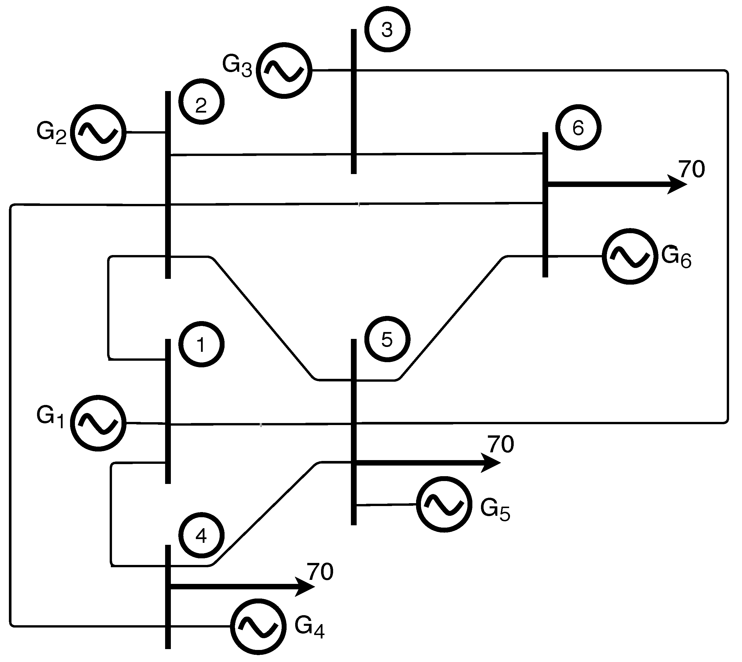
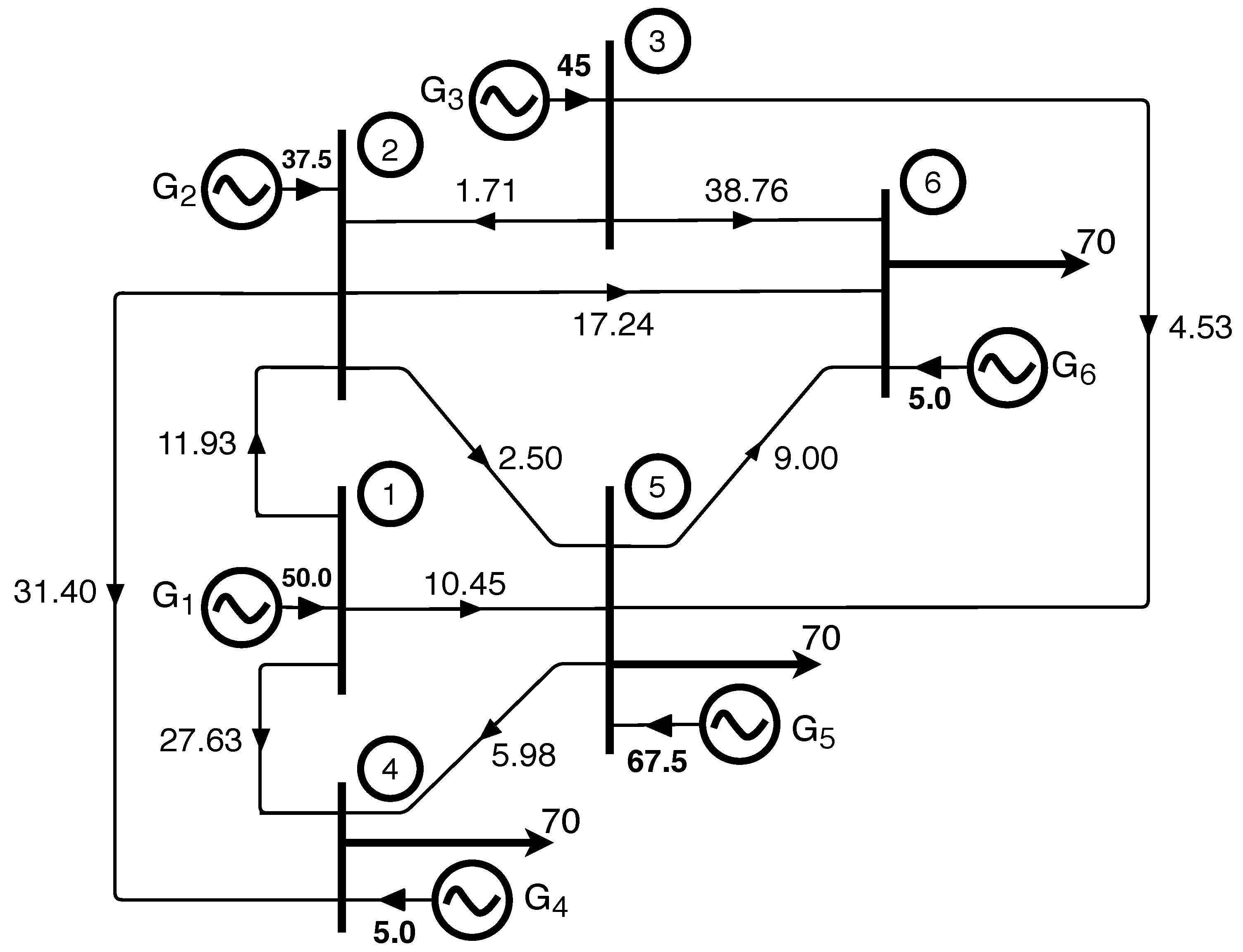
3.1. SCOPF Formulation Applied to an Example Power System (6-Bus)

The first security-constrained simulation takes into account the 6-bus power system presented by Wood and Wollenberg [8]. Transmission network data can be seen in [8] or in MatPower [22].

In comparison with the original generation system, three new power units are located at each load bus ($G_4$, $G_5$ and $G_6$). Figure 1 shows the electrical power system.

Technical data for the power generation system are given in

Table 1. Power generation technical parameters.

Power	A	B	C	${\mathit{P}}^{\mathit{min}}$	${\mathit{P}}^{\mathit{max}}$	${\mathit{R}}^{\mathit{up}}$	${\mathit{R}}^{\mathit{down}}$
Unit	($\$/{\mathbf{MW}}^2\mathbf{h}$)	($\$/\mathbf{MWh}$)	($/h)	(MW)	(MW)	(MW/min)	(MW/min)
$G_1$	0.00533	11.669	213.1	200	50	9.0	8.5
$G_2$	0.00889	10.333	200.0	150	37.5	12.0	12.0
$G_3$	0.00741	10.833	240.0	180	45	11.0	10.1
$G_4$	0.00301	14.198	40.0	70	5	2.5	5.0
$G_5$	0.00111	4.955	300.0	70	5	4.0	2.0
$G_6$	0.00876	18.003	10.0	70	5	3.5	5.0

. Besides, ramp-up and ramp-down characteristics are incorporated in the last two columns for each power unit.

Solving the classical OPF problem, the optimal cost is C_total = 3003.17 $/h. The power generation solution is P₁ = 50.0 MW, P₂ = 37.5 MW, P₃ = 45.0 MW, P₄ = 5.0 MW, P₅ = 67.5 MW and P₆ = 5.0 MW. Figure 2 shows the power flow solution. According to the power flow solution, there is no congestion in transmission elements. PyPower [23] is used to validate the solution and both solutions are the same.

To realize possible transmission effects, the maximum transmission limits are changed to 40 MW in lines 1–4, 2–4 and 3–6. With this new capacity, the OPF problem also obtains the same solution (operational cost, power unit generation and transmission power flows). This new transmission capacity is used to develop the N−1 power system security.

DC-Based and SF-Based SCOPF Formulations

In the first analysis, both classical (CL) and introduced (SF) problems are implemented to model the SCOPF. These formulations are subject to one pre- and eleven post-contingency constraints.

• Corrective SCOPF problem—for this analysis, power generation data are incorporated in the formulation assuming that the ISO has 10 min to eliminate overloading transmission effects and to recover the steady-state power system security. The main advantage of the corrective formulation is related to the operator clearly knows the post-contingency economic dispatch. This solution considers not only technical generation constraints but the variable fuel cost of each power unit. Indeed, the new power generation setting will achieve a safety and robust security-constrained N−1 solution no matter which transmission element failure.

Two cases are conducted to determine effects when ramps constraints are added in the SCOPF problem. These optimization problems have been solved using the SF-based formulation. Results are the following:

Case 1

Without ramp constraints—the operational cost is 3003.17 $/h for the pre-contingency condition and 3487.87 $/h for the post-contingency condition and the optimal total cost is C_total = 6491.04 $/h. Actually, the pre-contingency cost is the same than the traditional OPF problem (3003.17 $/h).

Case 2

Including ramp-up and -down constraints—the cost is 3146.35 $/h for the pre-contingency condition and 3487.87 $/h for the post-contingency condition and the total cost is C_total = 6634.22 $/h. For this case, the number of decision variables is 12 and the number of constraints is 280.

Table 2. Power generation solution for pre- and post-contingency states.

Power	Without-Ramps		With-Ramps
Unit	Pre-Contingency	Post-Contingency	Difference	Pre-Contingency	PosT-Contingency	Difference
#	Power, MW	Power, MW	MW	Power, MW	Power, MW	MW
P${}_1$	50.00	50.00	0	50.00	50.00	0
P${}_2$	37.50	37.50	0	60.86	37.50	+23.36
P${}_3$	45.00	45.00	0	45.00	45.00	0
P${}_4$	5.00	27.24	−22.24	5.00	27.24	−22.24
P${}_5$	67.50	24.14	+36.36	44.14	24.14	+20.00
P${}_6$	5.00	26.12	−21.12	5.00	26.12	−21.12

shows the results, operational cost and power dispatch for each SCOPF solution. Positive values imply that the power unit generation must decrease its dispatch. With this information, the ISO rapidly decides (10 or 20 min) which generator would economically change the power unit setting to optimally eliminate overloading conditions.

Because PyPower does not formulated the security-constrained analysis, it is not possible to contrast this power generation solution.

Because of ramp constraints, the ISO will be not able to achieve a safe post-contingency steady-state with the solution obtained in Case 1). Therefore, the system operator will need to decrease the load of the customers or/and turn-on fast reserve power units.

Notice that the ramp-down constraint of power unit 5 (44.14 − 24.14 = 20 MW) is active with a shadow price of 6.36 $/MWh. Therefore, the pre-contingency cost is higher (143.18 $/h) than the traditional OPF problem. Additionally, the power generation solution for the post-contingency condition is the same for both cases.

In comparison with the SF-based formulation, simulation results obtained by the CL-based formulation are the same. Therefore, both formulations achieve the same optimal solution; that is, these optimization problems are equivalent.

Incorporating the ramp constraints in the CL SCOPF problem, the number of decision variables is 205 and the number of constraints is 483. Comparing with the SF formulation, there is a very significant reduction of 94.1% and 42.0%, respectively.

Figure 3 displays the pre- and the post-contingency solutions when line 1–2 is outage. Both solutions could be compared to realize redispatch effects in the transmission network for generation two, four, five and six (grey color).

Using the post-contingency power generation solution (Table 2), eleven N−1 power flows are computed. For detailed information,

Table 3. Power flow solution for each N−1 transmission contingency.

Line	1–4 MW	1–5 MW	2–3 MW	2–4 MW	2–5 MW	2–6 MW	3–5 MW	3–6 MW	4–5 MW	5–6 MW
-	24.21	19.95	10.38	−1.41	7.99	8.53	8.46	10.70	10.31	10.11
$f_{1–4}$	-	30.05	21.94	36.14	21.24	21.39	21.37	22.03	21.13	21.86
$f_{1–5}$	25.79	-	17.68	15.26	20.78	20.08	20.17	17.26	18.56	18.03
$f_{2–3}$	−1.51	2.37	-	2.09	1.67	5.91	−6.15	−16.98	−0.39	−0.98
$f_{2–4}$	40.00	20.20	23.12	-	26.49	25.73	25.83	22.66	21.63	23.49
$f_{2–5}$	9.65	16.73	10.76	16.20	-	14.39	14.54	10.13	11.68	11.29
$f_{2–6}$	13.57	18.15	14.00	17.81	17.32	-	11.74	32.40	14.89	13.81
$f_{3–5}$	12.58	17.02	13.69	16.69	16.22	10.91	-	28.02	13.86	13.96
$f_{3–6}$	30.91	30.36	31.31	30.40	30.46	40.00	38.85	-	30.75	30.06
$f_{4–5}$	−2.76	7.49	2.29	−6.62	4.96	4.36	4.44	1.93	-	2.59
$f_{5–6}$	−0.60	−4.63	−1.43	−4.33	−3.90	3.87	−6.71	11.47	−1.76	-

shows the power flow solution for each outage.

Results showed there are two post-contingency congestions in the following lines: (a) transmission line 2–4 when line 1–4 is out; and (b) transmission line 3–6 when line 2–6 is out. We have highlighted these values with bold. Based on the OPF solution, shadow prices (Lagrangian multipliers) for each congestion are the following: (a) for line 2–4 is 28.60 $/MWh; and (b) for line 3–6 is 41.98 $/MWh. The OPF overcost and the bigger Lagrangian multipliers are produced by transmission congestion and ramp-down constraint of unit 5.

• Preventive SCOPF problem—the main advantage of this formulation is related to the operator does not need to modify the post-contingency power dispatch.

Using the SF-based formulation, the number of decision variables is 6 and the number of constraints is 280. The optimal cost obtained by Gurobi is C_total = 3487.87 $/h which was previously obtained. In the solution, there is no congestion in the pre-contingency condition. However, there is congestion in transmission line 2–4 (when line 1–4 is out) and line 3–6 (when line 2–6 is out).

Gurobi achieves the same solution solving the CL-based SCOPF formulation. Nevertheless, the number of decision variables is 199 and the number of constraints is 459.

To compare corrective and preventive SCOPF solutions, the power dispatch obtained in the pre-contingency condition must be compared for both solutions. The preventive overcost is 342.52 $/h (9.82%). Therefore, there is an important operational saving cost obtained by the corrective formulation.

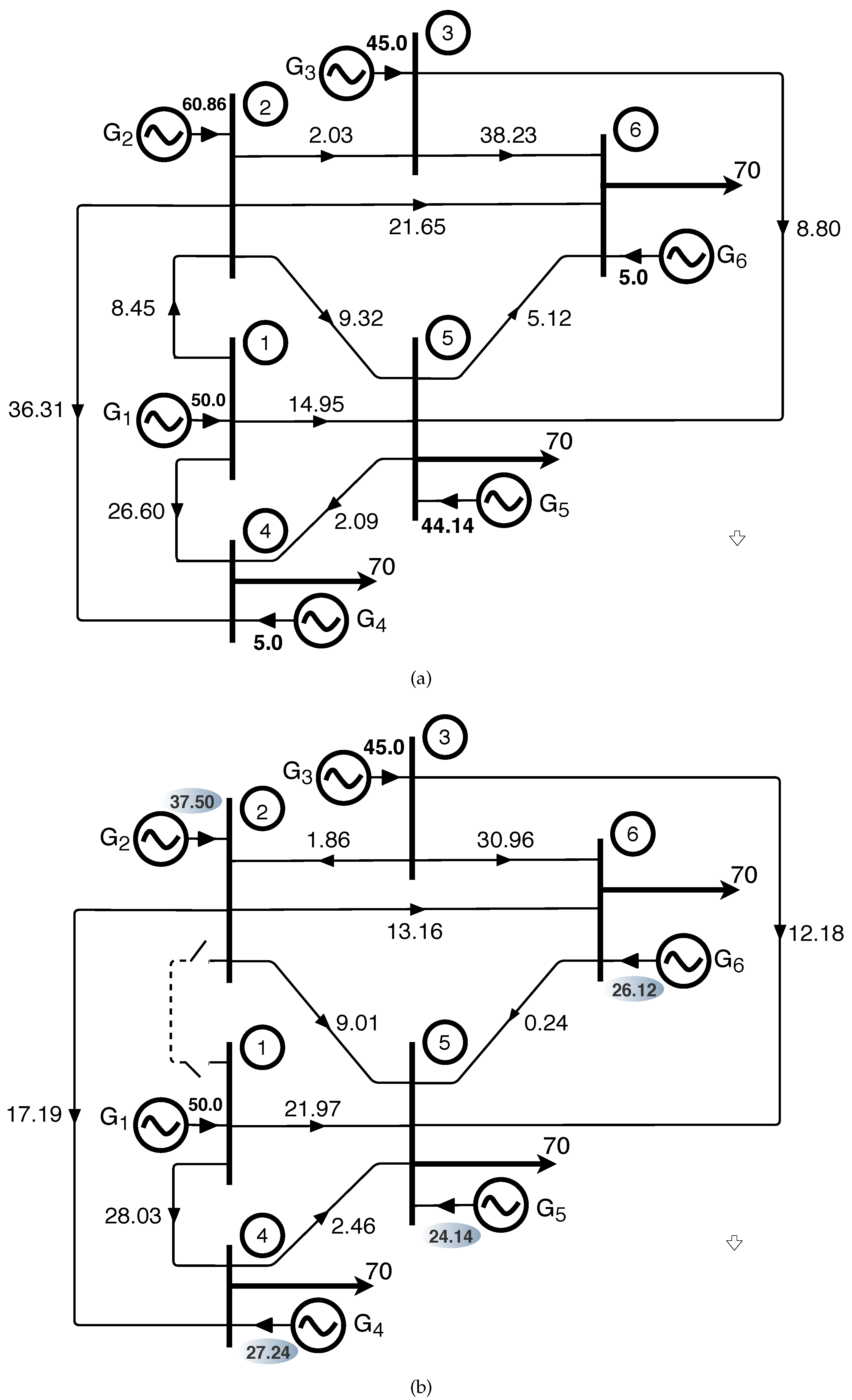
3.2. Corrective SCOPF Using a Ranking of Contingencies

In real power systems, all contingencies do not result in a post-contingency alert condition [8]. To figure out the SCOPF problem, several authors have used as security criterion the most severe contingency [6].

Regarding the N−1 power flow solution obtained previously by the initial OPF (3003.17 $/h), we solves eleven power flows for each N−1 post-contingency event. Simulations have shown there are five overloading states: (a) when line 1–4 is out, the power flow in line 2–4 is 131.32%; (b) when line 2–4 is out, the power flow in line 1–4 is 117.11%; (c) when line 2–6 is out, the power flow in line 3–6 is 124.41%; (d) when line 3–5 is out, the power flow in line 3–6 is 103.70%; and (e) when line 5–6 is out, the power flow in line 3–6 is 109.42%. Indeed, the ranking of overloading contingencies is the following: (1) line 1–4, (2) line 2–6, (3) line 2–4, (4) line 5–6 and (5) line 3–6.

The outage of these transmission elements produce a risky operational condition and probably technical problems to supply adequately the load of the customers. In the next analysis, each line of this ranking will be added in the SCOPF problem.

Table 4. Security-constrained operational cost considering the ranking of contingencies.

Optimal Solution	(i) N−1: line1–4 $/h	(ii) N−1: line2–6 $/h	(iii) N−1: line2–4 $/h	(iv) N−1: line5–6 $/h	(v) N−1: line1–4 and line2–6 $/h
n	12	12	12	12	12
$n_e$ + $n_i$	80	80	80	80	100
$Cos{t}_{pre}$	3003.17	3003.17	3003.17	3003.17	3146.36
$Cos{t}_{post}$	3178.12	3241.03	3122.32	3091.56	3487.87
$Cos{t}_{total}$	6181.29	6244.21	6125.49	6094.74	6634.22

displays the number of decision variables and constraints and the objective function solving the SCOPF problem.

• For the first case, the pre-contingency and the worst contingency (line 1–4) constraints are simultaneously incorporated in the SCOPF problem.
  Solving the SCOPF problem, the post-contingency power unit solution is used to validate electrical system security using eleven N−1 power flow problems. Simulation results show there are three overloading conditions: (a) when transmission line 2–6 is out, the power flow in line 3–6 is 51.18 MW; (b) when transmission line 3–5 is out, the power flow in line 3–6 is 42.74 MW; and (c) when transmission line 5–6 is out, the power flow in line 3–6 is 42.11 MW. Notice that the maximum power flow in line 3–6 is 40 MW. Therefore, a SCOPF problem based on the worst contingency does not guarantee a safe post-contingency operational point.
• In the second case, the SCOPF problem includes the outage of the transmission line 2–6.
  Reviewing the power flow solution, there are two overloading conditions: (a) when transmission line 1–4 is out, the power flow in line 2–4 is 54.34 MW; and (b) when transmission line 2–4 is out, the power flow in line 1–4 is 47.72 MW. Notice that the maximum power flow in line 1–4 and line 2–4 is 40 MW. Even though the operational cost is bigger than the previous case, this solution does not guarantee a safe power system as well. Additionally, this solution obtains the most overloading condition in line 2–4 (136%).
• In the third case, failure of transmission line 2–4 is added in the optimization problem.
  Simulating the N−1 post-contingency power flow method, the overloading conditions are the following: (a) when transmission line 1–4 is out, the power flow in line 2–4 is 43.97 MW; (b) when transmission line 2–6 is out, the power flow in line 3–6 is 50.73 MW; (c) when transmission line 3–6 is out, the power flow in line 2–6 is 41.62 MW; and (d) when transmission line 5–6 is out, the power flow in line 3–6 is 42.63 MW. Furthermore, this is an unacceptable post-contingency overloading condition.
• For the fourth case, transmission constraints for the outage of transmission line 5–6 is included in the N−1 optimization problem.
  Simulating the post-contingency power flow method, the overloading conditions are the following: (a) when transmission line 1–4 is out, the power flow in line 2–4 is 53.20 MW; (b) when transmission line 2–4 is out, the power flow in line 1–4 is 47.17 MW; (c) when transmission line 2–6 is out, the power flow in line 3–6 is 46.11 MW; and (d) when transmission line 3–5 is out, the power flow in line 3–6 is 40.16 MW.
• We do not show the last contingency because power flow results also display an overloading condition.

Finally, the post-contingency analysis including two N−1 candidate lines is developed. The SCOPF problem incorporates two major contingencies: line 1–4 and line 2–6. This framework adds in the optimization problem simultaneously one set of pre-contingency constraints and two sets of post-contingency constraints. For this optimization problem, the achieved solution is the optimal (the same solution considering the outage of all lines).

Table 4 also shows a reduction of 35.7% in constraints with respect to the original problem. In addition, both problems have the same number of decision variables.

As a result, the SCOPF problem should be modelled not only with the worst contingency but also with two or more contingencies to avoid risky operational conditions and technical problems to supply the load of the customers.

3.3. SCOPF Methodology Applied to Different-Scale Power Systems

We employ different electrical power test systems to determine the performance of both corrective and preventive SCOPF formulations using the SF-based as well as the CL-based frameworks: 14-bus system (five generators and twenty transmission lines); 57-bus system (seven generators and eighty transmission lines); 118-bus system (fifty-four generators and one hundred eighty-six transmission lines); and 300-bus system (sixty-nine generators and four hundred eleven transmission lines). PyPower shows technical information.

3.3.1. Corrective and Preventive Formulations

Because PyPower does not include ramp generation constraints, we have selected these limits using random numbers provided by a normal distribution function with a mean of 7 MW/min and a variance of 1.

Table 5. Simulation results using different power systems.

Formulation	Corrective				Preventive
System	$\mathit{OF}$, $/h	n	${\mathit{n}}_{\mathit{i}}+{\mathit{n}}_{\mathit{e}}$	$\mathit{ts}$, s	$\mathit{OF}$, $/h	n	n${}_{\mathit{i}}$ + n${}_{\mathit{e}}$	$\mathit{ts}$, s
14-bus (CL)	15,285.19	704	1545	0.0040	7642.59	699	1525	0.0036
14-bus (SF)	15,285.19	10	832	0.0004	7642.59	5	811	0.0009
57-bus (CL)	82,013.47	10,895	23,645	0.0821	41,006.74	7760	16,832	0.0414
57-bus (SF)	82,013.47	14	6366	0.0048	41,006.74	7	9023	0.0049
118-bus (CL)	260,788.55	55,558	123,669	0.9203	130,394.28	55,807	124,127	0.8459
118-bus (SF)	260,788.55	108	62,312	0.3057	130,394.28	54	62,095	0.3106
300-bus (CL)	1,422,058.21	71,849	155,048	0.8777	711,029.11	71,780	154,772	0.9468
300-bus (SF)	1,422,058.21	138	21,110	0.1350	711,029.11	69	20,833	0.1349

shows simulation results for both corrective and preventive analyses applying the CL and the SF formulations. For each SC problem, we have included the objective function ($OF$), the number of decision variables (n), constraints ($n_i+n_e$) and the average simulation time considering 200 trials.

For both 14-bus and 57-bus power systems, the security-constrained problem models the outage of all transmission lines.

Considering the higher simulation time obtained by a complete N−1 analysis, a reduced number of contingencies should be used to solve the security problem applied to large-scale power systems. In the 118-bus and the 300-bus systems, we have modelled the N−1 analysis using 176 transmission and 100 transmission candidate lines, respectively. This assumption is accomplished not only by the bigger number of variables and constraints but also by the higher simulation time.

For all power systems, there is an important improvement in the simulation time. Comparing both classical and SF-based formulations applied to the 300-bus system, SF-based formulation achieves the best performance with an efficiency of 6.97 times using the corrective formulation and 7.02 times using the preventive formulation.

Simulation results have shown the corrective formulation obtains the lower $OF$ in comparison with the preventive formulation.

Notice that the reactance bus matrix needs an inverse method.Therefore, the main disadvantage of the proposed methodology is the time computing to obtain the SF matrix. However, the security-constrained analysis could be carried out using an off-line SF matrix; that is, the SF matrix does not need to compute each N−1 time. Therefore, an external file could be used to save these matrixes improving the formulation time.

The LODF matrix could be computed using basic mathematical operations—Equation (37). Therefore, the computation time is not significant.

3.3.2. Another Classical DC-Based Preventive Formulation Applied to the 300-Bus Power System

In the following analysis, we use a different preventive SCOPF formulation. For this approach, power flow variables are eliminated from the optimization problem using two admittance bus matrixes ($Bbu{s}^{pre}$ and $Bbu{s}^{post}$). Consequently, there are only two sets of nodal balance constraints for the pre- and post-contingency analyses. Besides, the primitive-admittance incidence matrix for the pre-contingency $B{f}^{pre}$ and the post-contingency $B{f}^{post}$ conditions is substitute to determine transmission power flows.

Simulating 200 trials, the average simulation time is 0.7648 s for the preventive SCOPF problem which is 19.22% lower than the original CL-based formulation. For this mathematical problem, the number of decision variables is 30,369 and the number of constraints is 113,361. Therefore, the new classical formulation causes a reduction of 57.69% in the number of decision variables and a reduction of 26.76% in the number of equality and inequality constraints. Although there is an improvement in the simulation performance, this time is still higher (5.67 times) than the SF-based formulation.

Based on simulations, the introduced SF-based formulation achieves the best simulation time to carry out the corrective formulation and the preventive formulation applied to the SCOPF problem. This improvement is obtained by the lower number of decision variables as well as by the lower number of equality and inequality constraints. Therefore, this framework could be recommended to solve very large-scale power systems.

3.4. Corrective and Preventive SCOPF Methodology Applied to the Chilean Electrical Power System

The Chilean Interconnected Power System (in Spanish, SEN: Sistema Eléctrico Nacional) is used to validate both SCOPF formulations. Concerning the lower simulation time accomplished previously, the SF-based methodology is only applied to the SCOPF problem.

In January, 2019, the SEN generation capacity was 21,189.95 MW. In 2019, the peak load was 9382.7 MW. Review the Regulatory Company webpage (CNE: www.cne.cl) or the ISO webpage (CEN: www.coordinador.cl) to obtain more technical information.

The electrical power system contains one hundred fifty-nine buses, three hundred twenty-one transmission lines from 110 to 500 kV and two hundred sixty-seven generation power units (thermal, hydro and renewable energy). The webpage link https://infotecnica.coordinador.cl displays detailed technical and economic information about the Chilean study case.

For the power generation system, there are one hundred three renewable power units. For hydro, wind and solar, a capacity factor of 20%, 20% and 30% are selected, respectively. For thermal units, random numbers model ramp generation constraints for each power unit. Additionally, one hundred transmission lines are randomly selected to formulate the N−1 security-constrained analysis.

• Corrective SCOPF problem—this optimization problem has 534 decision variables and 22,082 constraints. The cost is 326,948.31 $/h for the pre-contingency condition and 327,087.37 $/h for the post-contingency condition. The simulation time is 1.0218 s using 100 trials.
  There is congestion in Cardones-Maintencillo 220 kV in the pre-contingency solution. On the contrary, there is post-contingency congestion in the following transmission elements—(1) Andes-Nueva Zaldivar 220 kV when Antucoya-Antucoya aux. 220 kV is out; (2) Antofagasta-Desalant 110 kV when Atacama-Esmeralda 220 kV is out; (3) Capricornio-Mantos Blancos 220 kV when CD Arica-Tap Quiani 66 kV is out; (4) Carrera Pinto-Carrera Pinto aux. 220 kV when Charrúa-Lagunillas 220 kV is out; and (5) CD Arica-Arica 66 kV when Charrúa-Mulchen 220 kV is out.
• Preventive SCOPF problem—this optimization problem has 267 decision variables and 21,013 constraints. The optimal cost is 329,981.43 $/h and the simulation time is 0.6085 s. For the pre-contingency condition, there is congestion in the same line (Cardones-Maintencillo 220 kV). Furthermore, there are seven lines with congestion in the post-contingency condition: (1) Andes-Nueva Zaldivar 220 kV; (2) Antofagasta-Desalant 110 kV; (3) Capricornio-Mantos Blancos 220 kV; (4) Carrera Pinto-Carrera Pinto aux. 220 kV; (5) CD Arica-Arica 66 kV; (6) Charrúa-Hualpen 220 kV (when Colbún-Ancoa 220 kV is out); and (7) Crucero-Nueva Crucero/Encuentro 220 kV (when Don Goyo-Don Goyo aux. 220 kV is out).

Even though the security cost is similar, the OPF formulation only considers one load time-period. Moreover, the unit commitment solution obtained by the ISO should be incorporated in the OPF problem to realize real saving costs.

4. Conclusions

This study analyzed two very effective methodologies to solve both corrective and preventive security-constrained DC optimal power flow problems using shift-factors. We used these factors to formulate pre- and post-contingency steady-state conditions. The optimal solution was found with lower number of decision variables and constraints in comparison with the traditional (CL) SCOPF formulation. To validate simulation time, a lot of analyses were conducted to determine which methodology obtained the best performance solving the SCOPF problem with different-scale test power systems.

The research group believes that the introduced security-constrained methodology could be applied to formulate deterministic and stochastic power system issues where the transmission topology does not change. For instance, unit commitment, generation planning, among other power system problems.

References

- Carpentier, J. Contribution a L’etude du Dispatching Economique. Bull. Soc. Fr. Electr. 1962, 8, 431–447. [Google Scholar]
- Bai, W.; Lee, D.; Lee, K.-Y. Stochastic dynamic AC optimal power flow based on a multivariate short-term wind power scenario forecasting model. Energies 2017, 10, 2138. [Google Scholar] [CrossRef]
- Momoh, J.; Adapa, R.; El-Hawary, M. A review of selected optimal power flow literature to 1993. IEEE Trans. Power Syst. 1993, 14, 96–104. [Google Scholar] [CrossRef]
- Pizano, A.; Fuerte, C.R.; Ruiz, D. A new practical approach to transient stability constrained optimal power flow. IEEE Trans. Power Syst. 2011, 26, 1686–1696. [Google Scholar] [CrossRef]
- Mohagheghi, E.; Alramlawi, M.; Gabash, A.; Li, P. Incorporating charging/discharging strategy of electric vehicles into security-constrained optimal power flow to support high renewable penetration. Energies 2017, 10, 729. [Google Scholar]
- Hinojosa, V.; Gonzalez-Longatt, F. Preventive security-constrained DCOPF formulation using power transmission distribution factors and line outage distribution factors. Energies 2018, 11, 1497. [Google Scholar] [CrossRef]
- Gutierrez-Alcaraz, G.; Hinojosa, V. Using generalized generation distribution factors in a MILP model to solve the transmission-constrained unit commitment problem. Energies 2018, 11, 2232. [Google Scholar] [CrossRef]
- Wood, A.J.; Wollenberg, B.F. Power Generation, Operation and Control; John Wiley & Sons: Hoboken, NJ, USA, 1996. [Google Scholar]
- Gonzalez-Longatt, F.; Rueda, J.L. Power Factory Applications for Power System Analysis; Springer: Berlin, Germany, 2014. [Google Scholar]
- Hinojosa, V.H.; Velásquez, J. Improving the mathematical formulation of security-constrained generation capacity expansion planning using power transmission distribution factors and line outage distribution factors. Electr. Power Syst. Res. 2016, 140, 391–400. [Google Scholar] [CrossRef]
- Alsac, O.; Stott, B. Optimal Load Flow with Steady-State Security. IEEE Trans. Power Appar. Syst. 1974, 93, 745–751. [Google Scholar] [CrossRef]
- Capitanescu, F.; Martinez-Ramos, J.L.; Panciatici, P.; Kirschen, D.; Marano-Marcolini, A.; Platbrood, P.; Wehenkel, L. State-of-the-art, challenges, and future trends in security constrained optimal power flow. Electr. Power Syst. Res. 2012, 81, 275–285. [Google Scholar] [CrossRef]
- Sass, F.; Sennewald, T.; Marten, A.; Westermann, D. Mixed AC high-voltage direct current benchmark test system for security constrained optimal power flow calculation. IET Gener. Transm. Distrib. 2017, 11, 447–455. [Google Scholar] [CrossRef]
- Martínez-Lacañina, P.; Martínez-Ramos, J.; de la Villa-Jaén, A. DC corrective optimal power flow base on generator and branch outages modelled as fictitious nodal injections. IET Gener. Transm. Distrib. 2014, 8, 401–409. [Google Scholar]
- Monticelli, A.; Pereira, M.V.F.; Granville, S. Security-constrained optimal power flow with post-contingency corrective rescheduling. IEEE Trans. Power Syst. 1987, 2, 175–180. [Google Scholar] [CrossRef]
- Dzung, P.; Kalagnanam, J. Some efficient optimization methods for solving the security-constrained optimal power flow problem. IEEE Trans. Power Syst. 2014, 29, 863–872. [Google Scholar]
- Phan, D.; Sun, X. Minimal impact corrective actions in security-constrained optimal power flow via sparsity regularization. IEEE Trans. Power Syst. 2015, 30, 1947–1956. [Google Scholar] [CrossRef]
- An, K.; Song, K.; Hur, K. A survey of real-time optimal power flow. Energies 2018, 11, 3142. [Google Scholar]
- Wu, X.; Zhou, Z.; Liu, G.; Qi, W.; Xie, Z. Preventive security-constrained optimal power flow considering UPFC control modes. Energies 2017, 10, 1199. [Google Scholar] [CrossRef]
- Python. Available online: http://www.python.org (accessed on 1 December 2019).
- Gurobi Optimization. Available online: http://www.gurobi.com (accessed on 1 December 2019).
- Matpower. Available online: http://www.pserc.cornell.edu/matpower (accessed on 1 December 2019).
- Pypower. Available online: https://pypi.org/project/PYPOWER/ (accessed on 13 December 2019).