Validation of Actuator Line and Vortex Models Using Normal Forces Measurements of a Straight-Bladed Vertical Axis Wind Turbine


Abstract
1. Introduction
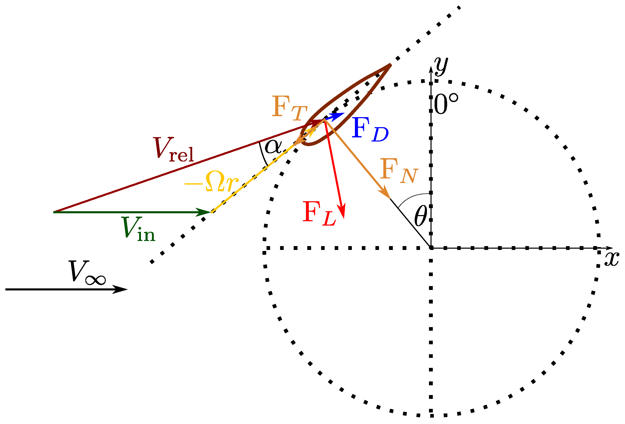
2. Theory
2.1. The Actuator Line Model
2.1.1. The Large Eddy Simulation Framework
2.1.2. The Smagorinsky Model
2.2. The Vortex Model
- Calculate the circulation from potential flow solution using the panel method and evaluate the relative flow velocity at the quarter chord position
- Convert the circulation to an angle of attack using the calibrated lookup table
- Calculate the circulation from Kutta Joukowski’s lift formula
- Determine the released circulation from the change in circulation add add these vortices to the flow
- Calculate the flow velocity at each vortex point using Biot-Savart’s law and propagate all vortices with the flow speed
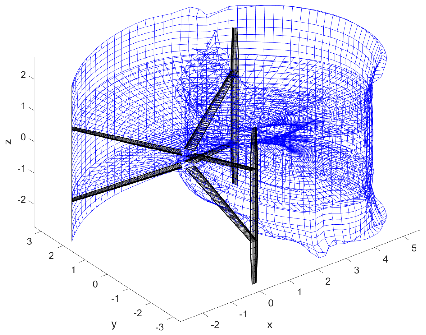
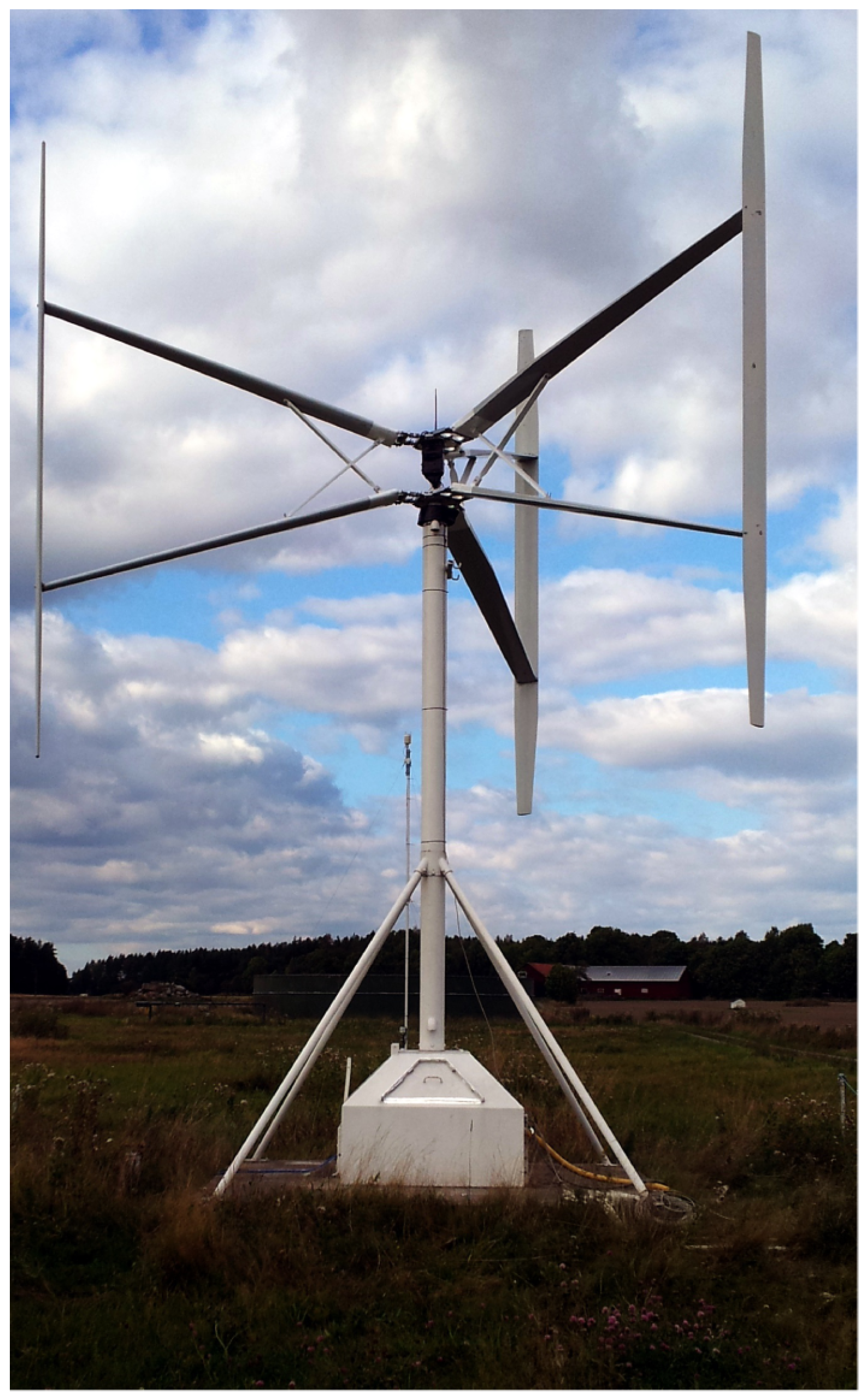
3. Simulation Parameters: Validation Case
4. Results and Discussion
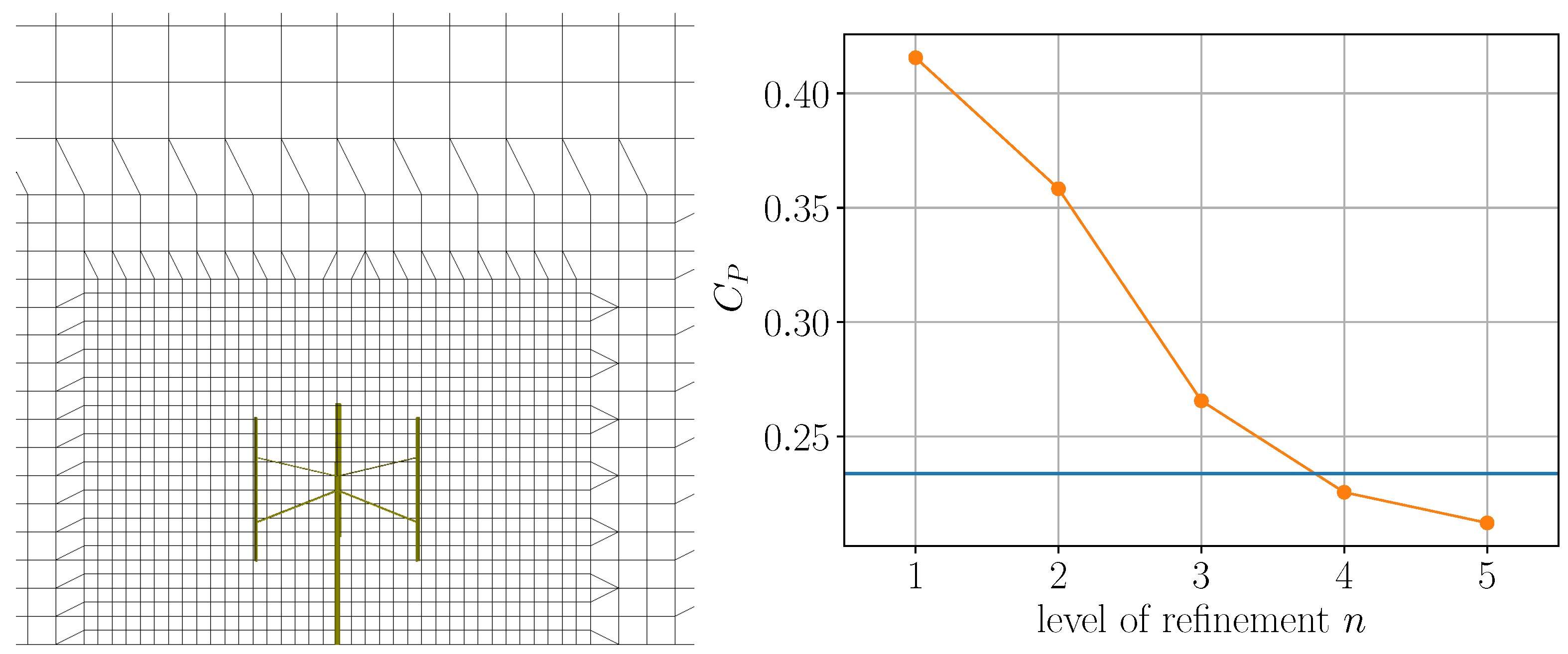
4.1. Spatial Sensitivity of the ALM
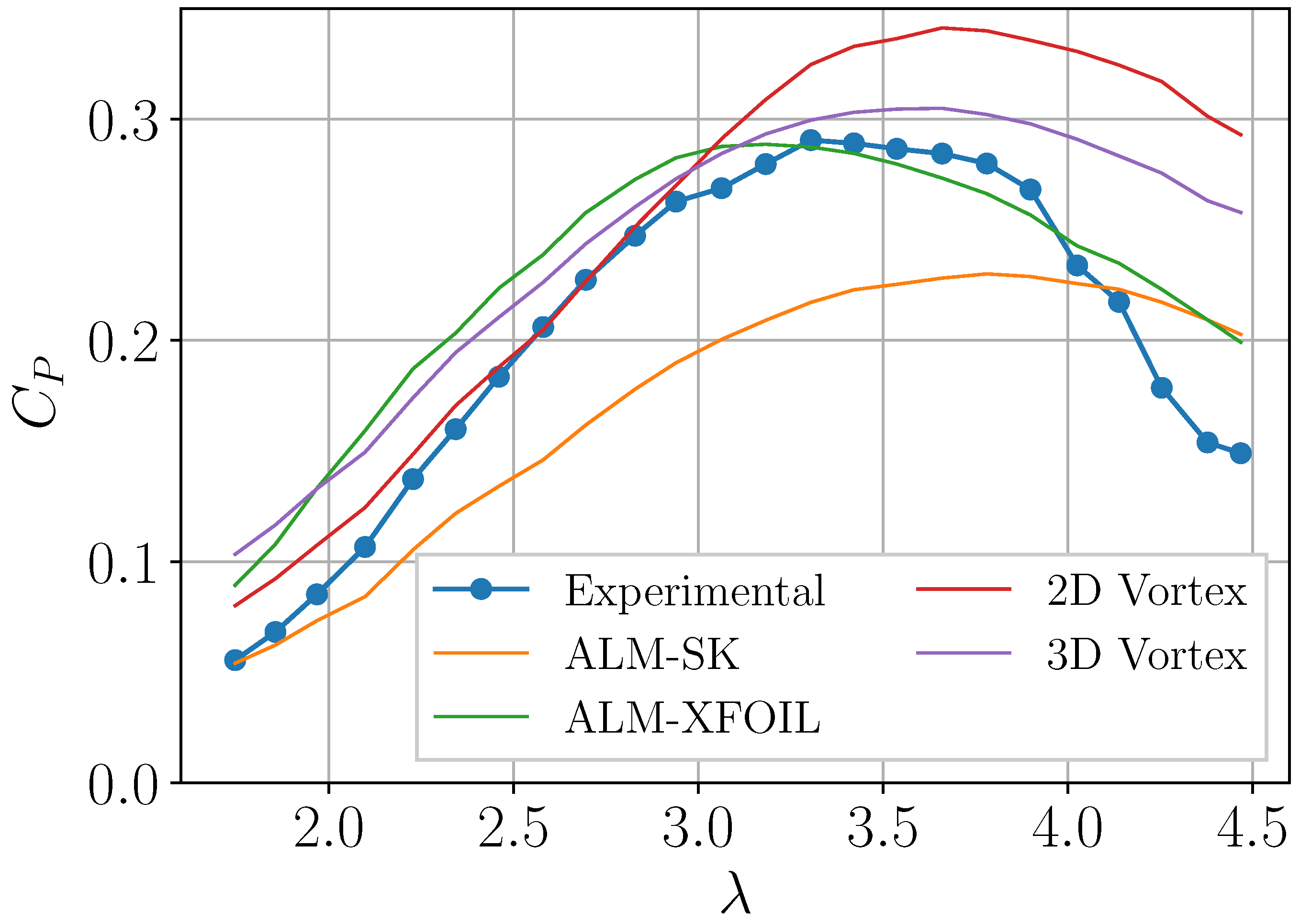
4.2. Power Coefficient Curve
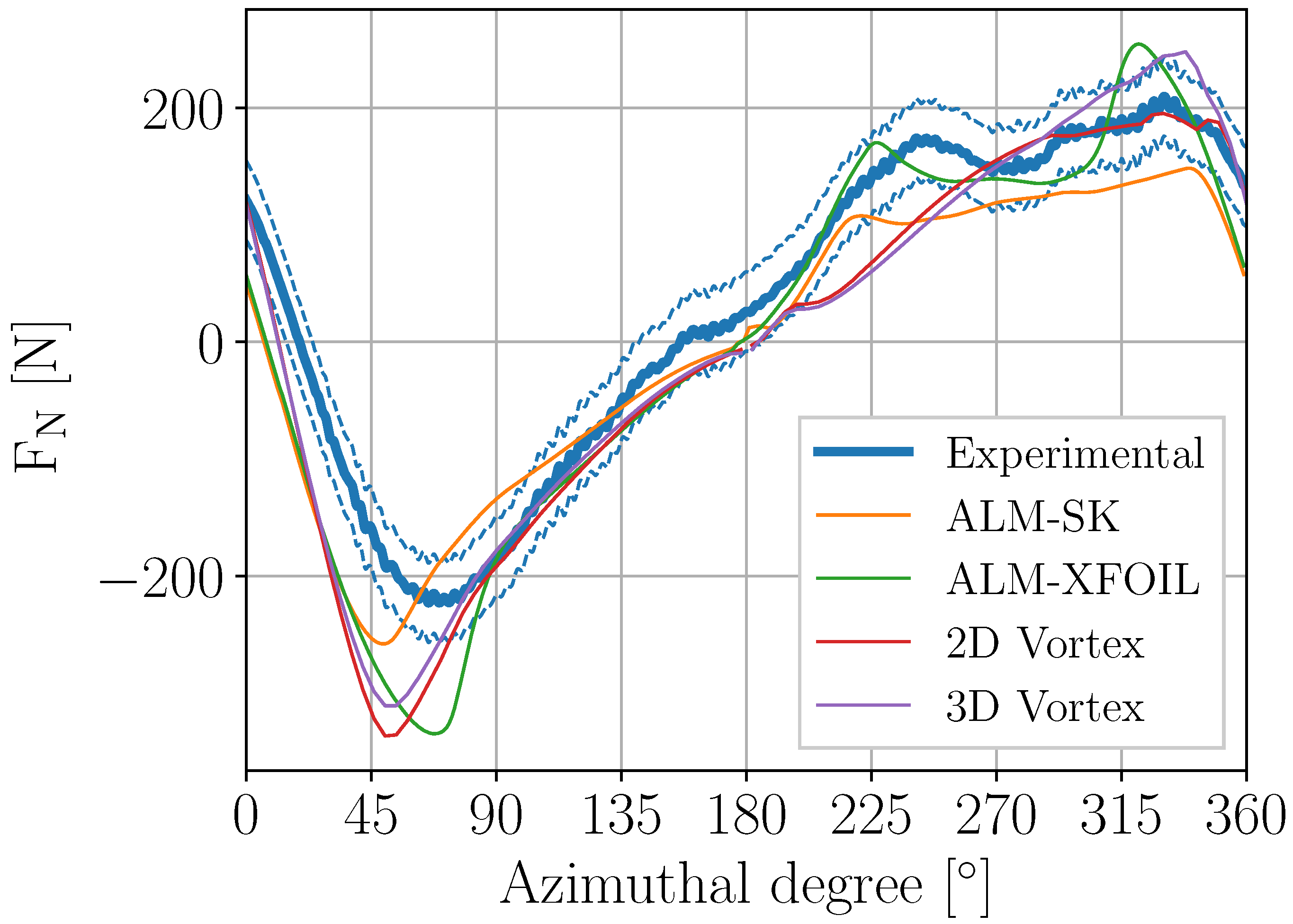
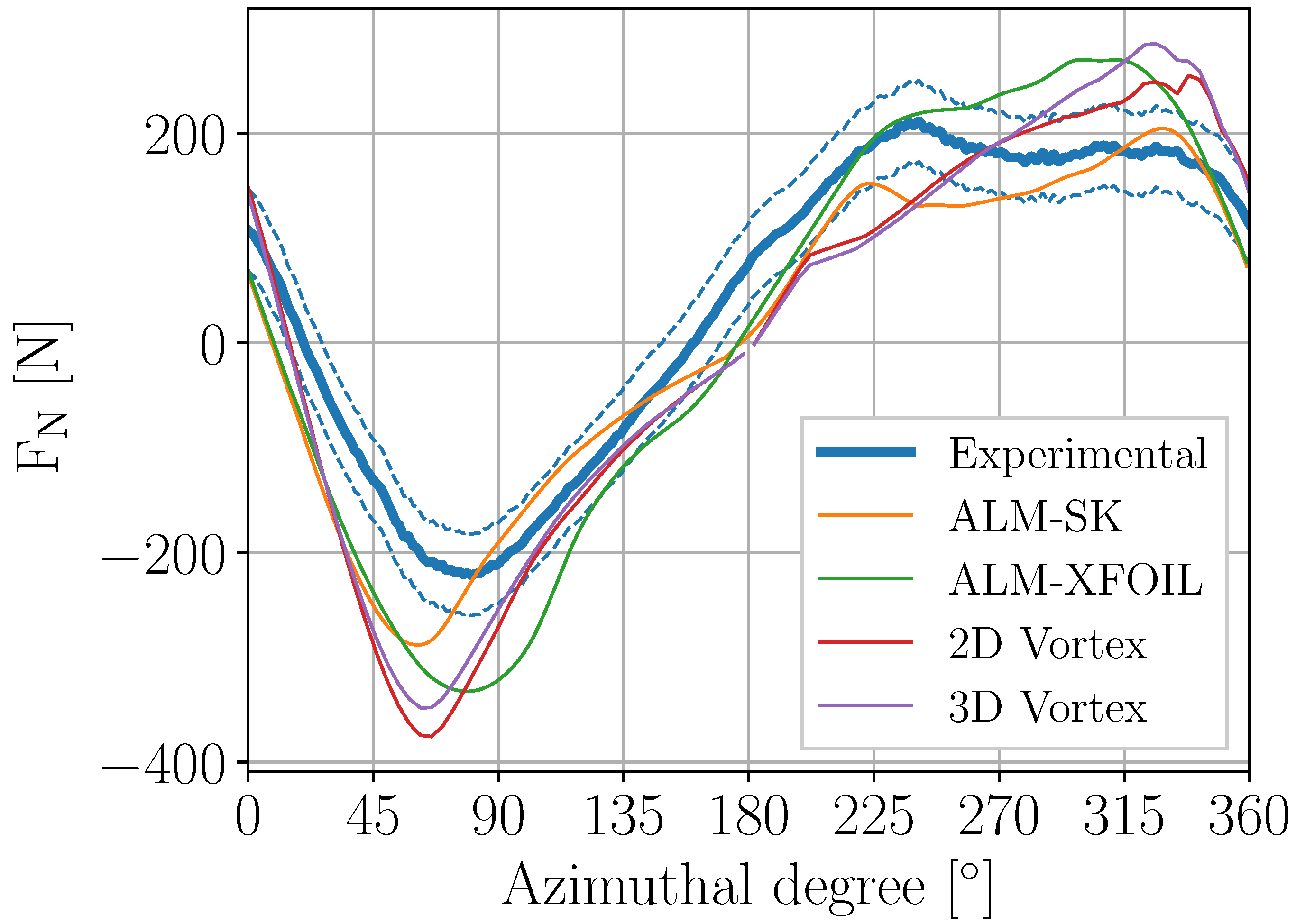
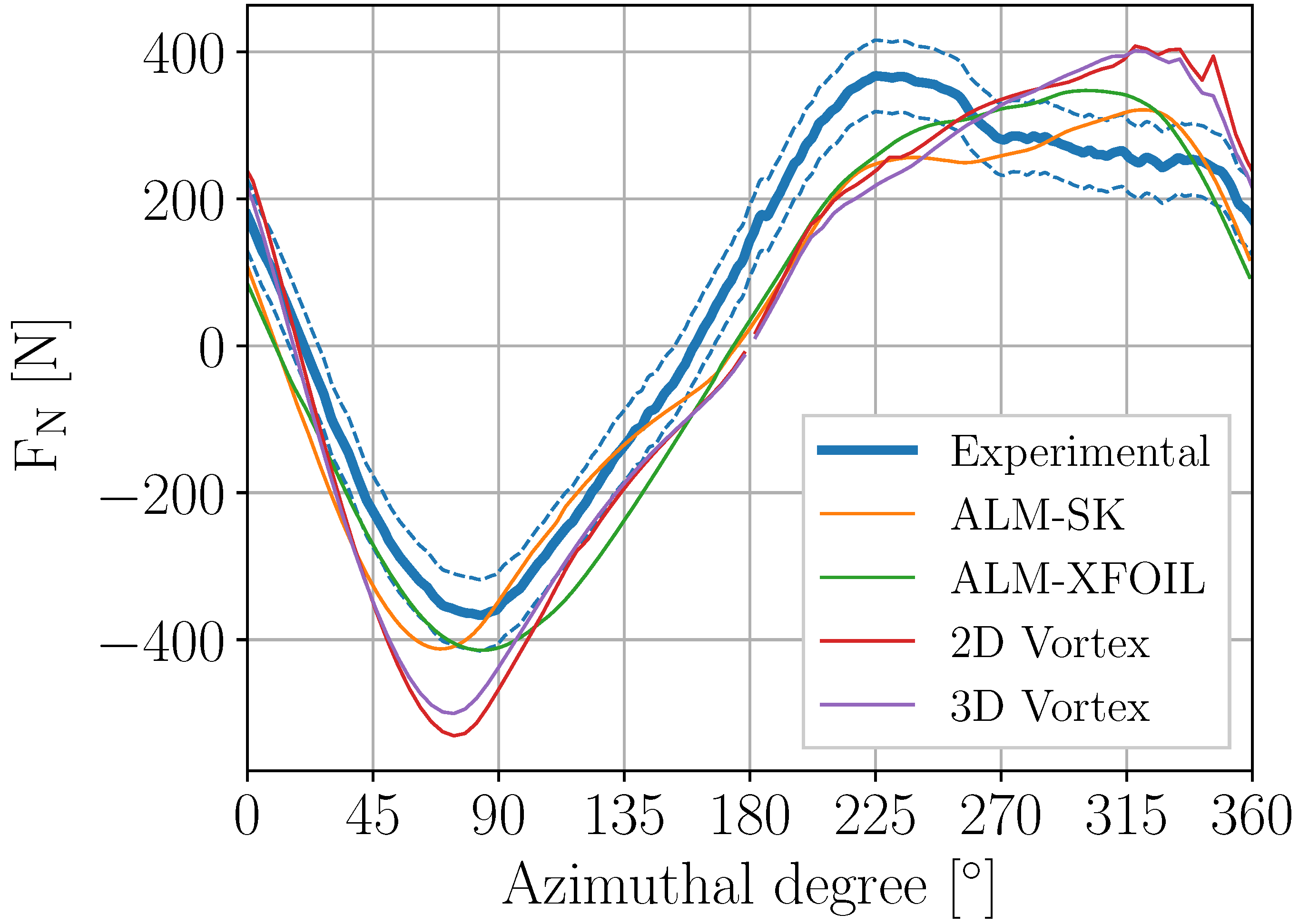
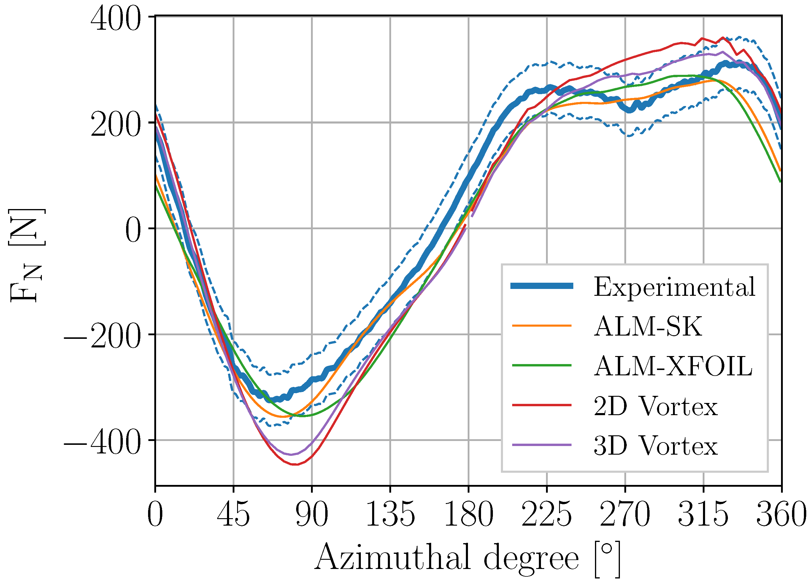
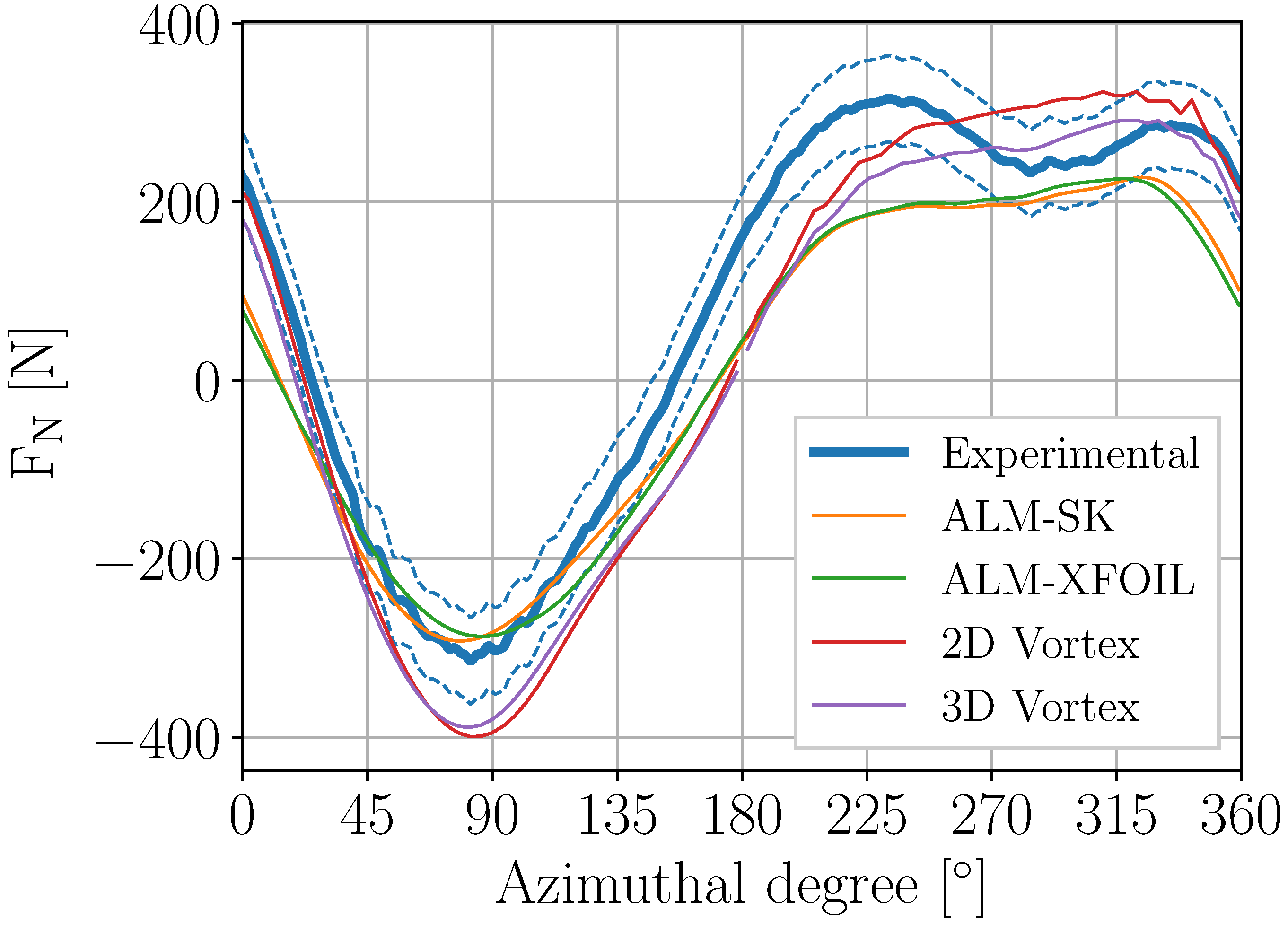
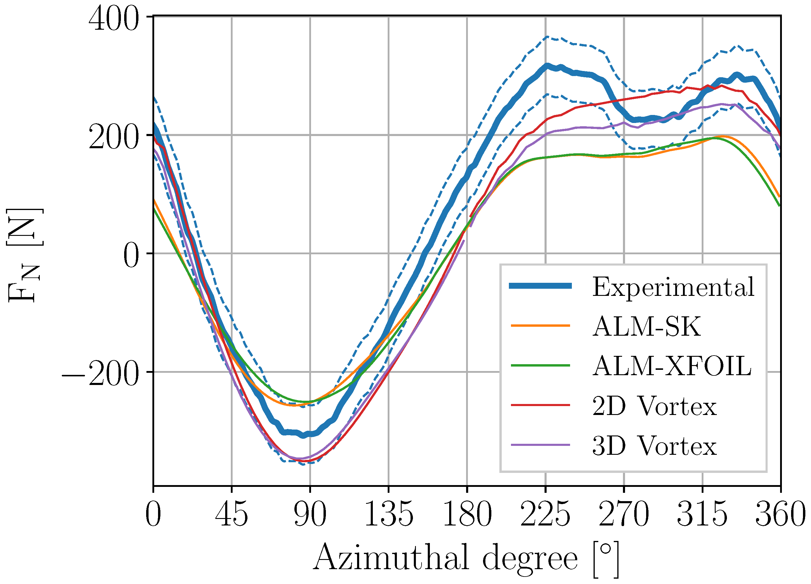
4.3. Normal Forces
4.4. General Discussion
5. Conclusions
Author Contributions
Funding
Acknowledgments
Conflicts of Interest
References
- Vita, L.; Paulsen, U.S.; Pedersen, T.F.; Madsen, H.A.; Rasmussen, F. Deep wind: A novel floating wind turbine concept. Wind. Int. 2010, 6, 29–31. [Google Scholar]
- Sandia National Laboratories. Offshore uSe of Vertical-Axis Wind Turbines Gets Closer Look. Available online: https://share-ng.sandia.gov/news/resources/news_releases/vawts/#.WKB9WHUrKp0 (accessed on 16 January 2018).
- Dodd, J. First 2MW Vertiwind Vertical-Axis Prototype Built. Available online: http://www.windpowermonthly.com/article/1305428/first-2mw-vertiwind-vertical-axis-prototype-built (accessed on 16 January 2018).
- Musgrove, P. Wind energy conversion: Recent progress and future prospects. Solar Wind Technol. 1987, 4, 37–49. [Google Scholar] [CrossRef]
- Borg, M.; Collu, M.; Brennan, F. Offshore floating vertical axis wind turbines: Advantages, disadvantages, and dynamics modelling state of the art. In Proceedings of the International Conference on Marine & Offshore Renewable Energy (MORE 2012), London, UK, 26–27 September 2012. [Google Scholar]
- Peace, S. Another approach to wind: Vertical-axis turbines may avoid the limitations of today’s standard propeller-like machines. Mech. Eng. 2004, 126, 28–32. [Google Scholar] [CrossRef]
- Ribrant, J.; Bertling, L. Survey of failures in wind power systems with focus on Swedish wind power plants during 1997–2005. In Proceedings of the Power Engineering Society General Meeting, Tampa, FL, USA, 24–28 June 2007; pp. 1–8. [Google Scholar]
- Tavner, P.; Xiang, J.; Spinato, F. Reliability analysis for wind turbines. Wind Energy 2007, 10, 1–18. [Google Scholar] [CrossRef]
- Arabian-Hoseynabadi, H.; Oraee, H.; Tavner, P. Failure modes and effects analysis (FMEA) for wind turbines. Int. J. Electr. Power Energy Syst. 2010, 32, 817–824. [Google Scholar] [CrossRef]
- Eriksson, S.; Solum, A.; Leijon, M.; Bernhoff, H. Simulations and experiments on a 12kW direct driven PM synchronous generator for wind power. Renew. Energy 2008, 33, 674–681. [Google Scholar] [CrossRef]
- Sutherland, H.; Berg, D.; Ashwill, T. A Retrospective of VAWT Technology; Sandia Report No. SAND2012-0304; Sandia National Laboratories: Albuquerque, NM, USA, 2012.
- Bachant, P.; Wosnik, M. Characterising the near-wake of a cross-flow turbine. J. Turbul. 2015, 16, 392–410. [Google Scholar] [CrossRef]
- Johnston, S.J. Proceedings of the Vertical Axis Wind Turbine (VAWT) Design Technology Seminar for Industry. Available online: http://www.osti.gov/scitech/servlets/purl/6725534/ (accessed on 1 January 2019).
- Atkins, R.E. Measurements of Surface Pressures on an Operating Vertical-Axis Wind Turbine; Sandia National Laboratories: Livermore, CA, USA, 1989.
- Oler, J.; Strickland, J.H.; Im, B.; Graham, G. Dynamic-Stall Regulation of the Darrieus Turbine; Tech. Rep.; Department of Mechanical Engineering, Texas Tech University: Lubbock, TX, USA, 1983. [Google Scholar]
- Strickland, J.H.; Webster, B.; Nguyen, T. A vortex model of the darrieus turbine: An analytical and experimental study. J. Fluids Eng. 1979, 101, 500–505. [Google Scholar] [CrossRef]
- Ashuri, T.; Bussel, G.; Mieras, S. Development and validation of a computational model for design analysis of a novel marine turbine. Wind Energy 2013, 16, 77–90. [Google Scholar] [CrossRef]
- Castelein, D.; Ragni, D.; Tescione, G.; Ferreira, C.S.; Gaunaa, M. Creating a benchmark of vertical axis wind turbines in dynamic stall for validating numerical models. In Proceedings of the 33rd Wind Energy Symposium 2015, American Institute of Aeronautics and Astronautics, 33rd AIAA/ASME Wind Energy Symposium, Kissimmee, FL, USA, 5–9 January 2015. [Google Scholar]
- Kjellin, J.; Bülow, F.; Eriksson, S.; Deglaire, P.; Leijon, M.; Bernhoff, H. Power coefficient measurement on a 12 kW straight bladed vertical axis wind turbine. Renew. Energy 2011, 36, 3050–3053. [Google Scholar] [CrossRef]
- Dyachuk, E.; Rossander, M.; Goude, A.; Bernhoff, H. Measurements of the aerodynamic normal forces on a 12-kW straight-bladed vertical axis wind turbine. Energies 2015, 8, 8482–8496. [Google Scholar] [CrossRef]
- Rossander, M.; Dyachuk, E.; Apelfröjd, S.; Trolin, K.; Goude, A.; Bernhoff, H.; Eriksson, S. Evaluation of a blade force measurement system for a vertical axis wind turbine using load cells. Energies 2015, 8, 5973–5996. [Google Scholar] [CrossRef]
- Mendoza, V.; Goude, A. Improving farm efficiency of interacting vertical-axis wind turbines through wake deflection using pitched struts. Wind Energy 2019, 22, 538–546. [Google Scholar] [CrossRef]
- Mendoza, V.; Chaudhari, A.; Goude, A. Performance and wake comparison of horizontal and vertical axis wind turbines under varying surface roughness conditions. Wind Energy 2019, 22, 458–472. [Google Scholar] [CrossRef]
- Mendoza, V.; Bachant, P.; Ferreira, C.; Goude, A. Near-wake flow simulation of a vertical axis turbine using an actuator line model. Wind Energy 2019, 22, 171–188. [Google Scholar] [CrossRef]
- Mendoza, V. Aerodynamic Studies of Vertical Axis Wind Turbines Using the Actuator Line Model. Ph.D. Thesis, Acta Universitatis Upsaliensis, Uppsala, Sweden, 2018. [Google Scholar]
- Bachant, P.; Wosnik, M. Simulating wind and marine hydrokinetic turbines with actuator lines in rans and les. In Proceedings of the APS Meeting Abstracts, San Antonio, TX, USA, 2–6 March 2015. [Google Scholar]
- Bachant, P.; Goude, A.; Wosnik, M. Actuator line modeling of vertical-axis turbines. arXiv 2016, arXiv:1605.01449. [Google Scholar]
- Bachant, P.; Goude, A.; Wosnik, M. Turbinesfoam: v0.0.7. Available online: https://zenodo.org/record/49422#.XjOHMWYRWHs (accessed on 16 April 2016).
- Mendoza, V.; Bachant, P.; Wosnik, M.; Goude, A. Validation of an actuator line model coupled to a dynamic stall model for pitching motions characteristic to vertical axis turbines. J. Phys. 2016, 753, 022043. [Google Scholar] [CrossRef]
- Mendoza, V.; Goude, A. Wake flow simulation of a vertical axis wind turbine under the influence of wind shear. J. Phys. 2017, 854, 012031. [Google Scholar] [CrossRef]
- Sørensen, J.N.; Shen, W.Z. Computation of wind turbine wakes using combined navier-stokes/actuator-line methodology. In Proceedings of the European Wind Energy Conference EWEC 99, Nice, France, 1–5 March 1999. [Google Scholar]
- Leishman, J.; Beddoes, T. A generalised model for airfoil unsteady aerodynamic behaviour and dynamic stall using the indicial method. In Proceedings of the 42nd Annual forum of the American Helicopter Society, Washington, DC, USA, 7–10 July 1986; pp. 243–265. [Google Scholar]
- Sheng, W.; Galbraith, R.; Coton, F. A modified dynamic stall model for low mach numbers. J. Solar Energy Eng. 2008, 130, 031013. [Google Scholar] [CrossRef]
- Dyachuk, E. Aerodynamics of Vertical Axis Wind Turbines: Development of Simulation Tools and Experiments. Ph.D. Thesis, Acta Universitatis Upsaliensis, Uppsala, Sweden, 2015. [Google Scholar]
- Smagorinsky, J. General circulation experiments with the primitive equations: I. the basic experiment. Mon. Weather Rev. 1963, 91, 99–164. [Google Scholar] [CrossRef]
- Yoshizawa, A. Subgrid-scale modeling suggested by a two-scale dia. In Computational Wind Engineering 1; Elsevier: Amsterdam, The Netherlands, 1993; pp. 69–76. [Google Scholar]
- Dyachuk, E.; Goude, A. Numerical validation of a vortex model against experimentaldata on a straight-bladed vertical axis wind turbine. Energies 2015, 8, 11800–11820. [Google Scholar] [CrossRef]
- Dyachuk, E.; Goude, A.; Berhnoff, H. Simulating Pitching Blade With Free Vortex Model Coupled with Dynamic Stall Model for Conditions of Straight Bladed Vertical Axis Turbines. J. Solar Energy Eng. 2015, 137, 041008. [Google Scholar] [CrossRef]
- Goude, A. Fluid Mechanics of Vertical Axis Turbines: Simulations and Model Development. Ph.D. Thesis, Acta Universitatis Upsaliensis, Uppsala, Sweden, 2012. [Google Scholar]
- Goude, A.; Rossander, M. Force measurements on a VAWT blade in parked conditions. Energies 2017, 10, 1954. [Google Scholar] [CrossRef]
- Sheldahl, R.E.; Klimas, P.C. Aerodynamic Characteristics of Seven Symmetrical Airfoil Sections through 180-Degree Angle of Attack for Use in Aerodynamic Analysis of Vertical Axis Wind Turbines; Tech. Rep.; Sandia National Labs.: Albuquerque, NM, USA, 1981.
- Drela, M. Xfoil: An analysis and design system for low reynolds number airfoils. In Low Reynolds Number Aerodynamics; Springer: Berlin, Germany, 1989; pp. 1–12. [Google Scholar]


| Number of blades | 3 |
| Turbine diameter | 6.48 m |
| Hub height | 6.0 m |
| Blade length | 5.0 m |
| Airfoil profile | NACA0021 |
| Chord length | 25 cm |
| Blade pitch angle | 2 |
| TSR | 3.44 |
| ALM-SK | ALM-XFOIL | 2D Vortex | 3D Vortex |
|---|---|---|---|
| 0.051984 | 0.032374 | 0.062439 | 0.045534 |
| TSR | ALM-SK | ALM-XFOIL | 2D Vortex | 3D Vortex |
|---|---|---|---|---|
| 1.84 | 52.4448 | 52.1865 | 55.3449 | 53.1889 |
| 2.55 | 54.9516 | 70.0141 | 74.745 | 74.3483 |
| 3.06 | 76.5109 | 78.565 | 106.5683 | 104.0086 |
| 3.44 | 43.5213 | 55.3421 | 69.3742 | 59.1899 |
| 4.09 | 81.235 | 82.8786 | 74.492 | 76.4123 |
| 4.57 | 86.7889 | 88.487 | 57.6114 | 67.9233 |
© 2020 by the authors. Licensee MDPI, Basel, Switzerland. This article is an open access article distributed under the terms and conditions of the Creative Commons Attribution (CC BY) license (http://creativecommons.org/licenses/by/4.0/).
Share and Cite
Mendoza, V.; Goude, A. Validation of Actuator Line and Vortex Models Using Normal Forces Measurements of a Straight-Bladed Vertical Axis Wind Turbine. Energies 2020, 13, 511. https://doi.org/10.3390/en13030511
Mendoza V, Goude A. Validation of Actuator Line and Vortex Models Using Normal Forces Measurements of a Straight-Bladed Vertical Axis Wind Turbine. Energies. 2020; 13(3):511. https://doi.org/10.3390/en13030511
Chicago/Turabian StyleMendoza, Victor, and Anders Goude. 2020. "Validation of Actuator Line and Vortex Models Using Normal Forces Measurements of a Straight-Bladed Vertical Axis Wind Turbine" Energies 13, no. 3: 511. https://doi.org/10.3390/en13030511
APA StyleMendoza, V., & Goude, A. (2020). Validation of Actuator Line and Vortex Models Using Normal Forces Measurements of a Straight-Bladed Vertical Axis Wind Turbine. Energies, 13(3), 511. https://doi.org/10.3390/en13030511