Article

Optimization of Fracture Spacing and Well Spacing in Utica Shale Play Using Fast Analytical Flow-Cell Model (FCM) Calibrated with Numerical Reservoir Simulator

by
Ruud Weijermars
1,2
1
Harold Vance Department of Petroleum Engineering, Texas A&M University, 3116 TAMU, College Station, TX 77843-3116, USA
2
College of Petroleum Engineering and Geosciences, King Fahd University of Petroleum and Minerals, Dhahran 31261, Saudi Arabia
Energies 2020, 13(24), 6736; https://doi.org/10.3390/en13246736
Submission received: 6 November 2020 / Revised: 28 November 2020 / Accepted: 10 December 2020 / Published: 21 December 2020

Abstract

:
Recently, a flow-cell model (FCM) was specifically developed to quickly generate physics-based forecasts of production rates and estimated ultimate resources (EURs) for infill wells, as the basis for the estimation of proven undeveloped reserves. Such reserves estimations provide operators with key collateral for further field development with reserves-based loans. FCM has been verified in previous studies to accurately forecast production rates and EURs for both black oil and dry gas wells. This study aims to expand the application range of FCM to predict the production performance and EURs of wells planned in undeveloped acreage of the wet gas window. Forecasts of the well rates and EURs with FCM are compared with the performance predictions generated with an integrated reservoir simulator for multi-fractured wells, using detailed field data from the Utica Field Experiment. Results of FCM, with adjustment factors to account for wet gas compressibility effects, match closely with the numerical performance forecasts. The advantage of FCM is that it can run on a fast spreadsheet template. Once calibrated for wet gas wells by a numerical reservoir simulator accounting for compositional flow, FCM can forecast the performance of future wells when completion design parameters, such as fracture spacing and well spacing, are changed.

1. Introduction

The oil and gas industry routinely uses sophisticated reservoir simulators to understand how much hydrocarbons can be recovered from hydraulically fractured laterals in shale reservoirs [1,2]. Before the drilling operation begins, a 3D model of the reservoir is generally created to predict the amount of oil that can be recovered from the wells. Simulations of hydrocarbon recovery via hydraulically fractured wells are very useful for field development investment decisions and for reserves estimations, but extremely time-consuming and computationally intense to run.
Advanced reservoir simulators consider the permeability of rocks, underground heterogeneities, and fracture features, among other parameters [3,4]. With these inputs in place, the model virtually tiles the reservoir into small blocks, or cells, and then simulates the flow of hydrocarbons through these individual blocks based on the difference in pressure on the different faces of the blocks. These simulations can run from hours to days to weeks, depending upon the number of blocks within a grid. Therefore, if the reservoir model has a million cells, the simulation must compute how these million cells behave and interact to know what the resulting hydrocarbon flow in the well system will be.
Although shale operators can employ various reservoir simulation tools, many small to medium-size operators have abandoned the use of sophisticated reservoir simulators on the grounds that the actual performance of shale wells rarely conforms to the predicted values. Instead, shale operators have increasingly shifted back to relying more on decline curve analyses [5] and fast data analytics [6] to improve the accuracy of their production forecast type curves, while demonstrating that such curves indeed are compliant with reserves reporting guidelines.
One big handicap of type-curves generated with data analytics is that these are based on the physical attributes of past well completion technology [7,8]. In practice, most operators will continually want to adapt their well design to improve recovery factors by altering the well spacing fracture treatment parameters (such as fracture spacing, fracture heights, fracture half-length, well length) of future infill well locations. Data analytics at best would generate type curves with decline curve parameters (Qi, Di, b; more detailed symbol definitions are given in Section 3.2) based on historic decline curve analysis (DCA), assuming the new wells in the same formation will produce the same amount as the type well.
The data-analytics-based DCA-approach for a type well, will not give any reliable production forecasts for future wells, because the empirical DCA uses data from past completion technology, which becomes quickly obsolete for operators striving for innovative drilling and completion solutions. The production performance of new wells with completion and fracture treatment design altered to optimize well economics cannot be accurately forecasted with data-analytics using the performance data of past wells only.
To predict the production performance of future wells (undeveloped, multi-fractured oil and gas wells) with modifiable completion design parameters and variable well spacing, an analytical flow-cell model (FCM) was recently developed (Figure 1). The flow-cell model specifically aims to quickly generate physics-based DCA curves that can account for changes in the completion design parameters, as well as for variations in the well spacing. The model has been verified to forecast with high accuracy (>0.95) production rates and EURs of oil wells [9,10,11], as well as for dry gas wells [12].
The flow-cell model also circumvents time-consuming mathematical computations typical for full-blown reservoir simulators by focusing on the flow of hydrocarbons within a single cell in an existing well. First, the model is used to calculate the flow of fluids into a single cell using physics-based equations. By assuming that all the flow cells within a well are identical, upscaling provides the flow rate of the well system, thus, providing a fast alternative for other analytical procedures, such as decline curve analysis, while preserving the physics-based nature of reservoir simulations. The spreadsheet-based FCM analysis was successfully tested against commercial reservoir simulators in a series of prior studies, focusing on black oil wells [9,10,11], then dry gas wells [12].
The purpose of the present study is to significantly expand the application range of FCM to predict the production performance and EURs of undeveloped wells for unconventional acreage in the wet gas window. The forecasts of the well rates and EURs with FCM are compared with the performance predictions generated with an advanced commercial reservoir model, developed by ResFrac, for multi-fractured wells. The latter model forecasts were made using detailed field data from the Utica Field Experiment [7,13].
This article proceeds as follows. The field setting that gave the type curve used to characterize the well performance for a particular Utica completion design and well spacing is outlined first (Section 2.1). The prior reservoir-model predictions are also briefly reviewed (Section 2.2). Next, the new results generated with the flow-cell model are presented, and compared with the prior, numerical well performance forecasts when completion design parameters, such as fracture spacing (Section 3) and well spacing (Section 4), are changed. A brief discussion of the results (Section 5) is followed by conclusions (Section 6).

2. Field Data and Reservoir Model Predictions

This section briefly outlines the Utica field data used for the type well reference in the flow-cell model in this study (Section 2.1). Next, sensitivity studies of well performance to fracture spacing changes and well-spacing changes–with an advanced numerical reservoir simulator–are reviewed (Section 2.2 and Section 2.3) for later comparison with similar forecasts made by the analytical flow-cell model (Section 3 and Section 4). Section 2 concludes with a summary of the varying EURs (Section 2.4), due to fracture spacing and well-spacing changes, as predicted by the ResFrac simulator.

2.1. Outline of Field Data Used

The well data used in the present study comes from a closely monitored field test site in the wet gas window of the Utica Formation, West Ohio (Figure 2). The original study [7] was aimed at comparing the performance of well sections fractured using plug and perf (PNP) and controlled entry point (CEP) initiation of hydraulic fractures. The difference between the two completion methods is as follows. The PNP uses an about 2 ft section of the wellbore to create a cluster of perforation holes in the cement casing of the well, aimed at the initiation of hydro-fractures from 3–4 perforation clusters per stage. The CEP uses a more advanced completion technology, where fracture treatments are pumped through a single entry point, limited to one of the CEPs per stage.
The initial hypothesis was that CEP-completed wells would outperform PNP wells [7]. However, evaluation of field data from the Utica Field Experiment (which included micro-seismic data, proppant-tracer data, DFIT measurements, and 15 months of historic production data) indicated that CEP completions resulted in shorter fracture lengths than for PNP treated stages, and the production rate of the PNP wells outperformed the CEP wells. Another noteworthy result [7] was that micro-seismic cloud volumes (a proxy for the stimulated rock volume, SRV) clearly correlated with the pump rates used in the completions, and were larger for well sections receiving larger pumped-frac-fluid volumes. In fact, CEP Wells 4H and 5H generated 10 times more micro-seismic events [7] than PNP Wells 1H and 2H.
Well 2H (with PNP completion) in the five-well-pad array (Figure 2) was used for history matching of past production rates in an earlier numerical reservoir simulator study [13]. The same well provides the basic type curve for the flow-cell model analysis (see later). All wells portrayed in Figure 2 are 7000 ft long laterals with 825 ft well spacing. Hydraulic fracture heights were estimated to range between 400 and 500 ft [7]. However, the pay-zone thickness is only 121 ft, which is assumed as the primary source of production. An effective fracture height of 121 ft was used in the reservoir model realizations of Fowler et al. [13].
The fracture spacing in Well 2H is 55 ft in 220 ft long stages with four perforation clusters per stage placed on 51/2”-casing [7,13]. Hydro-frac pump rates with slick water were 80 bpm, and well sections were completed with alternating small proppant loads (215 klbs) and large proppant loads (500 klbs). The initial reservoir pressure was 6830 psi, and temperature of 170° F, with an average porosity of 5.5% for the formation, and the embedded production zone has 7.5% porosity, and water saturation of 12% [7]. Propped fracture volumes reached up to 66%, at which point proppant starts to pack.

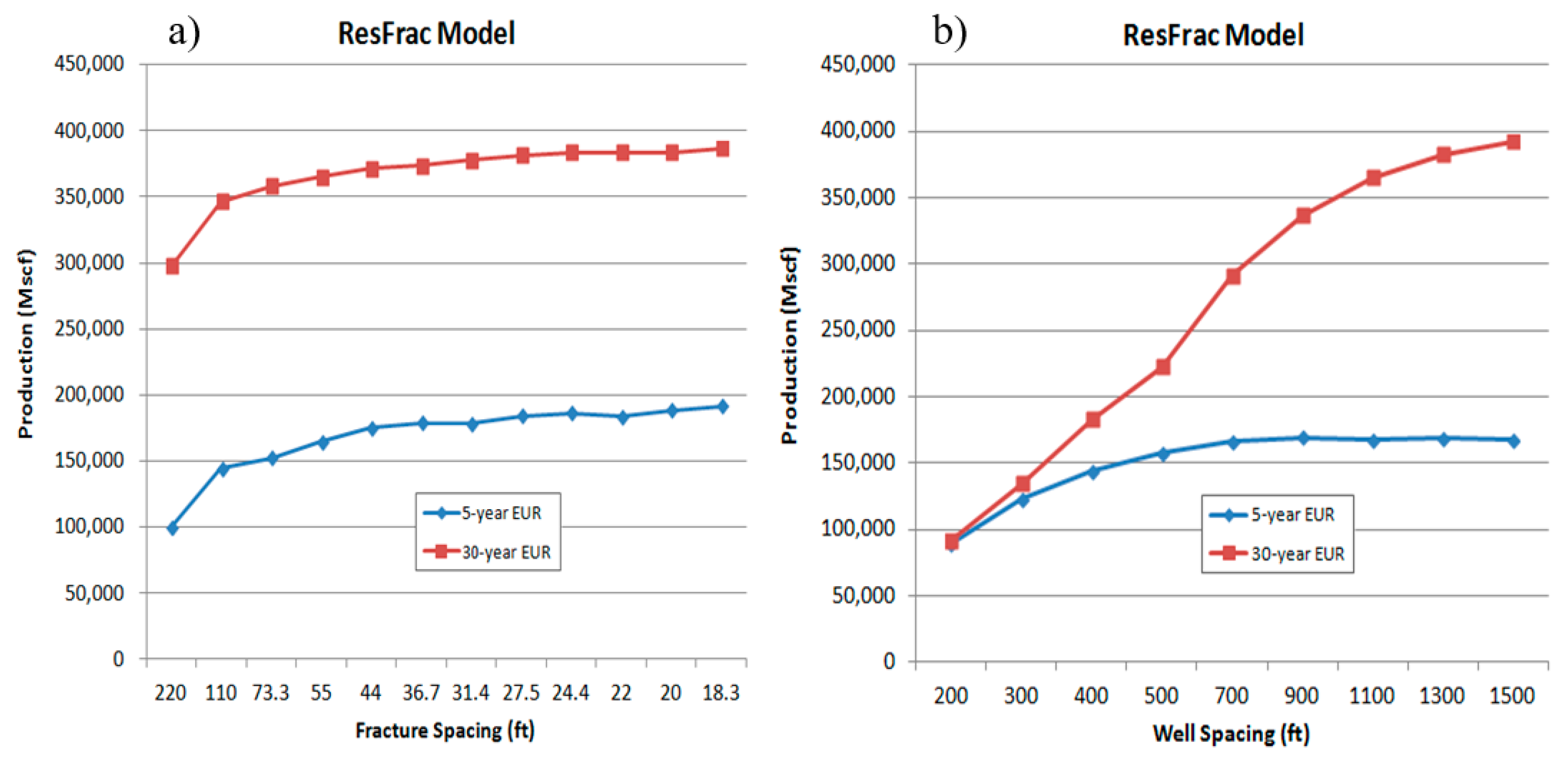
2.2. Numerical Reservoir Simulator (High Permeability Case)-Sensitivity to Fracture Spacing

The Utica reservoir permeability may be ultra-low (10–20 nD), but such a low permeability is hard to conclusively measure, and alternative interpretations are possible, with an effective permeability being at least an order of magnitude higher; up to 850 nD was used in a suite of reservoir simulations by Fowler et al. [13]. The various matrix permeability assumptions result in considerable variation in estimations of the fracture half-lengths when obtained via Monte-Carlo-based history-matching of production data with the advanced ResFrac simulator [13].
Certain parameters are well-constrained, while others have higher uncertainty ranges. The aim of the history matching against field data [7,13] was to constrain the uncertain parameters based on Monte-Carlo simulation runs. For example, micro-seismic clouds suggest large fracture half-lengths ranging between 550 and 800 ft (depending on pumped treatment volumes). Using such fracture half-lengths in production rate, history-matched reservoir models would indeed indicate matrix permeability of about 25 nD [13]. However, when instead a larger matrix permeability of 850 nD is used, such as could be induced by the fracture treatment after the closure of non-propped fracture wings, the coupled fracture-treatment and production-history-matched reservoir model generated much shorter fracture half-lengths, of about 95 ft only [13].
The aim of the present study is not to repeat history matching of field data–the prior history-matching study of Fowler et al. [13] was taken as a starting point. A well rate sensitivity study to cluster spacing for a high permeability matrix case (850 nD) was included in Fowler et al. [13], varying the cluster spacing by dividing a 220 ft fracture treatment stage-length by integers ranging between 1 and 12 (Table 1). The base case completion corresponds to a well spacing of 1100 ft with 55 ft cluster spacing. Figure 3a,b show the fracture up- and down-spacing effects on the well performance. Figure 3a,b give the resulting variation in the well performance when the cluster spacing is changed as per Table 1. What stands out from Figure 3a,b is that future wet gas wells, if completed with narrower cluster spacing, would have higher initial rates. Similar results were generated in earlier studies with flow-cell models (verified with CMG and KAPPA numerical simulators) for dry gas wells [12], and for black oil wells [9,10,11].
The simple reason for the predicted faster accumulation of production of a new well with fracture spacing (DN) narrower than the spacing of the type well (DT), is that the new wells have steeper pressure gradients at early times (Figure 4a–c). The pressure profiles (Figure 4c,d) are taken perpendicular to (and between) two adjacent hydraulic fractures, across the flow stagnation points (yellow dots), where the pressure profile has a saddle. However, the early gains in production rate for the well with narrow fracture spacing (Figure 4b) will be lost later, because the pressure gradients in the box space with the narrower spaced hydraulic fractures will flatten faster (Figure 4d). The cross-over of production rates is actually seen in the daily production rate plot of Figure 3b. In the cumulative (Figure 3a), one observes the wells with lower initial production rates (wider fracture spacing) will continue with still reasonable growth later in the well life. In contrast, the wells (or well sections) with narrowly spaced fractures will exhibit more quickly a leveling off of the cumulative production curve (Figure 3a). The field data for Well 2H had 825 ft well spacing, but 1100 ft well spacing (having model space width boundaries 1100 ft apart, or 550 ft at either side of the model well) was used in the history match for the same well (which is probably where the operator’s currently preferred well spacing lies).
The sensitivity of well performance to fracture spacing and well spacing distance for a relatively high permeability assumption (850 nD base case) are given in Section 2.2 and Section 2.3, respectively. Complementary sensitivity analyses for an ultralow permeability assumption (25 nD base case) are given in Appendix A.

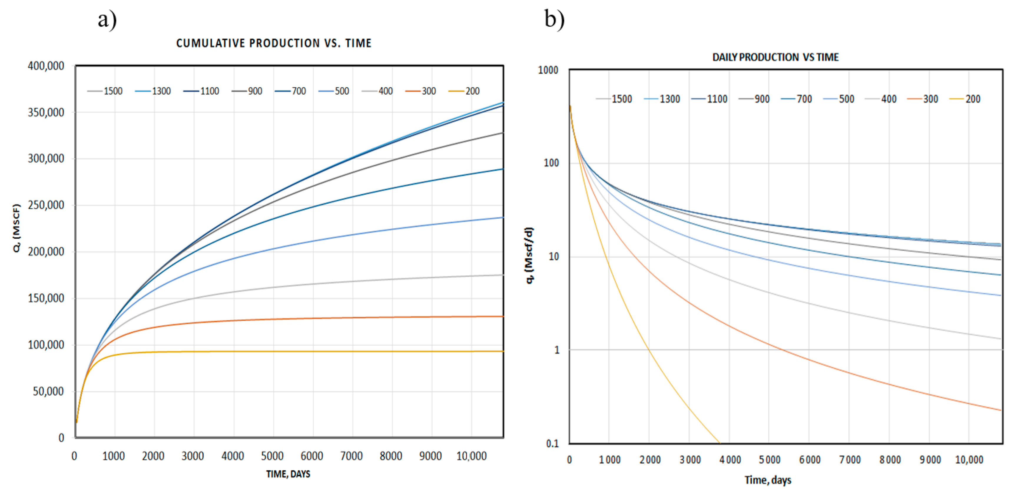
2.3. Sensitivity to Well Spacing: ResFrac Model

The sensitivity of well productivity to well-spacing changes has also been investigated with the ResFrac numerical reservoir simulator [13]. Figure 5a,b show the effect of well-spacing changes, while keeping the 55 ft base-case cluster-spacing the same for all wells. What stands out for the production curves for various well spacing is that all wells start out with the same initial rate. This is because all wells were assumed completed with the 55 ft base-case fracture spacing. However, the wells with a narrower inter-well distance will suddenly start to decline faster (Figure 5b). The data point where the narrowly spaced wells leave the decline curve trend of the well with the largest inter-well spacing was coined the kick-off point [9,11]. For a given well spacing, there is only one kick-off point, which occurs at a given time in the life of the well, the so-called kick-off time.
The kick-off time marks a profound moment in the well life, corresponding to the time that the pressure transient has discovered the neighboring well(s), which is when True Boundary-Dominated Flow (TBDF) starts. The change in the decline rate is due to a change in flow regimes from secondary transient to secondary BDF [14]. Theoretically, TBDF would correspond to terminal decline with an exponential decline curve (b = 0; see review in Reference [4]). However, a detailed analysis of b-values for hydraulically fractured oil and gas wells in late well-life will have b-values closer to 0.5 [15].
The timing of the kick-off point occurrence in the well life (so-called kick-off time) follows from the depth of investigation formula for the diffusive pressure transient [16] and Figure 13 in Reference [11]. The depth of investigation (ri) refers to the advance of the pressure draw-down front, which expands from the fracture tip outward. The transient radius of investigation, ri, at time t, varies with the reservoir properties (porosity, ϕ ( z ) and permeability, k ( z ) , fluid viscosity, μ, and compressibility, ct):
r i ( t ) = k ( z ) t 1688.7 ϕ ( z ) μ c t           [ ft ]
The time corresponding to the ‘discovery’ of a nearby well, marking the advent of True Boundary Dominated Flow (BDF), is given by equating ri equal to the distance to the interwell drainage boundary (IDB):
t = r i 2 ( t ) 1688.7 ϕ ( z ) μ c t k ( z )           [ s ]
The timing of the onset of True BDF will vary with well spacing W. The distance to IDB will be W/2, so setting ri = W/2 solves for the kick-off time. According to Equation (2), kick-off time is reached earlier for wells with narrower well spacing, which concurs with what is observed in Figure 5b. The flow-cell model (see Section 3) can be calibrated to predict with high confidence (>0.95 certainty) the well-performance after kick-off time (and the onset of TBDF) by adopting a two-segment decline curve. The second segment of the DCA curve starts at the kick-off point; the b-values follow from an empirical curve (see Figure A7 in Reference [11]).

2.4. Reservoir Simulator Results (High Permeability Case)

One of the principal aims to generate the production performance curves for wells with variable completion parameters and well spacing is to investigate the impact on the EUR accumulation. The variation of 5-year and 30-year EURs (Mscf), as forecasted by the ResFrac integrated simulator for wells with fracture spacing varying between 220 and 18.3 ft, are graphed in Figure 6a. The corresponding EURs after 5 and 30 years of production, are given in Table 2.
Similarly, the 5-year and 30-year EURs (Mscf), as forecasted by the ResFrac integrated simulator for wells with well spacing varying between 200 and 1500 ft, are graphed in Figure 6b. The corresponding EURs, after 5 and 30 years, are given in Table 3. Clearly, the 200 ft well spacing effectively drains the entire rock volume up to the inter-well drainage boundary in under five years, such that the 5-year and 30-year EUR are nearly the same. For well spacing larger than 900 ft, the 5-year EUR is no longer growing, but 30-year EURs continue to show a moderate increase. However, given the time value of money, well spacing larger than 900 ft does not make sense from an economic point of view, unless an operator wants to create room for future infill wells with minimal interference effects. If that is the case, then well spacing should be fixed at about 1200 ft.

3. Flow-Cell Model Results: Fracture-Spacing Effects

This section first explains the basic assumptions used in the flow-cell based production-forecast model (Section 3.1), then proceeds to give the key algorithms (Section 3.2), as developed in prior studies [9,10,11]. For the application to the Utica wet gas window, the selection of the type-curve well is outlined (Section 3.3), followed by flow-cell based DCA curves for Utica wells with varying fracture spacing calibrated with the ResFrac simulator results (Section 3.4). The flow-cell based 3-year and 5-year EURs are compared with those estimated previously in the ResFrac simulations of Section 2.3.

3.1. Basic Assumptions

In the flow-cell model, an array of elementary flow cells feeds mobile reservoir-fluid to the well via the transverse hydraulic fractures (Figure 1). The reservoir fluid is drained from both the fracture-box space and wing space, with the fracture-box space being pressure depleted early in the well history as was visualized in detail in earlier studies [9,14]. In the flow-cell model, the rate of the well, q W E L L ( t ) , at any one time, t, is controlled by the combined number of flow cells, N (combining Equations (8) and (9) in Reference [10]):
q W E L L ( t ) = N e ˙ y y ( t ) ϕ ( 1 R s ) B D H L           [ m 3 · s 1 ]
All flow cells are assumed to have identical global physical flow properties, and no heterogeneities may occur (i.e., uniform scalar permeability and constant fluid properties are assumed). Equation (3) further assumes that all flow cells (in the well’s array of elementary flow cells) have equal dimensions (with lengths D , H , L as defined in Figure 1). Changes in volume of produced fluid appearing at the surface relative to the reservoir level outflow point in the well are accounted for by the formation volume factor B. The pore space fraction of the total rock volume is given by ϕ . Volumetric constraints, due to the porous structure of the reservoir space and residual fluid not participating in the flow (as a fraction of total fluid) are given by R s . Additionally, the effectively propped fracture segments are assumed as the same for all fractures. Stage spacing is irrelevant for our analysis, as the stages feature in the completion process to deliver the pressures required to create the hydraulic fractures. Each perforation cluster is assumed to generate identical, successfully propped hydraulic fractures (i.e., infinite conductivity is achieved over the stated half-length).
The well rate decline depends on the intrinsic rate, e ˙ 1 ( t ) = e ˙ x x ( t ) = e ˙ y y ( t ) , of the cumulative elementary flow cells, and vice versa (Figure 1), which can be scaled by any type well (Equation (9) in Reference [10]):
e ˙ y y ( t ) = q T Y P E _ W E L L ( t ) B N ϕ ( 1 R s ) 1 D T H T L T           [ s 1 ]
The intrinsic reservoir properties like permeability, fluid viscosity, and initial reservoir pressure need not be known for further modeling, as these are all scaled by the intrinsic rate e ˙ 1 ( t ) = e ˙ x x ( t ) = e ˙ y y ( t ) of the elementary flow cells, which is computed using the known completion design parameters ( D T , H T , L T ) from a type well. The type well production rate, q T Y P E _ W E L L ( t ) , is required to scale the intrinsic e ˙ y y (t) for the target zone by history-matching early production data. Porosity and permeability are assumed static over the field life, e.g., no stress sensitivity occurs.
The reservoir fluid in the original flow-cell model [9,10] was assumed to be single phase oil and incompressible, such that PVT effects can be ignored. However, for wet gas wells, such an assumption will no longer hold, but the model appears to hold up when correction factors are introduced to account for PVT effects (see Section 3.4). The model further assumes that liquid loading by condensate/water mixtures–common in reservoirs with high movable water saturation that may complicate lift of the gas and kill the well [17,18]–does not occur during the life of the well. However, condensate banking near the wellbore is accounted for in the ResFrac simulation. If condensates form near the fracture planes and in depletion zones near the wellbore, then a reduction of fracture spacing may lead to gas faster reaching the dew-point pressure, and the build-up of condensates will depress gas rates to the well, and may result in the tighter well-spacing being counterproductive.

3.2. Key Algorithms

As long as the BHP in the new well is identical to that used in the parent well, the effect of fracture spacing and related changes in the dimensions of the elementary flow cell ( D N , H N , L N ) on the initial flow rate relative to the type curve well is given by (Equation (15) in Reference [10]):
q i _ N e w W e l l q i _ T y p e W e l l = V R N N D N N T D T ( D T D N ) 2
The production rate of the new well is given by a hyperbolic equation:
q ( t ) = q i _ N e w W e l l ( 1 + b N D i _ N t ) 1 b N
The various parameters used in Equation (5) can be obtained as follows:
b N = 1 N N D N N T D T ( V R D T D N ) 2 D i _ T D i _ N ( 1 b T )
D i _ N = D i _ T V R N T D T N N D N ( D T D N ) 2.5
V R = V N V T = N N D N L N H N N T D T L T H T
The production performance of future wells may now be predicted by substituting in Equation (6) the required q i _ N e w W e l l (Equation (5)), b N (Equation (7)), and D i _ N (Equations (8) and (9)), based on the hyperbolic decline curve for a type curve well (which solves for b T and D i _ T ).
If the spacing of the fractures in a new well, D N , is different from the fracture spacing in the type well, D T , but wells have the same total length, then the fracture spacing times the number of fractures in each type of well ( N T D T , N N D N ), will be the same N T D T = N N D N . However, expressions (5)–(9) account for differences in both well spacing and overall well length, as well as for differences in (if any) fracture half-length, fracture height, and fracture spacing. Note that double the fracture half-length was used to denote L (see inset sketch in Figure 1).

3.3. Type-Well Selection

The type well used for the flow-cell model is Utica Well 2H in the wet gas window (Section 2.1) for which 15 months historic production data was available. Recall that Well 2H was also used for the history matching with a long-term production curve by the ResFrac simulator [13]. In a standard flow-cell model approach, historic field data are matched by a DCA curve to obtain a long-term production forecast type curve for the base case.
However, in the case of Well 2H, the historic production data were spurious. Flow-back and possibly compressibility effects resulted in the well not showing a clear production-rate decline-trend until after the 8th/9th month of production. If negative b-values are not excluded in the solver settings, the DCA regression returns a negative b-value (Figure 7). The negative b-value results in a hyperbole that is concave downward, instead of concaving up, as one would normally see. This result is not tenable for a long-term DCA forecast, but is purely a result of fitting against a limited historic data-set without omitting the first couple of months with non-declining data.
If negative values in solver solutions for decline parameters Qi, Di, and b are excluded in the DCA regression procedure illustrated in Figure 7, then the historic data for Well 2H will return b = 0. Acceptance of the b = 0 DCA fit would be an equally poor engineering judgment, because hydraulically fractured gas wells are known to stay in transient flow for prolonged times, hence b > 1 at early times.
To end up with a realistic type curve for the flow-cell model, the Resfrac pressure history matched base curve was adopted for Well 2H (Figure 8a). The data from the realization in Figure 8a were subsequently used to match a hyperbolic decline curve to the interpolated production data for the first 40 months (Figure 8b). The history matched DCA parameters are Qi = 787 Mcf/day, Di = 13.597/year (nominal rate), and b = 1.596.

3.4. Fracture-Spacing Effects with Flow-Cell Model

The DCA type curve (Figure 8b) was used as a starting point for the flow-cell model-based production forecasts, using the algorithms given in Section 3.2 and with the basic assumptions of Section 3.1 in place. A satisfactory fit with the ResFrac sensitivity curves for fracture spacing changes (Figure 3a,b) could be obtained after introducing additional adjustment factors, as follows. The production rate of the new well, for oil and dry gas wells given by Equation (6), for wet gas wells needs an adjustment factor qi_adj to account for PVT effects:
q ( t ) = q i _ a d j ( q i _ N e w W e l l ) ( 1 + b N D i _ N t ) 1 b N
Similarly, the nominal decline rate of the new well, for oil and dry gas wells is given by Equation (8), which for wet gas wells needs an adjustment factor Di_adj:
D i _ N = D i _ a d j ( D i _ T V R N T D T N N D N ) ( D T D N ) 2.5
The adjustment factors qi_adj and Di_adj of Figure 9a,b were determined by finding the best matches against the ResFrac results. Table 4 gives the corresponding empirical values of the adjustment factors qi_adj and Di_adj. The physical interpretation of the required repairs of the standard flow-cell algorithms model for use in wet gas reservoirs is that the two adjustment factors account for the wet gas compressibility effects occurring in the reservoir space drained by Well 2H.
Figure 10a,b show the fracture up- and down-spacing effects on the well performance according to the calibrated flow-cell model; the fracture spacing changes are again as assumed in Table 1. The corresponding ResFrac simulator forecasts were given in Figure 3a,b. There is a satisfactory match between ResFrac forecasts (Section 2.2) and the flow-cell based forecasts of fracture-spacing effects on well productivity (Section 3.4). For example, the 5-year and 30-year EURs graphed for the flow-cell model in Figure 11a match closely with the ResFrac EUR results graphed in Figure 6a. The flow-cell EUR data are given in Table 5 for direct comparison with the ResFrac data in Table 2a. The mismatch, Δ, is here defined as:
Δ = EUR _ Flow - Cell EUR _ ResFrac 1
The mismatch between the EUR estimates of the flow-cell model and the ResFac simulator is separately graphed in Figure 11b. Our conclusion is that the 5-year EUR estimates of the flow-cell model are within 92–99% of the ResFrac EUR estimates, and the 30-year EUR estimates of the flow-cell model are all within a 97% confidence range of the ResFrac model results.

4. Flow-Cell Model: Well-Spacing Effects

4.1. Well Pressure Interference Via the Matrix

The flow-cell model can also be used to predict the effect of well-spacing changes on the well rate performance and EURs. Finding the optimum well spacing, that does not leave valuable acreage undrained, is a challenging task for petroleum engineers. The reason is that overly tight well-spacing will reduce the overall volume that can be drained and will lead to rapid pressure draw-down of the matrix regions between adjacent wells [14]. In addition to the pressure-decline effect, hydraulic fractures of adjacent wells may connect during the fracture-treatment operation [19]. If permanent pressure communication is established, the two wells effectively represent an integrated production system [20], which predicts the well behavior more challenging [2,4].
The below analysis neglects fracture-hit effects. However, the flow-cell model can be adapted to predict the production performance (rate and EUR) when the well spacing of the new wells is narrower or wider than used for the prior type well, as was previously shown for oil wells [9,10,11].
Figure 12a,b show two distinct cases relevant for well spacing studies. The simple case is the parent-parent well-pair, which is when the adjacent wells are both drilled and completed at the same time (Figure 12a). The slightly more complex case is the parent-child well-pair (Figure 12b), which means the child well post-dates the parent well. Both cases can be modeled by the flow-cell model [9], which was adapted in the present study for application to wet gas wells.

4.2. Kick-off Times and Final Segment b-Values

The ResFrac study of well productivity sensitivity to well-spacing by Fowler et al. [13] was reviewed in Section 2.3. The results showed how the EUR for the 850 nD base-case well would change when the well spacing was varied between 200 and 1500 ft (Figure 6b and Table 3). All production curves start off with the same initial rate (Figure 5a,b), but when the pressure transient would discover the neighboring wells, the well rate would rapidly decrease. For oil wells, the analysis of the depth of investigation formula of Equation (2) gave excellent matches with the kick-off times of the rate curves generated with a KAPPA reservoir simulator [11].
In the present study of wet gas wells, the depth of investigation formula (Equation (2)), used with the key diffusivity parameters given in Table 6, gave kick-off times much shorter than predicted by the ResFrac model of Figure 5b. The ResFrac model kick-off times are graphed in Figure 13a, and were used as inputs in the flow-cell model to override the DOI formula generated kick-off times. However, using the approximate compressibility at the initial reservoir pressure, which for an ideal gas is 1/P, results in close matches between the DOI formula and ResFrac kick-off times.
Unlike the flow-cell model curves for fracture-spacing effects, which can all be matched by a single-segment DCA (for definitions, see Reference [15]), changes in the well rates, due to well-spacing effects require modeling with a 2-segment DCA approach [11]. The second segment of the DCA curve represents the well’s flow behavior after the pressure transient has discovered the drainage boundaries of the well’s flow space as limited by the no-flow inter-well drainage boundary (IDB; Figure 12a). Although True BDF would theoretically correspond to an exponential terminal decline, as originally proposed by Maley [21], our prior study [11] already demonstrated that the KAPPA-simulator results show no such exponential decline. Instead, a hyperbolic decline occurs, with a b-value smaller than for the first DCA segment. The ResFrac-simulator well-rate forecast of Figure 5b shows the same phenomenon: Terminal well-rates do not follow an exponential decline (which would occur as a straight line on log-rate versus linear-time plots).
The b-values for the second segment of the DCA curves are plotted in Figure 13b. The kick-off times of Figure 13a and b-values of Figure 13b allow the construction of flow-cell based forecast for well-spacing sensitivity by 2-segment DCA curves. The first segment b-value (1.596) was the same as used for the type curve (Section 3.3) used in the fracture-spacing study of Section 3.

4.3. Well-Spacing Effects with Flow-Cell Model

Figure 14a,b show the effects on the well performance of well-spacing changes according to the calibrated flow-cell model. The corresponding ResFrac simulator forecasts were given in Figure 3a,b. There is a satisfactory match between the flow-cell and ResFrac forecasts of well spacing effects on well productivity. For example, the 5-year and 30-year EURs graphed in Figure 15a match closely with the ResFrac EUR results graphed in Figure 6b. The flow-cell EUR data are given in Table 7 for direct comparison with the ResFrac data in Table 3. The mismatch, Δ (of Equation (12)), between the EUR estimates of the flow-cell model and the ResFac simulator is separately graphed in Figure 15b.
Our conclusion is that the 5-year EUR estimates of the flow-cell model are within 94% of the ResFrac EUR estimates, and the 30-year EUR estimates of the flow-cell model are all within a 93% confidence range of the ResFrac model results.

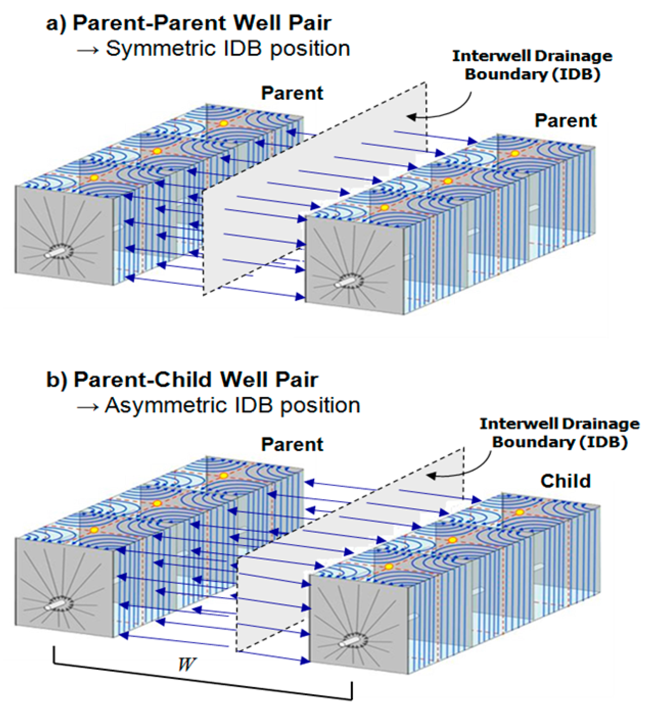
4.4. Well-Spacing Effects (Parent-Child Wells)

A prior study has analyzed in considerable detail the shift in the position of the IDB of the parent well when a child well is introduced [9]. The curves are given in Figure 14a,b also predict the future behavior of the parent well, if one realizes that a parent well will encounter a kick-off point time as determined by the distance of the changing IDB when a child well is suddenly introduced. Clearly, assuming no fracture hits occur, the flow rate of the parent well will still be adversely affected by the sudden appearance of a nearby child well, which will create a new IDB in closer proximity to the parent well (Figure 13b).
All wells in a given reservoir start with the same rate if fracture treated in the same manner as the type curve well, which is valid as long as the child well is not drilled late in the life of the parent well (see Figure 19a in Reference [9]). The child well will discover its own distance to the IDB, and therefore, its behavior is also captured in Figure 14a,b, with the understanding that the effective well-spacing factor for the child well is given by twice the distance to its IDB.

5. Discussion

The significance of being able to generate production performance-forecasts curves for undrilled wells (PUDs) with a flow-cell model is that the resulting DCA curves are fully described by analytical expressions. The expressions are suitable for computation in a spreadsheet template, which can be coupled with a cash flow analysis to evaluate which fracture spacing (or fracture length, height, overall well length) and well-spacing will give the optimum net present value (NPV) and internal rate of return (IRR), as was demonstrated before in a case study for Eagle Ford acreage [10]). The prior study also showed that the actual optimum may shift considerably with assumed commodity prices and D&C costs. Our conclusion is that rapid NPV and IRR optimization with a suite of flow-cell based spreadsheets provides operators with a practical tool for quick assessment of field development decisions regarding drilling and completion design solutions. Further details are discussed below.

5.1. Merits of Reserves Reporting Based on Flow-Cell Model

For operators of shale acreage, the accurate reporting of proven developed and proven undeveloped reserves is important for (1) compliance with reserves reporting guidelines, as well as for (2) reserves-based lending to finance ongoing field development efforts. The discounted value of the proven reserve volumes provides companies with collateral for debt financing in so-called reserves-based lending [22]. Oil and gas operators of shale leases hold a reserves inventory comprised of various uncertainty ranges: Proven (P90), probable (P50 minus P90), and possible (P10 minus (P50 + P90)) volumes. The P10, P50, and P90 qualifiers refer to the volume estimations likelihood with 10%, 50%, and 90% that the stated volumes can be extracted. Only the P90-volumes may be referred to as proven reserves, following the probabilistic definition of the US Securities and Exchange Commission (SEC). At the time of the reserves reporting date, the proven reserves (P90) all exist with at least 90% certainty, and the so-called unproven part of the reserves (probable plus possible volumes) gives a future upside.
Despite being confined to P90 reserves volumes to jumpstart the financing of development projects in unconventional acreage, operators can typically build and report–under current SEC guidelines–enormous proven reserve volumes with relatively little upstart capital. Initial capital expenditures will only have to be made for wells that are either (1) drilled and completed, thus producing, or (2) drilled but left uncompleted (DUCs), thus non-producing. Both categories represent P90 reserves and add to the reserves-based lending collateral. In addition to the so-called proven developed reserves (made up by the producing and non-producing wells), operators may further claim as P90 collateral (3) the so-called proved undeveloped reserves (PUDs).
The attractiveness of PUD reserves being included in P90 reserves-based lending collateral is that no direct capital expenditure has to be made by the company–it is simply sufficient to pledge that the development investment will be made within the next five years [23]. For the PUDs to be booked compliant with SEC reserves reporting guidelines, US shale plays companies are regulated–and occasionally audited–by the SEC. Among the SEC requirements are having in place a final investment decision (FID) for the development–within the next five years–of the PUD assets [23], typically for infill-well locations in unconventional acreage. The FID letters and lease titles must exist in the company files for reported reserves. Such documented proven undeveloped reserves (PUDs) have the same status for reserves-based lending as the proven developed reserves; all reserves must be feasible and economically viable with current technology.
Because of the economic importance for operators to accurately estimate the PUD reserve volumes (under the current year 12-month-averaged product prices and company cost), rapid assessment methods are of immense value to oil and gas companies. To estimate the production delivered by future–as of yet undeveloped–wells (PUDs), companies presently may use various methods. These methods range from applying a production type curve based on analogy to nearby wells [24], via data analytics [6], to full reservoir models [2,4,13]. The flow-cell model offers shale operators a fast, benchmarked method to predict the performance of infill wells with changes in fracture treatment design parameters, well spacing, and total well length.

5.2. Back-Casting Completion Failures

The fracture spacing used in our analysis does not take into account any imperfections in the completion process. That is, each perforation cluster was assumed to create one principal fracture, and all fractures are created equal. The flow-cell model has previously been verified for use in black oil wells [9,10,11] and dry gas wells [12] with numerical reservoir models (CMG, KAPPA). Comparison of the forecasts made by both the numerical and the flow-cell models (which were closely matched, and thus, both reliable for an ideal well system) with actual well performance revealed that about 25% of the perforation clusters seemed to have failed when back-casting the flow-cell model to history match actual well performance [12].
The verification of the flow-cell model, therefore, best occurs via noise-free numerical models, which in the present wet-gas study is a numerical ResFrac-simulator that first matched a type curve for Well 2H in Figure 8b. Due to the noise in field well data, caused by operational issues (well work-over) and failed perforations, use of the flow-cell model without prior validation and calibration with an independent simulator of a physically perfect well system, is not recommended. Although the original flow-cell-model equations work accurately for oil and dry-gas wells with empirical type curves using field data only, field validation after new wells have actually been drilled may discover again that the flow-cell model, which assumes that all perforations result in equally propped hydraulic fractures that are perfectly draining each flow cell, needs downward adjustments to discount the well rate for the failed perforations.
The recovery factor RFN of new wells can be quickly assessed based on the hydrocarbons in place (OGIP) estimations, and for different well spacing should be based on the volume given by N*D*H*(WN/2), with new well spacing WN. The shortcut version for OGIP estimations is using the ratio WN/WT when well spacing changes, but N*D*H are unchanged (see Figure 1 for dimensions). The new well’s RFN = EURN/[OGIP for N*D*H*(WN/2)].

5.3. Strengths and Weaknesses of the Flow-Cell Model

The flow-cell model was designed for use in (nearly) incompressible reservoir conditions (see assumptions in Section 3.1). When used for production forecasting of wet gas wells, compressibility changes with reservoir pressure, and the viscosity of the gas also changes with pressure (which drops when reservoir depletion advances). By calibrating with the ResFrac simulator, correction factors were introduced in the flow-cell model equations (Section 3.4), which corrected the analytical solutions such that the model results still match the numerical forecasts by the ResFrac simulator for wet-gas wells with high confidence (>0.92) for all cases, that is fracture-spacing sensitivity (Figure 11b) and well-spacing sensitivity (Figure 15b). A weakness of the flow-cell model is that it requires calibration with noise-free reservoir-simulator results (CMG, KAPPA, ResFrac).
A strength of the flow-cell model is that it helps to quantify how physical processes in the reservoir (such as pressure interference in between fractures and between wells) will affect the well rate. An already stated strength (Section 5.1) is that the validated model can be used to optimize field development decisions by coupling those decisions with rapid NPV and IRR computations in a spreadsheet environment, which can be used by anyone with basic engineering skills as opposed to running multiple numerical reservoir simulations, which requires advanced reservoir modeling skills. The use of numerical simulators is recommended in conjunction with fast and effective field-development decisions based on both reservoir physics and economic optimization.
In spite of its simple nature, the projection of production decline curves with analytical methods is still the single-most widely used method for forecasting production from unconventional oil and gas wells. The future production potential of the acreage is routinely assessed, making use of various DCA methods. The flow-cell model uses a 2-segment Arps hyperbolic decline model. Prior studies have argued that Arps would result in over-optimistic EUR estimations, and other DCA methods would be more accurate [25]. However, when the Arps hyperbolic solution method is used in a 2-segment DCA approach, as explained here, the optimistic bias of single-segment DCA disappears. The use of Arps hyperbolic DCA method is recommended, because of its reasonable fit accuracy and ease of use (e.g., References [26,27]).

6. Conclusions

Flow-cell based well-rate predictions were compared against those of the independent reservoir simulations. Unlike complex simulations, the spreadsheet-based analysis is much quicker. Once the flow rate from an existing well is available, the behavior of new infill wells can be predicted and improved by tweaking some aspects of the flow cells, such as the height, length, or spacing of hydraulic fractures and between wells. Furthermore, this type of analysis can be conducted before drilling the new wells so that oil and gas recovery from the lease region can be maximized. This is good news for shale operators, who need to forecast and improve the performance of the new wells that they plan to drill. Our spreadsheet-based flow-cell analysis has been tested against sophisticated reservoir simulators in a series of detailed studies [9,10,11,12], and the flow-cell model appears to be accurate enough for use in reserves estimations.
The flow-cell model has been adapted in the present study for use in wet-gas wells by introducing correction factors based on the calibration of well performance forecast with an independent ResFrac numerical reservoir-simulator. The adjusted flow-cell model can generate 2-segment DCA forecasts for future wells with changes in fracture spacing and well spacing that match the numerical forecasts with 0.92 accuracy or higher. The flow-cell model, thus, provides a valuable, practical tool for operators to generate physics-based DCA curves to forecast monthly production rates of undrilled wells for the estimation of proven undeveloped reserves (PUDs).
The PUDs generate reserves without the necessity of immediate capital expenditure, and can be used as collateral for reserves-based lending such that the wells can actually be drilled in the near future. Procuring reliable estimations of PUDs as a basis for reserves-based lending is particularly relevant in the current regime with restricted access to capital in the global financial markets.

Funding

This project was sponsored by the Crisman-Berg Hughes consortium and startup funds from the Texas A&M Engineering Experiment Station (TEES).

Acknowledgments

ResFrac CEO Mark McClure and reservoir engineer Garrett Fowler provided primary data and reservoir simulator results used in this study. They also participated in various detailed discussions related to clarifying integration of ResFrac results with the contents of the present work.

Conflicts of Interest

The author declares no conflict of interest.

Appendix A. Numerical Reservoir Simulator Results (Low Permeability Case)

Another set of well performance forecasts was generated for the low permeability assumption (25 nD), where each realization for a different spacing of the fracture clusters would results in a different fracture geometry, commonly non-symmetric about the wellbore and with irregular shapes (Figure A1). The effective fracture spacing is about 100 ft for the 25 nD base case.
A study of well rate sensitivity to cluster spacing for the low permeability case (25 nD) was included in Fowler et al. [13], varying the cluster spacing by dividing a 220 ft fracture treatment stage-length by integers ranging between 1 and 12 (Table 1). The fracture spacing sensitivity is plotted in Figure A2a,b.
Figure A1. Perspective view of 3-well fracture creation model in low-perm matrix model, accounting for stress shadowing, leading to asymmetric hydraulic fracture development. The middle well is Well 2H with fracture conductivity used as base case inputs for the ResFrac production forecast curves of Figure A2 and Figure A3.
Energies 13 06736 g0a1
Figure A2. Production performance of Utica wells for fracture spacing ranging between 220 and 18.3 ft. The base case performance is for the Utica type well with 55 ft fracture spacing. The impact of wider and narrower fracture spacing on well productivity is graphed for both (a) the cumulative, and (b) daily production rates. Well performance curves were generated with a numerical reservoir simulator by ResFrac (data from Reference [13]).
Energies 13 06736 g0a2
The sensitivity of well performance to well spacing distance for the 25 nD base case is given in Figure A3a,b. A comparison of the graphs for low permeability cases (Figure A3) and high permeability cases (Figure 5) shows that, for the high permeability realizations, all wells start out with the same basic flow rate, but then decline sets in faster (from the kick-off points) as was separately observed in earlier flow-cell models calibrated with CMG simulations [10,12] and KAPPA simulations [9,11].
However, in the low permeability cases (Figure A3), the wells very quickly start out with different initial rates. The explanation is that for each well spacing realization for the low perm cases, the ResFrac simulator runs a new simulation for hydraulic fracture growth. The result is that in the simulations of Figure A3, not only varies the well spacing, but also the fracture spacing and fracture geometry will be different for each well realization. Henceforth, the distinct kick-off points that are characteristic for well spacing change graphs (e.g., Figure 5, and similar graphs in prior flow-cell studies, such as Figure 14 in Reference [11]) are not observed for the low-perm ResFrac realizations of Figure A3, presumably overshadowed by other effects, due to fracture geometry variations.
Figure A3. Production performance of Utica wells for well spacing ranging between 300 and 2300 ft. The base case performance is for the Utica type well with 55 ft fracture spacing and an assumed 1100 ft well spacing. The impact of wider and narrower well spacing on well productivity is graphed for both (a) the cumulative, and (b) daily production rates. Well performance curves were generated with a numerical reservoir simulator by ResFrac (data from Reference [13]).
Energies 13 06736 g0a3

References

  1. Izadi, G.; Guises, R.; Barton, C.; Randazzo, S.; Mahrooqi, S.; Shaibani, M.; Dobroskok, A. Advanced Integrated Subsurface 3D Reservoir Model for Multistage Full-Physics Hydraulic Fracturing Simulation. In Proceedings of the International Petroleum Technology Conference, Dhahran, Saudi Arabia, 13–15 January 2020. [Google Scholar] [CrossRef]
  2. Yu, W.; Xu, Y.; Weijermars, R.; Wu, K.; Sepehrnoori, K. A numerical model for simulating pressure response of well interference and well performance in tight oil reservoirs with complex fracture geometries using the fast embedded discrete fracture model method. SPE Reserv. Eval. Eng. 2018, 21, 489–502. [Google Scholar] [CrossRef]
  3. Garza, M.; Baumbach, J.; Prosser, J.; Pettigrew, S.; Elvig, K. An Eagle Ford Case Study: Improving an Infill Well Completion through Optimized Refracturing Treatment of the Offset Parent Wells. In Proceedings of the SPE Hydraulic Fracturing Technology Conference and Exhibition, The Woodlands, TX, USA, 5–7 February 2019. [Google Scholar] [CrossRef]
  4. Yu, W.; Wu, K.; Zuo, L.; Tan, X.; Weijermars, R. Physical Models for Inter-Well Interference in Shale Reservoirs: Relative Impacts of Fracture Hits and Matrix Permeability. In Proceedings of the SPE Unconventional Resources Technology Conference, San Antonio, TX, USA, 1–3 August 2016. SPE-URTeC 2457663. [Google Scholar] [CrossRef] [Green Version]
  5. SPE Taskforce Final Report, 2016. Unconventional Reserves Task Force, The Woodlands, TX, USA, 18–19 August 2015. Available online: https://www.spwla.org/Documents/SPWLA/TEMP/Unconventional%20Taskforce%20Final%20Report.pdf (accessed on 13 December 2020).
  6. Zhao, P.; Dong, R.; Liang, Y. Regional to Local Machine-Learning Analysis for Unconventional Formation Reserve Estimation: Eagle Ford Case Study; Society of Petroleum Engineers: Houston, USA, 2020. [Google Scholar] [CrossRef]
  7. Cipolla, C.; Gilbert, C.; Sharma, A.; LeBas, J. Case History of Completion Optimization in the Utica; Society of Petroleum Engineers: Houston, TX, USA, 2018. [Google Scholar] [CrossRef]
  8. McClure, M.; Picone, M.; Fowler, G.; Ratcliff, D.; Kang, C.; Medam, S.; Frantz, J. Nuances and Frequently Asked Questions in Field-Scale Hydraulic Fracture Modeling. In Proceedings of the SPE Hydraulic Fracturing Technology Conference and Exhibition, The Woodlands, TX, USA, 4–6 February 2020. [Google Scholar] [CrossRef]
  9. Weijermars, R.; Tugan, F.M.; Khanal, A. Production Rates and EUR Forecasts for Interfering Parent-Parent Wells and Parent-Child Wells: Fast Analytical Solutions and Validation with Numerical Reservoir Simulators. J. Pet. Sci. Eng. 2020, 190, 107032. [Google Scholar] [CrossRef]
  10. Weijermars, R.; Khanal, A. Production Interference of Hydraulically Fractured Hydrocarbon Wells: New Tools for Optimization of Productivity and Economic Performance of Parent and Child Wells. In Proceedings of the SPE Europec featured at 81st EAGE Conference and Exhibition, London, UK, 3–6 June 2019. SPE-195544-MS. [Google Scholar]
  11. Weijermars, R.; Nandlal, K. Pre-Drilling Production Forecasting of Parent and Child Wells Using a 2-Segment DCA Method Based on an Analytical Flow-Cell Model Scaled by a Single Type Well. Energies 2020, 23, 1525. [Google Scholar] [CrossRef] [Green Version]
  12. Waters, D.; Weijermars, R. Predicting the Performance of Undeveloped Multi-Fractured Marcellus Gas Wells Using an Analytical Flow-Cell Model (FCM). Energies 2021. work in review. [Google Scholar]
  13. Fowler, G.; McClure, M.; Cipolla, C. A Utica Case Study: The Impact of Permeability Estimates on History Matching, Fracture Length, and Well Spacing. In Proceedings of the SPE Annual Technical Conference and Exhibition, Calgary, AB, Canada, 30 September–2 October 2019. [Google Scholar] [CrossRef]
  14. Weijermars, R.; Nandlal, K.; Khanal, A.; Tugan, M.F. Comparison of Pressure Front with Tracer Front Advance and Principal Flow Regimes in Hydraulically Fractured Wells in Unconventional Reservoirs. J. Pet. Sci. Eng. 2019, 183, 106407. [Google Scholar] [CrossRef]
  15. Tugan, M.F.; Weijermars, R. Variation in b-sigmoids with flow regime transitions in support of a New 3-Segment DCA Method: Improved Production Forecasting for tight oil and gas wells. J. Pet. Sci. Eng. 2020, 192, 107243. [Google Scholar] [CrossRef]
  16. Weijermars, R.; Nascentes Alves, I. High-Resolution Visualization of Flow Velocities Near Frac-Tips and Flow Interference of Multi-Fracked Eagle Ford Wells, Brazos County, Texas. J. Pet. Sci. Eng. 2018, 165, 946–961. [Google Scholar] [CrossRef]
  17. Tugan, M.F. Deliquification techniques for conventional and unconventional gas wells: Review, field cases and lessons learned for mitigation of liquid loading. J. Nat. Gas Sci. Eng. 2020, 83, 103568. [Google Scholar] [CrossRef]
  18. Weijermars, R.; Nandlal, K.; Tugan, M.F.; Dusterhoft, R.; Stegent, N. Hydraulic Fracture Test Site Drained Rock Volume and Recovery Factors Visualized by Scaled Complex Analysis Models: Emulating Multiple Data Sources (production rates, Water Cuts, Pressure Gauges, Flow Regime Changes, and b-sigmoids). In Proceedings of the Unconventional Resources Technology Conference, Austin, TX, USA, 20–22 June 2020. URTeC 2020–2434. [Google Scholar]
  19. Sukumar, S.; Weijermars, R.; Nascentes Alves, I.; Noynaert, S. Analysis of Pressure Communication between Austin Chalk and Eagle Ford Wells during a Zipper Frac Operation. MDPI Energies—Special Issue: “Improved Reservoir Models and Production Forecasting Techniques for Multi-Stage Fractured Hydrocarbon Wells”. Energies 2019, 12, 1469. [Google Scholar] [CrossRef] [Green Version]
  20. Yang, X.; Yu, W.; Weijermars, R.; Wu, K. Fracture hits via diagnostic charts to assess production interference level. SPE J. 2020, 1–27. [Google Scholar] [CrossRef]
  21. Maley, S. The Use of Conventional Decline Curve Analysis in Tight Gas Well Applications. In Proceedings of the SPE/DOE (Society of Petroleum Engineers and U.S. Department of Energy), Low Permeability Gas Reservoirs, Denver, CO, USA, 19–22 May 1985. [Google Scholar] [CrossRef]
  22. Weijermars, R.; Johnson, A.; Denman, J.; Salinas, K.; Kennedy, M.; Williams, J. Creditworthiness of North American Oil Companies and Minsky Effects of the (2014–2016) Oil Price Shock. J. Financ. Account 2018, 6, 162–180. [Google Scholar] [CrossRef]
  23. Weijermars, R. Jumps in Proved Unconventional Gas Reserves Present Challenges to Reserves Auditing. SPE Econ. Manag. 2012, 4, 131–146. [Google Scholar] [CrossRef]
  24. SPEE Monograph 3. Guidelines for the Practical Evaluation of Undeveloped Reserves in Resource Plays; Society of Petroleum Evaluation Engineers: SPE Houston, TX, USA, 2011; Available online: https://spee.org/ (accessed on 13 December 2020).
  25. Mishra, S. A New Approach to Reserves Estimation in Shale Gas Reservoirs Using Multiple Decline Curve Analysis Models; Society of Petroleum Engineers: Houston, TX, USA, 2012. [Google Scholar] [CrossRef]
  26. Hu, Y.; Weijermars, R.; Lihua, Z.; Yu, W. Benchmarking EUR Estimates for Hydraulically Fractured Wells with and without Fracture Hits Using Various DCA Methods. J. Pet. Sci. Eng. 2017, 162, 617–632. [Google Scholar] [CrossRef]
  27. Tugan, F.M.; Weijermars, R. Improved EUR Prediction for Multi-Fractured Hydrocarbon Wells Based on 3-Segment DCA: Implication for Production Forecasting of Parent and Child Wells. J. Pet. Sci. Eng. 2020, 187, 106692. [Google Scholar] [CrossRef]
Figure 1. Principle sketch of the single elementary flow cell (inset). Blue lines are streamlines in flow cell between two sub-parallel hydraulic fractures. Main image: Three flow cells in partial section of a single horizontal well. Dashed lines are flow separation surfaces. Yellow dots are flow stagnation points (adapted from Reference [9]).
Energies 13 06736 g001
Figure 2. Map view of well layout (upper left) and location in the wet gas window of the Utica Shale Formation, Ohio (lower left). The right image shows map views of the collocated micro-seismic response clouds for the four outer wells in the Utica field test site (adapted from Reference [7]).
Energies 13 06736 g002
Figure 3. Well performance curves were generated for Utica wells with a numerical reservoir simulator by ResFrac for fracture spacing ranging between 220 and 18.3 ft (Table 1). The base case performance is for the Utica type well with 55 ft fracture spacing. The impact of wider and narrower fracture spacing on well productivity is graphed for both (a) the cumulative, and (b) daily production rates (data from Reference [13]).
Energies 13 06736 g003
Figure 4. Principle sketch of flow-cell model key aspects. (a) Map view of streamlines for type well and a new well with narrower fracture spacing. (b) Comparison of pressure depletion profiles along line x = 0 for both type well and new well: (c) Early times, and (d) late times (adapted from Reference [10]).
Energies 13 06736 g004
Figure 5. Well performance curves generated for Utica wells with a numerical reservoir simulator by ResFrac for well spacing ranging between 200 and 1500 ft. The base case performance is for the history matched Utica type well with 55 ft fracture spacing, and an assumed 1100 ft well spacing. The impact of wider and narrower well spacing on well productivity is graphed for both (a) the cumulative, and (b) daily production rates (data from Reference [13]).
Energies 13 06736 g005
Figure 6. Forecasts for 5-year and 30-year estimated ultimate resource (EUR) (Mscf), due to (a) fracture spacing changes between 220 and 18.3 ft, and (b) well spacing changes between 200 and 1300 ft. ResFrac integrated simulator.
Energies 13 06736 g006
Figure 7. Decline curve analysis (DCA) least squares regression solver-fit of 15 month historic production data. Without constraining solver solutions to positive values, the regression returns a negative b-value.
Energies 13 06736 g007
Figure 8. Computing DCA parameters. (a) Step 1 interpolates 40 months of historic production data from the ResFrac simulator daily rate type curve for Well 2H. (b) Step 2 uses the noise-free 40 months of production data to history match the monthly rates with a DCA least squares regression solver-fit. The regression returns a b-value of 1.596.
Energies 13 06736 g008
Figure 9. Flow-cell model adjustment factors for use in the wet gas window when fracture spacing varies between 220 and 18.3 ft. (a) qi_adj and (b) Di_adj. The data points are the empirical values used to snugly fit flow-cell forecasts with ResFrac simulator forecasts. The linear and natural logarithmic regression curves give R-squared of 99% and 98%, respectively.
Energies 13 06736 g009
Figure 10. Flow-cell model-based production performance forecasts for Utica wells with fracture spacing ranging between 220 and 18.3 ft (Table 1). The base case performance is for the Utica type well with 55 ft fracture spacing. The impact of wider and narrower fracture spacing on well productivity is graphed for both (a) the cumulative, and (b) daily production rates.
Energies 13 06736 g010
Figure 11. (a) Flow-cell model forecasts for 5-year and 30-year EUR (Mscf), due to fracture spacing changes between 220 and 18.3 ft. (b) Mismatch Δ of flow-cell based 5-year and 30-year EURs (Table 4) and those produced with the ResFrac simulator (Table 2a).
Energies 13 06736 g011
Figure 12. Position of the Inter-well Drainage Boundary (IDB). (a) Parent-parent well-pair. (b) Parent-child well-pair, with the onset of production of the child well at time t1 (after Weijermars et al. [9]).
Energies 13 06736 g012
Figure 13. (a) Kick-off time variation with well-spacing between 200 and 1500 ft. The black curve is an exponential regression function fit to data. (b) b-value variation with well-spacing between 200 and 1500 ft. The red curve is the logarithmic function fit to data.
Energies 13 06736 g013
Figure 14. Flow-cell model-based production performance forecasts for Utica wells with well spacing ranging between 200 and 1500 ft. The base case performance is for the Utica type well with 55 ft fracture spacing. The impact of wider and narrower well spacing on well productivity is graphed for both (a) the cumulative, and (b) daily production rates.
Energies 13 06736 g014
Figure 15. (a) Flow-cell model forecasts for 5-year and 30-year EUR (Mscf), due to well-spacing changes between 200 and 1500 ft. (b) Mismatch Δ (see Equation (12)) of the flow-cell based 5-year and 30-year EURs (Table 7) and those produced with the ResFrac simulator (Table 3).
Energies 13 06736 g015
Table 1. Spacing range (in ft) of fracture clusters used in the sensitivity study of well performance to fracture spacing.
Number of Peroration Clusters123456789101112
Cluster Spacing
(ft)
22011073.3554436.731.427.524.4222018.3
Table 2. Variation of 5-year and 30-year EURs (Mscf) when producing with fracture spacing varying between 220 and 18.3 ft, as forecasted by the ResFrac integrated simulator.
Fracure Spacing (ft)22011073.3554436.731.427.524.4222018.3
5-year EUR
(Mscf)
100,265144,231152,459165,000175,000179,012178,516184,377186,485183,886188,622191,686
30-year EUR
(Mscf)
297,716346,644357,876365,223371,253373,733377,912381,429383,622383,713383,338386,465
Table 3. Variation of 5-year and 30-year EURs (Mscf) when producing with well spacing varying between 200 and 1500 ft, as forecasted by the ResFrac integrated simulator.
Well Spacing (ft)200300400500700900110013001500
5-year EUR
(Mscf)
89,000122,672144,396157,323166,882169,414167,273168,847167,141
30-year EUR
(Mscf)
91,491134,589182,713222,431291,651336,381365,223382,353392,114
Table 4. Flow-cell model adjustment factors qi_adj and Di_adj. for use in the wet gas window when fracture spacing varies between 220 and 18.3 ft.
Fracture Spacing (ft)22011073.3554436.731.427.524.4222018.3
qi-Adj1.751.251.041.000.980.960.940.920.900.880.860.84
Di_adj1.101.051.001.000.990.980.970.960.950.940.930.92
Table 5. Variation of 5-year and 30-year EURs (Mscf) when producing with fracture spacing varying between 220 and 18.3 ft, as forecasted by the flow-cell model.
Fracture Spacing (ft)22011073.3554436.731.427.524.4222018.3
5-year EUR
(Mscf)
95,437137,905154,607169,319180,781187,962192,623195,833198,152200,147201,845203,213
30-year EUR
(Mscf)
305,971348,841357,951363,150370,254372,679372,982372,633372,226372,616373,401374,312
Table 6. Key reservoir properties assumed in diffusivity equations (adapted from Reference [13]).
Physical QuantityMagnitudeUnit
Lateral length7000ft
Well spacing100ft
Total frac length95ft
Effective fracture height (payzone thickness)121ft
Number of stages32-
Stage length220ft
Fracture spacing base case55ft
Porosity0.07-
Water saturation0.12-
Matrix permeability850nDarcy
Fracture permeability→ ∞nDarcy
Rock compressibility2 × 10−6psi−1
Gas average viscosity (*)0.015cPoise
Temperature170F
Original reservoir pressure 6830psi
Minimum horizontal stress7800psi
(*) 0.0125 cpoise at BHP minimum of 1500 psi; 0.02 cpoise at initial reservoir pressure of 6830.
Table 7. Variation of 5-year and 30-year EURs (Mscf) when producing with well spacing varying between 200 and 1500 ft, as forecasted by the flow-cell model.
Well
Spacing (ft)
200300400500700900110013001500
5-year
EUR
92,195117,685136,452154,858166,390169,344169,485169,485169,485
30-year
EUR
93,154130,902175,472236,189288,990327,996356,543358,641372,226
Publisher’s Note: MDPI stays neutral with regard to jurisdictional claims in published maps and institutional affiliations.

