The Evaluation and Sensitivity of Decline Curve Modelling

Abstract

The development of prediction tools for production performance and the lifespan of shale gas reservoirs has been a focus for petroleum engineers. Several decline curve models have been developed and compared with data from shale gas production. To accurately forecast the estimated ultimate recovery for shale gas reservoirs, consistent and accurate decline curve modelling is required. In this paper, the current decline curve models are evaluated using the goodness of fit as a measure of accuracy with field data. The evaluation found that there are advantages in using the current DCA models; however, they also have limitations associated with them that have to be addressed. Based on the accuracy assessment conducted on the different models, it appears that the Stretched Exponential Decline Model (SEDM) and Logistic Growth Model (LGM), followed by the Extended Exponential Decline Model (EEDM), the Power Law Exponential Model (PLE), the Doung’s Model, and lastly, the Arps Hyperbolic Decline Model, provide the best fit with production data.

1. Introduction

In recent years, shale gas reservoirs (SGR) or unconventional reservoirs have steadily become the main bases of natural gas production around the world [1]. Wang [2] notes that shales and sediments are the richest sedimentary rocks in the Earth’s crust and, according to recent activities, shale gas will constitute the largest component in gas production globally, as conventional reservoirs continually decrease. It is further mentioned by Wang [2] that SGR, unlike conventional reservoirs, tend to be more costly to develop and require special tools to enable the gas to be produced at a cost-effective rate due to their extremely low matrix permeability and porosity [3]. Accordingly, the modelling of shale gas production and its decline is essential to predict how fast the gas can be produced and turned into revenue from each well, as well as the feasibility of producing natural gas from operated shale plays from a cost perspective [2].

Currently, the oldest and most commonly used tool for the modelling of shale gas production is the rate versus time decline curve estimation due to its ease. Current efforts in decline curve analysis (DCA) have been concentrating on a computer statistical approach, the basic objective being to arrive at a distinctive “unbiased” interpretation [2]. In recent years, several DCA models have been suggested and compared with previous shale gas production figures, prior to being used on more reservoirs [4]. This paper focusses on the evaluation and sensitivity of the current DCA models and proposes a new hybrid model to be investigated in SGR decline analysis. The main ideas are (a) to characterise and evaluate the current decline curve models used to explain shale gas reservoir forecasting and (b) use the goodness-of-fit regression test to assess the sensitivity of the decline curve models in (a).

2. Overview of Shale Gas Production

Yuan et al. [5] specified that due to the rise in energy demand and the decrease in conventional oil and gas production, shale gas has received increasing attention worldwide. Shale gas presently makes up more than 20% of the drilled gas production in the United States (US) [6]. The manipulation of shale gas is land-based and generally requires a sizeable quantity of wells to achieve beneficial recovery rates [6]. Nwaobi and Anandarajah [7] explained that shale gas reservoir production and viability have been investigated globally but that progress has been slow due to a number of concerns, one of which is a precise production forecast. Nwaobi and Anandarajah [7] went on to define that the quantity of shale gas reserve that can be recovered is the estimated ultimate recovery (EUR) for the petroleum industry. The EUR is a key factor for stakeholders and policymakers in evaluating petroleum resources [7].

Shale gas production has been vital in providing the US, which was formerly a natural gas importer, with the ability to export natural gas [5]. This development aided the US to effectively ensure its energy security and decrease its carbon emissions considerably. Canada has become the second nation to attain viable exploitation of its shale gas reserves. The positive development of shale gas in Canada has resuscitated the nation’s natural gas production, which had formerly experienced a rapid decrease [5].

3. Characteristics and Production Behavior of Shale Gas

Shale gas reservoir possesses the characteristics such as ultra-low permeability, no trap mechanism, and the gas is tightly absorbed to the rock particle, which is the opposite of a conventional reservoir [8]. Hydraulic fracturing is often used in reservoirs with low permeability that is not able to reach economic production rates [8]. This is very different in character to the naturally fractured reservoirs that are classified as having a dual porosity [8]. There are four different flow regimes that can occur in a hydraulically fractured reservoir and several flow periods can exist during the life cycle of a shale gas well [8,9]. These consist of fracture linear flow, fracture boundary flow, matrix linear flow, and lastly matrix boundary flow [10]. Joshi [10] explained the different flow regimes for shale gas reservoirs as follows.

• Fracture/Early Linear Flow: A transient flow regime that occurs when the production flow is linear to the single fractures. This flow regime governs the known life of most shale wells. A negative half slope on a log-log plot of rate versus time can be used to differentiate this linear flow.
• Fracture Boundary Flow: Follows after a certain period of production when an interference occurs i.e., from linear to simulated reservoir volume (SRV). Many of the existing horizontal shale wells have not experienced this regime, but some of the newer wells with huge fracture treatments have been observing this regime early. This can be observed on a log-log plot by deviation from a –1/2 slope line on a log-log plot of rate versus time.
• Matrix Linear Flow: When production from the matrix, beyond the SRV, starts to govern the production, a linear type flow will be seen. This regime is most likely will not be observed in the economic life of the well. Comparable to fracture linear flow, this regime can be observed using a negative half slope line on a log-log plot of rate versus time.
• Matrix Boundary Flow: After the outer matrix transient has reached the drainage boundaries of the well, a deviation from the negative half slope, corresponding to matrix linear flow, will be observed. This deviation is equivalent to matrix boundary flow. Similar to the matrix, linear flow will most likely not be observed.

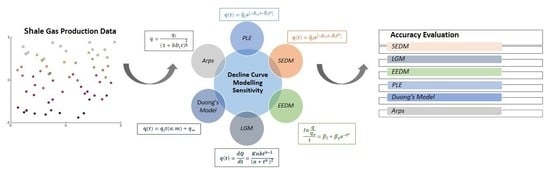
4. Overview of Decline Curve Models

Consistently forecasting the long-term production performance of shale (unconventional) reservoirs has been a challenge [11]. The petroleum industry requires simple, useful, and speedy means of predicting production and assessing reserves; hence, DCA has been an attractive alternative in contrast to other methods [11]. Due to the relative ease of DCA, it is considered the most used method in the industry [11]. The current DCA models will be evaluated based on their characteristics, strengths, weaknesses, and sensitivity to production data.

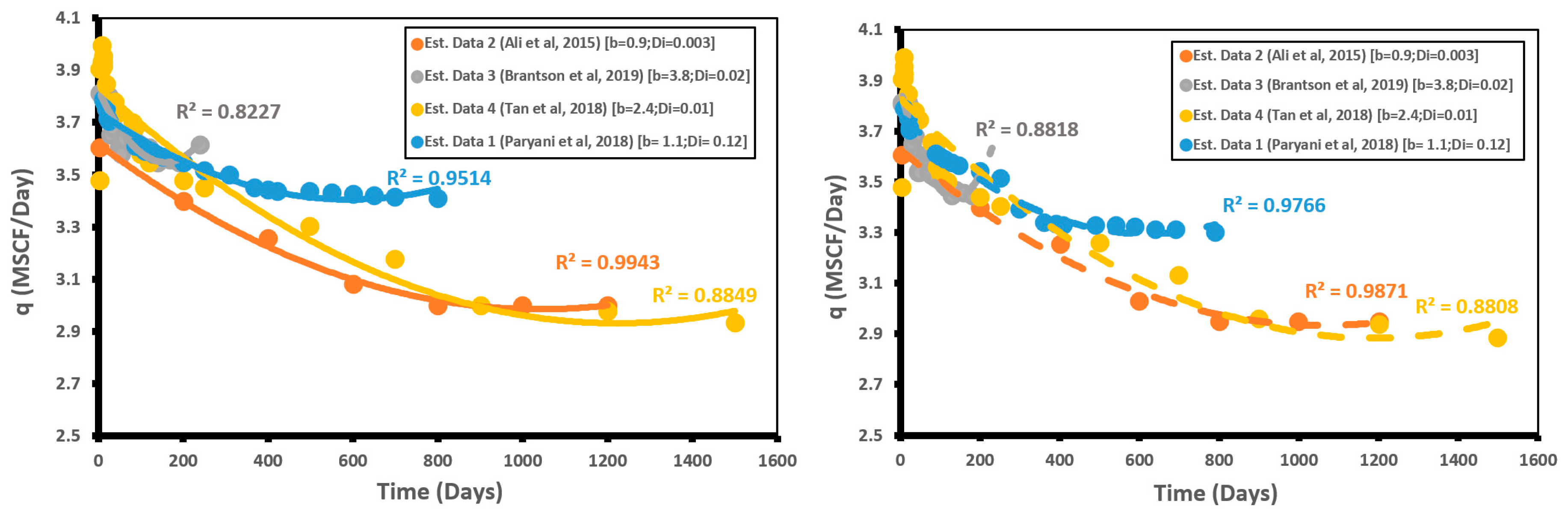
4.1. Arps Decline Curve and the Modified Hyperbolic Decline Model (MHD)

Arps decline curve analysis is the most commonly used method of estimating ultimate recoverable reserves and future performance [12]. Paryani et al. [13] reasons this to reliable history match (even with b > 1) and its simplicity. The model process is based on vital assumptions: that past operating conditions will remain unaffected, a well is produced at or near capacity, and the well’s drainage remains constant and is produced at a constant bottom-hole pressure [14]. Notably, the Arps model is only applicable in pseudo-steady flows when the flow regime transfers from linear flows to boundary-dominated flows (BDF) [15]. This indicates the Arps equations are not applicable to the production forecasting of the entire decline process of horizontal wells in low-permeability reservoirs [16]. The Arps decline curve analysis can be summarised into three types: exponential Equation (1), hyperbolic Equation (2), and harmonic Equation (3) [17,18].

$$q=q_i{e}^{-Dt}$$

(1)

$$q=\frac{q_i}{{\left(1+b{D}_{i}t\right)}^{\frac{1}{b}}}$$

(2)

$$q=\frac{q_i}{1+D_i}$$

(3)

where q is the flow rate in STB/day or Mscf/day, q_i is the initial flow rate in STB/day or Mscf/day, D is the decline constant while D_i is the initial decline constant, which are both measured in days − 1, and b is the decline exponent.

The most commonly employed hyperbolic form of Arps decline Equation (2) is used for shale reservoirs. The hyperbolic decline equation is suitable to use due to the “best fit” that it provides for the long transient linear-flow regime observed in shale gas wells with b values greater than unity [18]. The model results in post-production overestimation due to the decrease in the decline rate with production time. Due to the overestimation, Robertson et al. [19] suggested a revised version of the hyperbolic decline model for shale gas production decline. The equation is given as:

$$q=\frac{q_i}{{\left(1+n{D}_{i}t\right)}^{1/n }} \left(D>D_{lim}\right)$$

(4)

$$q=q_i exp\left(-D_{lim}t\right) \left(D\le D_{lim}\right)$$

(5)

where q is the production rate in m³/d or STB/day, $D_{lim}$ is the decline rate in d⁻¹, and n is the time exponent. They suggested that the hyperbolic decline model sometimes yields unrealistically high reserve estimates. They made an assumption that the rate of decline starts at 30% of flow and usually declines in a hyperbolic way [19]. This modified model considers when the hyperbolic decline in the early life of a well transfers to exponential decline in the late life [19]. The switching process can be determined by applying computer programs. The switching point is when the decline rate is smaller than a certain limit (usually 5%) [19]. The MHD model addresses the overestimation limitation of EUR; however, it is still unable to determine $D_{lim}$ for production data [15].

To test the behavior of the Arps hyperbolic model and the modified version shown in Figure 1, a semi log plot (log q versus t) illustrates the sensitivity of the models to various estimated field data. The R² values denote the goodness of fit or the degree of linear correlation, which is a measure of the level of association of a group of actual observations to the model’s forecasts [20]. As observed from the regression lines for the various data, the resulting fit appears to capture the trend in the data well. Arps fits Data 1 and 2 fairly, similarly for the MHD. However, the methods matches the other cases poorly, because it cannot model multiple flow regimes. In the instance of the MHD model, there is a shift in the curves downward, which results in a change in the R² value. Upon closer inspection of the EUR values for both models, which are shown in

Table 1. Summary of estimated ultimate recovery (EUR). MHD: Modified Hyperbolic Decline Model.

EUR (bscf)	Data 1	Data 2	Data 3	Data 4
Arps Model	0.31	20.52	18.13	5.21
MHD	0.18	4.13	13.18	4.18

, it is evident that the MHD model corrects for the overestimation of the Arps model.

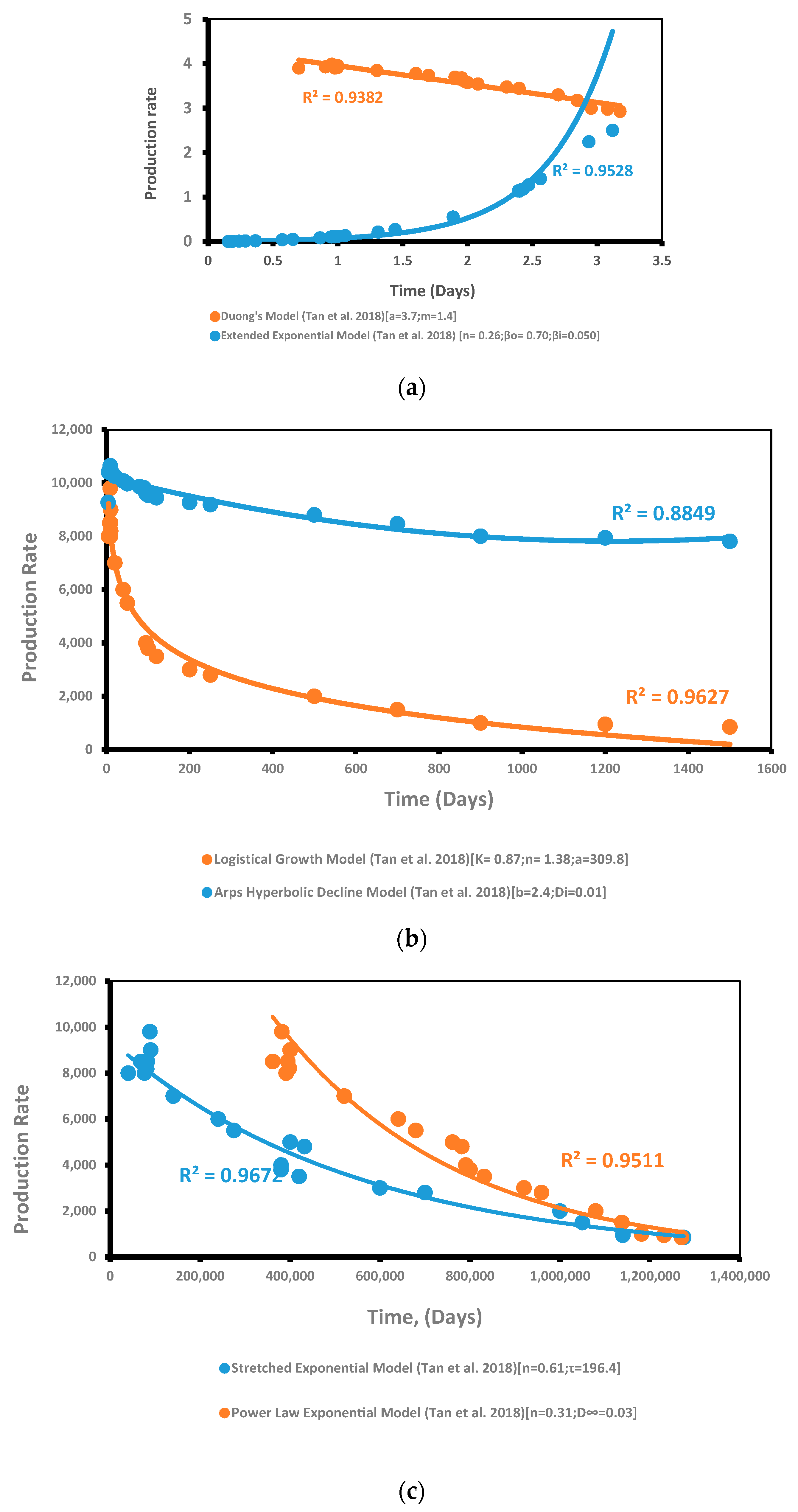
4.2. Power Law Exponential Model (PLE)

Ilk et al. [22] presented the PLE, which is an extension of the exponential Arps formula for the decline degree in shale reservoirs. This model was developed precisely for SGR and approximates the rate of decline with a power law decline. The PLE model matches production data in both the transient and boundary-dominated regions without being hypersensitive to remaining reserve estimates [23]. Seshadri and Mattar [24] presented that the PLE model can model transient radial and linear flows, while Kanfar and Wattenbarger [25] proved that the model is reliable for linear flow, bilinear flow followed by linear flow, and linear flow followed by BDF, or bilinear flow followed by linear flow and finished with BDF flow. Vanorsdale [26] deduced that when the flow regime changes throughout the initial 10 years of the well, the PLE model will yield a very optimistic recovery. The model characterizes the decline rate by infinite time, D∞ which is defined as a “loss ratio” (which is assumed to be constant from Arp) [16]. The production rate is derived as follows:

$$\frac{q}{dq/dt}=-b$$

(6)

$$b=D_{\infty +}{D}_i{t}^{-\left(1-\widehat{n}\right)}$$

(7)

where $dq/dt$ is the slope, D_∞ is the decline rate over a long-term period, and $\widehat{n}$ is the time exponent. By substituting the above equations, the production rate is obtained:

$$q\left(t\right)={\widehat{q}}_i{e}^{\left[-D_{\infty }t-{\widehat{D}}_i{t}^{\widehat{n}}\right]}.$$

(8)

In this model, there are four unknown variables: ${\widehat{q}}_i,{\widehat{D}}_{i,} D_{\infty } and \widehat{n}$, which result in several degrees of freedom and may be clumsy to use or solve [27]. According to Johnson et al. [28], the D∞ parameter is difficult to determine. However, there are advantages to this model in that the extra variables permit for both transient and boundary flow, and the equation for production rate seems comparable to the Arps exponential equation [13]. With the PLE model (Figure 2), which uses a log-log plot (log q versus log t) to test the sensitivity of the data, the resulting fit appears to capture the trend in the data better compared to the Arps Hyperbolic Model. This model fits Data 1, 2, 3, and 4 fairly accurately. This can be attributed to the PLE model, matching production data in both transient and boundary-dominated regions.

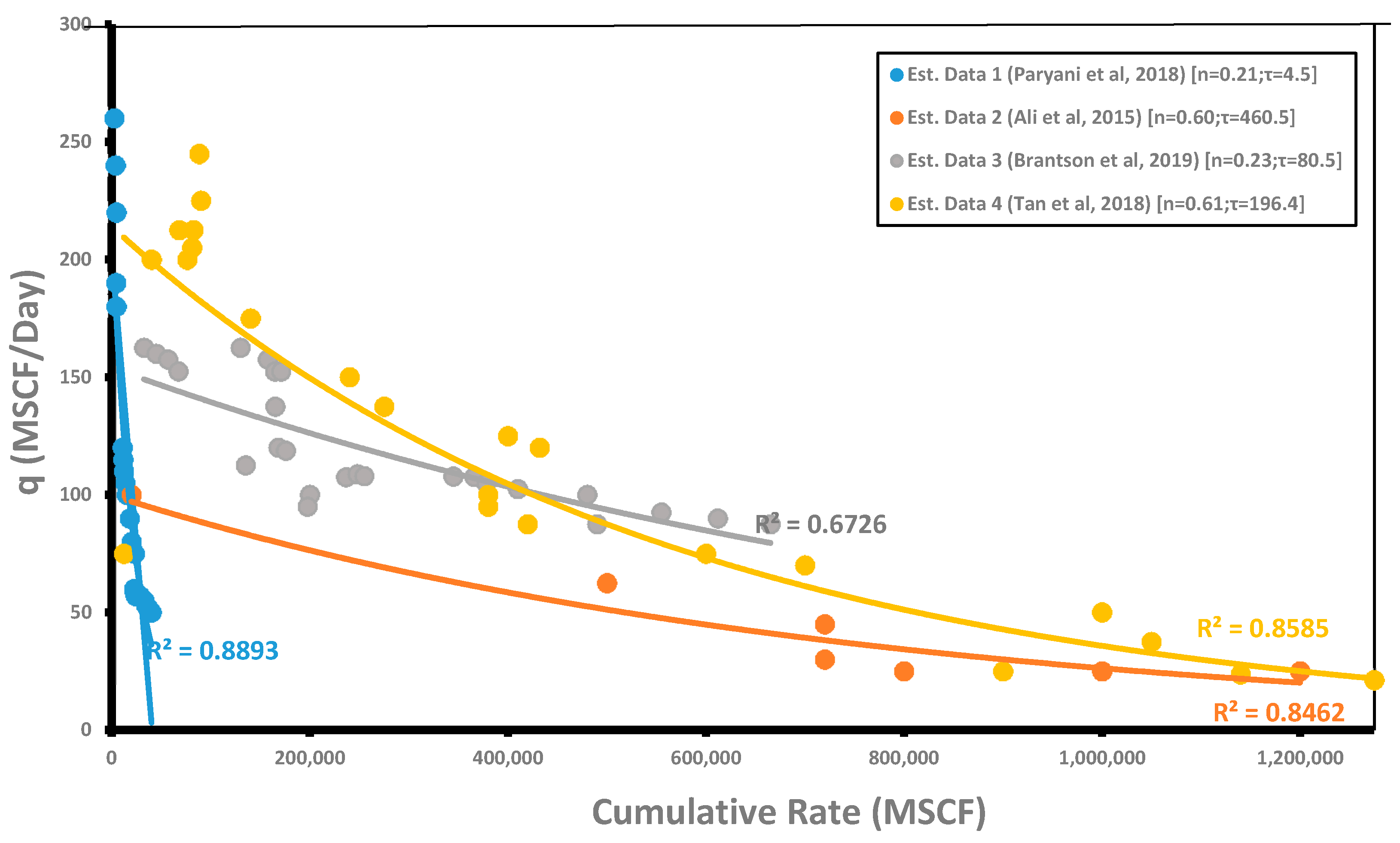
4.3. Stretched Exponential Decline Model (SEDM)

Valkó, Valkó, and Lee [29,30] applied the SEDM in shale wells, which is an empirical method different from Arps equations, as it describes the decline trend of production data obtained from unconventional reservoirs. It was developed to fit transient flow regimes [10,25]. The significant advantages of the model are the bounded nature of estimated ultimate recovery (EUR) without limits on time or rate, and the straight-line behavior of a recovery potential expression [30]. The model differs from other models, since it does have a basis in physics and is directed by a major differential equation [14]. It is used to model aftershock decay rates [31]. The production rate declines with time according to the following equations:

$$\frac{dq}{dt}=-n\left({\frac{t}{\mathsf{\tau }}}^n\right)\frac{q}{t}$$

(9)

$$q=q_{i }\exp \left[-{\left(\frac{t}{\mathsf{\tau }}\right)}^n\right]$$

(10)

$$\mathrm{Ǫ}={\frac{qi}{n}}^n\left\{ɼ\left[\frac{1}{n}\right]-ɼ\left[\frac{1}{n}·{\left(\frac{t}{\mathsf{\tau }}\right)}^n\right]\right\}$$

(11)

$$\mathrm{EUR}={\frac{qi}{n}}^{\mathsf{\tau }}\mathsf{\tau }\left[\frac{1}{n}\right].$$

(12)

This method defines a characteristic number of periods, τ, and a dimensionless exponent, n, of the ratio of time, t. It also uses observed cumulative production along with theoretical cumulative production derived from the integral of the rate-time equation to estimate remaining technically recoverable volumes. Equation (10) appears similar to the PLE model; however, it differs, as it does not rely on a single interpretation of parameters. Instead, it uses two-parameter gamma functions [29]. In addition, there is no single τ and n parameters, but instead, a sum of multiple exponential declines, which follows the fat tail distribution [30]. Stretched Exponential Decline Model (SEDM) requires an iterative process to determine the value of the parameter, n. The model can only estimate the recoverable volumes with an abandonment rate of zero as opposed to commercial volumes with economic cut-off rates and has not been widely used [32]. However, Can et al. [32] showed that in tight formations where transient flow period is extremely long, SEDM has been successful in modeling the rate-time behavior and provides more realistic reserve estimates compared to Arps decline relations.

Testing the behavior of the SEDM, Figure 3, which is a plot of production rate versus the cumulative production (q versus Q) to test the sensitivity of the data, the resulting fit appears to capture the trend in the data poorly. The SEDM method fits all cases inaccurately (lower R² values). This is due to the SEDM model’s transient flow rather than boundary-dominated flow and requirement for a sufficiently long production time (usually >36 months) to accurately estimate the parameters τ and n [33].

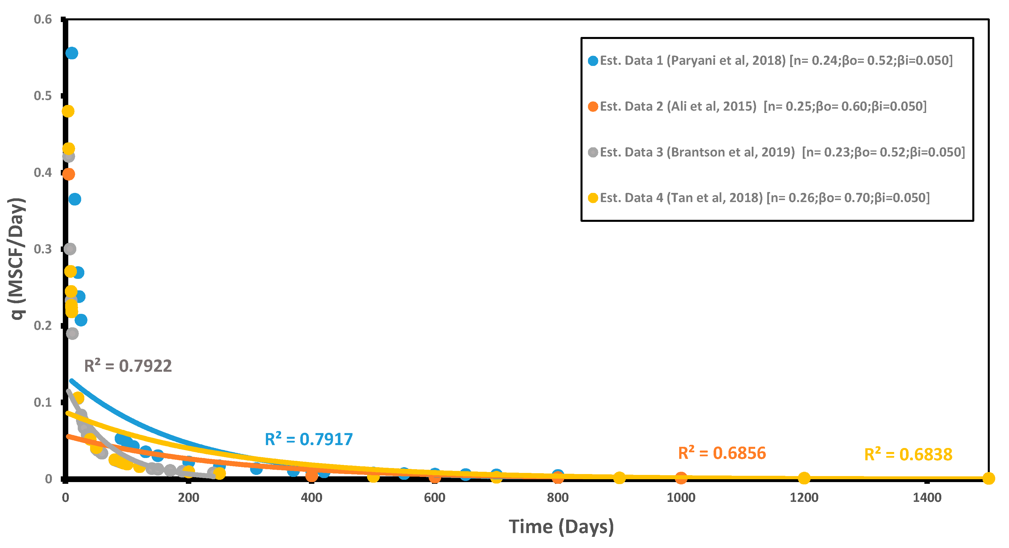
4.4. The Extended Exponential Model (EEDM)

Zang et al. [11] presented a renewed experimental method, the EEDM, as a simple formula to forecast shale oil and gas well performance. They proposed a mechanism of “growing drainage volume” to conceptualize and model the performance of shale wells. This model combines the exponential decline equation proposed by Fetkovich et al. [34] Equation (13) with the derived empirical Equation (14). The EEDM includes both transient and BDF flow in a single equation, and it can match the historical data with a smooth curve throughout the transition period from transient to BDF flow regimes. Furthermore, the model is simple and can easily be applied [11]. It is also able to project the future production by fitting all of the historical production data from the beginning of the production decline.

Paryani et al. [13] stated that the model contains two decline constants and a decline exponent; particularly noteworthy, the production data fits using a smooth curve through the whole flow systems [16]. The advantage of the model is that both early and late production profiles can be captured once ${\beta }_{e }\mathrm{and} {\beta }_l$ have been calibrated using the production data [11]. However, as parameter ${\beta }_l$ has an incomplete influence on the curve fitting, it is therefore fixed.

$$q=q_i{e}^{-at}$$

(13)

$$a={\beta }_l+{\beta }_e$$

(14)

where a is the nominal decline rate, β_l is the late-life period constant, and β_e is the early period constant. Combining Equations (13) and (14) and taking the logarithm of each side, the equation below (the exponential decline equation) is obtained.

$$\frac{In\frac{q}{q_o}}{t}={\beta }_l+{\beta }_e{e}^{-t^n}$$

(15)

where q_o is the initial production rate in m³/s. Using the EEDM (Figure 4), which is a plot of $-ln\frac{q}{qo}/t$ versus t to test the sensitivity of the data, the resulting fit appears to also capture the trend in the data poorly. The method fits all cases inaccurately (lower R² values). This type of method is best to forecast short-term trends in the absence of recurring variations. Hence, the EEDM would only be accurate when a realistic amount of stability between the past and future is assumed.

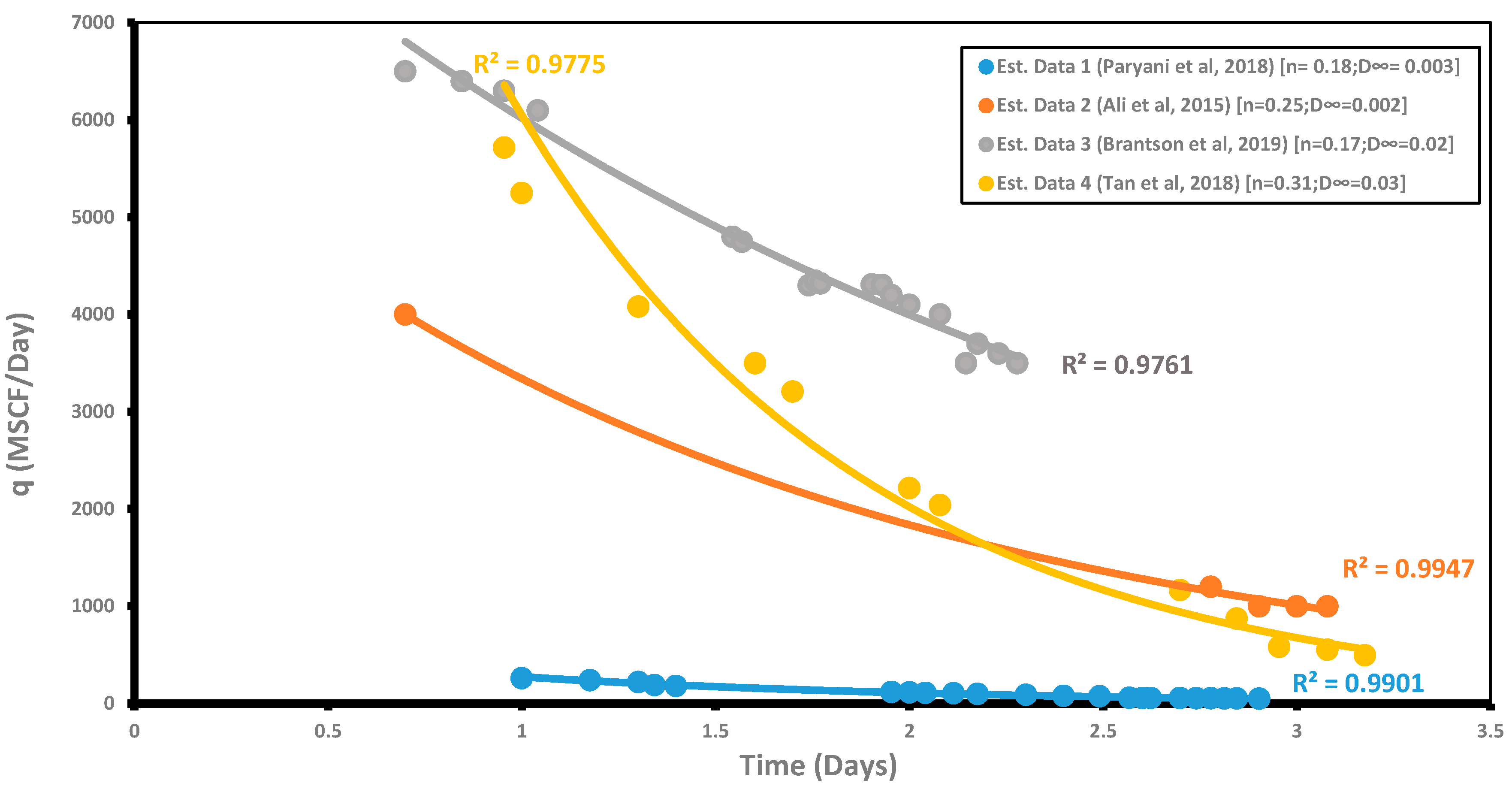
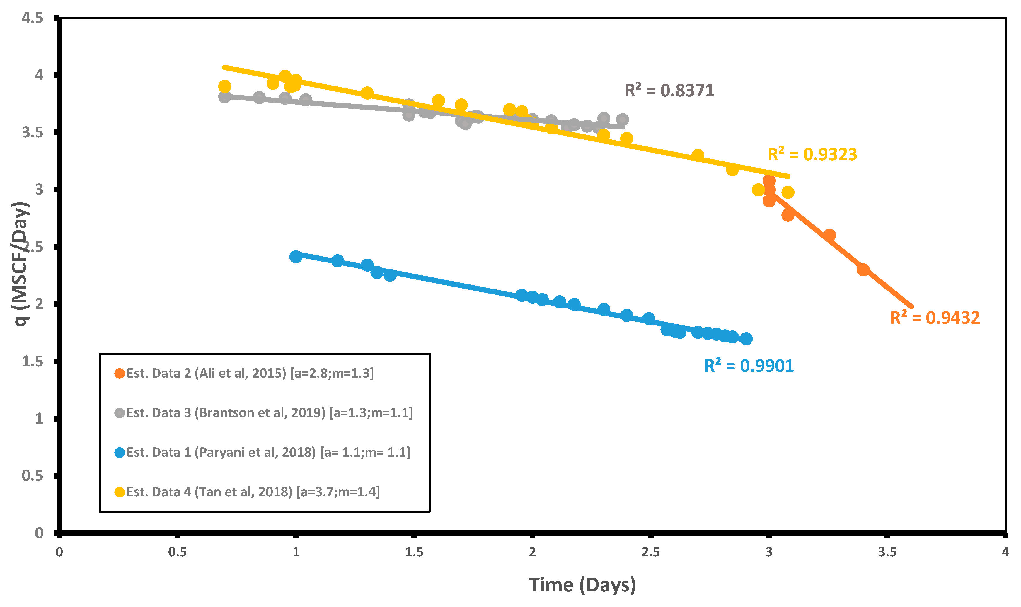
4.5. Doung’s Decline Model

Doung [35] presented an unconventional rate decline method to evaluate the performance of shale gas wells that does not depend on the fracture types. The model assumes linear or near-linear flow, as indicated by a log-log plot of rate over cumulative production versus time, which yielded a straight-line tendency [36]. The rate is calculated in the model using the following equation [27]:

$$q\left(t\right)=q_{i}t\left(a,m\right)+q_{\infty }$$

(16)

where t (a,m) is the time constant in 1/s, and q_∞ is the production rate at infinite time in m³/s. The cumulative production and time constant is calculated as:

$$G_p=\frac{qt\left(a,m\right)}{a{t}^{-m}}$$

(17)

$$t\left(a,m\right)=t^{-m}\exp \left(\frac{a}{1-m}\left(t^{1-m}-1\right)\right)$$

(18)

where G_p is the cumulative gas production in Bcf and m is the slope.

Paryani et al. [13] indicated the key restrictions of the model: if the well is closed for extended periods, a proper rate initialization against pressure is required to obtain precise values of parameters a and m and, secondly, that in the event of water breakthrough, there is a sudden decrease in the decline rate, and this causes an increase in the values of the a and m parameters. Vanorsdale [26], similar to in the case of the PLE model, also indicated that the Doung model will yield a very optimistic recovery when the flow regime changes throughout the initial 10 years. He went on to indicate that the model may provide conservative recovery estimate in vertical, non-hydraulic fractured classical shale wells [26]. However, Lee et al. [36] has indicated that the Doung’s model appears to fit field data from various shale plays quite well and provides an effective alternative to Arps hyperbolic model. With the Duong’s model (Figure 5), which uses a log-log linear plot (log q versus log t) to test the sensitivity of the data, the resulting fit appears to capture the trend in the data well. The method fits Data 1, 2, and 4 fairly accurately. For Case 3, the method fits the data poorly with a lower R² value of 0.8371. The model probably provides a good fit because it was specifically developed for unconventional reservoirs with very low permeability.

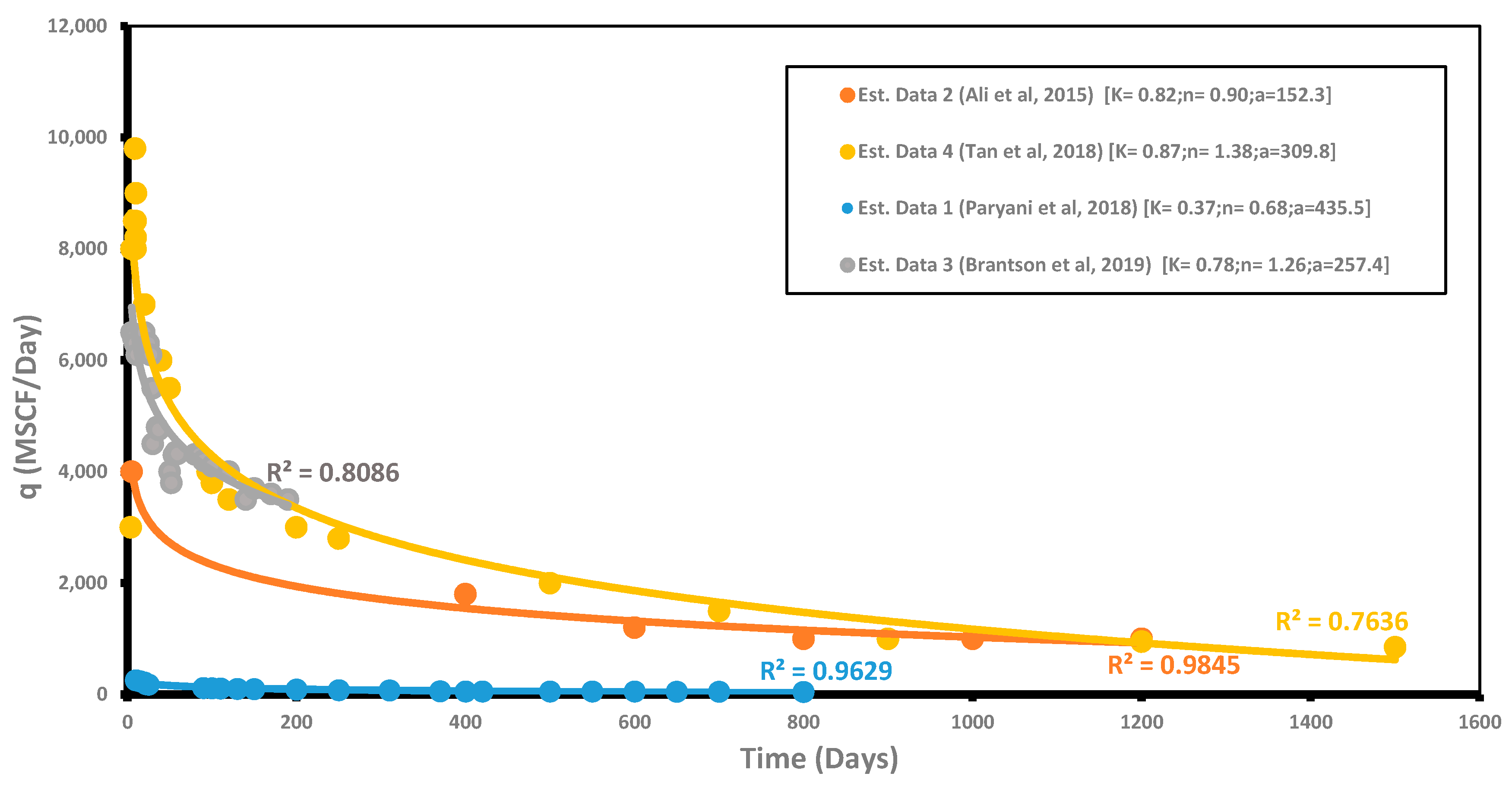
4.6. Logistic Growth Model (LGM)

Logistic Growth Models developed belong to a group of mathematical models used to forecast growth in numerous applications [36] and were previously used to model population growth [37,38]. It was developed to forecast reservoirs with extremely low permeability [27]. LGM is very flexible and confident in modelling long transient boundary-dominated performances of unconventional reservoirs [16]. The model incorporates known physical volumetric quantities of oil and gas into the forecast to constrain the reserve estimate to a reasonable quantity. LGM is capable of trending existing production data and providing reasonable forecasts of future production. The logistic growth model does not extrapolate to non-physical values [38]. Tsoularis and Wallace [39] discussed a development in this regard by Verhulst [40], who considered that for the population model, a steady population would consequently possess a saturation level characteristic, typically called the carrying capacity, K, which forms a numerical upper bound on the growth size. In order to include this limiting characteristic, they introduced the logistic growth equation as an extension to the exponential model [39]. Zhang et al. [1] adopted this model for SGR with very low permeability and developed the LGM as an empirical method to forecast the gas production. The LGM can be represented as follows:

$$q\left(t\right)=\frac{dQ}{dt}=\frac{Knb{t}^{n-1}}{{\left(a+t^{n }\right)}^2}$$

(19)

where K is the carrying capacity.

The main benefit of the LGM is that the reserve estimate is inhibited by the parameter K as well as the production rate, which terminates at infinite time [1]. The main assumption in this model is that the whole reservoir can be drained by a single well over a suitably long period and requires the approximation of at least two parameters, or parameters as per the available well information [4,7]. Figure 6, a plot of production rate versus time (q versus t), illustrates the sensitivity of the model to various estimated field data. As observed from the regression lines for the various data, the resulting fit appears to capture the trend in the data well. The LGM fits Data 1 and 2 fairly. However, the method matches the other cases poorly, as indicated by the lower R² values. This could be attributed to the data size, which is too small to yield an accurate fit, since the underlying principle of this model is population growth, which stipulates that growth is only possible up to a certain size.

4.7. Autoregressive Intergrated Moving Average (ARIMA) and Neutral Network Models (NNM) (Hybrid Model)

The accuracy of time series forecasting is challenging for scientists [41]. Time series data often comprise linear as well as non-linear components [42]. In some cases, linear-based approaches might be more suitable than non-linear ones due to the data characteristics. The hybrid method is a combination of ARIMA and the neural network method. According to Faruk [42], hybrid methods have a higher degree of accuracy than neural networks. ARIMA can recognize time-series patterns well but not non-linear data patterns. On the other hand, neural networks only handle non-linear data. Therefore, hybrid models combine the advantages of ARIMA with respect to linear modelling and neural networks in terms of non-linear edge modelling [43]. Notwithstanding, in some circumstances, the single model approach can outperform hybrid models [41].

Mathematically, time-series data can be expressed as a combination of linear and non-linear components [44]:

$$Y_t=L_t+N_t$$

(20)

where Y_t shows the time-series data, L_t indicates the linear components, and the non-linear components are represented by N_t.

Mathematically, the neural network model for residual of n input nodes can be expressed as the following:

$$e_t=f\left(e_{t-1}+e_{t-2},\dots ,e_{t-n}\right)$$

(21)

where f is a non-linear function that is specified by the neural network. With regard to the results of the prediction error of N_t, the combination forecast using the hybrid method can be expressed as:

$${\widehat{y}}_t={\widehat{L}}_t+{\widehat{N}}_t$$

(22)

There has been limited work conducted using this model for shale gas reservoirs. Hence, the next step would be to investigate this model for shale gas reservoirs.

To summarize all eight DCA models for an easy reference of readers,

Table 2. Summary of decline curve analysis (DCA) models. BDF: boundary-dominated flows, SGR: shale gas reservoirs.

No	Model	Equation	Production Behaviour	Strength	Weakness	Reference
1	Arps Hyperbolic Decline	$q=\frac{q_i}{{\left(1+b{D}_{i}t\right)}^{\frac{1}{b}}}$	linear to BDF flow	reliable and simple to use	post-production overestimation	[12,13,14,15,16,17,18]
2	Modified Hyperbolic Curve	$\begin{array}{l}q\\ =\frac{q_i}{{\left(1+n{D}_{i}t\right)}^{1/n}} \left(D>D_{lim}\right)\end{array}$ $\begin{array}{l}q\\ =q_i exp\left(-D_{lim}t\right) \left(D\le D_{lim}\right)\end{array}$	transient and BDF flow	addresses the overestimation limitation of EUR	still unable to determine $D_{lim}$ for production data	[15,19]
3	Power Law Exponential Decline	$q\left(t\right)={\widehat{q}}_i{e}^{\left[-D_{\infty }t-{\widehat{D}}_i{t}^{\widehat{n}}\right]}$	transient and BDF flow	developed precisely for SGR	four unknown variables to solve	[13,16,20,23,24,25,26,27]
4	Stretched Exponential Decline	$q=q_{i }exp\left[-{\left(\frac{t}{\tau }\right)}^n\right]$	transient flow	bounded nature of EUR and straight-line behavior of recovery potential expression	requires sufficiently long production times	[10,14,26,28,29,30,31,32]
5	The Extended Exponential Model	$\frac{\mathrm{In}\frac{q}{q_o}}{t}={\beta }_{\mathrm{l}}+{\beta }_e{e}^{-t^n}$	transient and BDF flow	both early and late production profiles can be captured	parameter ${\beta }_l$ has an incomplete influence on the curve fitting and is therefore fixed	[11,13,16,33]
6	Doung’s Decline	$\begin{array}{l}t\left(a,m\right)\\ =t^{-m}exp\left(\frac{a}{1-m}\left(t^{1-m}-1\right)\right)\end{array}$	linear or near-linear flow	appears to fit field data from various shale plays	extended periods, a proper rate initialization against pressure is required, and in the event of water breakthrough, a and m increases	[13,20,27,34,35]
7	Logistic Growth	$q\left(t\right)=\frac{dQ}{dt}=\frac{Knb{t}^{n-1}}{{\left(a+t^{n }\right)}^2}$	long transient boundary-dominated	reserve estimate is inhibited by K as well as the production rate, which terminates at infinite time	growth is only possible up to a certain size	[1,16,20,35,36,37,38,39]
8	Hybrid Model	$\varnothing \left(B\right){(1-B)}^d{Y}_t=\theta \left(B\right){\epsilon }_t$	linear and non-linear	high degree of accuracy	approach can be found to not be fit all types of data	[40,41,42,43]

lists the name of each model, its DCA equation, the characteristic, strength, weakness, and lastly the related references.

5. Accuracy of Current Decline Curve Models with Field Data

Yuhu et al. [15] discussed comparisons of EURs with five types of decline models from single-well production data. They explained that according to the prediction results, the highest predicted EUR was gained by the hyperbolic decline model, followed by the Modified Hyperbolic Model (MHD), Doung’s Model, PLE and, lastly, the EDM. Hu et al. [27] conferred production data for wells with a production time greater than 10 years, for which the PLE decline model was recommended for multiple flows. It was also pointed out that the hyperbolic decline model predicted higher estimates of reserves than the PLE decline model. Another study that they reviewed recommended the MHD rather than the PLE decline model, which in their view was complicated.

It is noted that the differences in EURs with different decline models decrease with an increase in production time [45]. On the other hand, prediction consistency increases with an increase in production time. Based on this distinctive production data, the order of predicted EURs from high to low were through the hyperbolic decline model, the MHD, the PLE decline model, and the EDM respectively [45]. The predicted EURs decreased with an increase of production time for the hyperbolic decline and the modified hyperbolic decline model. The predicted EURs increase with an increase of production time for the PLE decline and the EDM model [45]. Currently, the applicability of these different decline models is uncertain. The general trend found in their paper was that the hyperbolic decline model overestimates the production and that the other decline models will still have to be investigated for reliability and accuracy [45].

In their study, Guo et al. [46] investigated shale gas wells in the Barnett shale play, where they found that from the results of goodness of fit, the hyperbolic curve fits well for both the aggregate and individual shale gas wells. On the other hand, Kenomore et al. [47] in their production decline study of the Barnett shale found that either the Arps hyperbolic or Doung’s model can be used only if the historical data exceeds 10 months. They used root mean square error (RMSE) analysis and the results indicated that the Arps hyperbolic model showed better forecasting compared to the Doung’s model for the top three longest production histories. Zhang et al. [1] concurred with the findings of the Doung’s model in their paper, noting that it is more accurate for linear flow and bilinear flow; however, if the production history is shorter than 18 months, this model provides unreliable results for EUR. In most circumstances, the Doung’s model overestimates the total EUR. Harris [48], in his research study of the Elm Coulee field production data, found that the Duong method will produce the most optimistic forecasts followed by the Arps model with 5% minimum decline, and then the SEPD model. Shah [49] in his research developed new methods of combining the SEPD and Arps hyperbolic equation, the Doung’s with the Arps hyperbolic equation, and the Arps super hyperbolic combined with the Arps hyperbolic decline equation. He found that the SEPD and Arps hyperbolic equation gave the most conservative results of all the methods in the study, even if there was insufficient data available. This equation can also work without enough boundary-dominated flow (BDF) data available.

Hu et al. [27] studied DCA techniques for the Eagle Ford and Austin Chalk reservoirs. They found that in the case of the Eagle Ford reservoir, the MHD and the Doung’s model provided the highest EUR estimations and the two lowest matching errors, while the PLE decline model with $D_{\infty }\ne 0$ produced the lowest EUR estimates with the highest matching errors in all cases. In another study, according to the results of goodness of fit (R² and N-RMSE), the hyperbolic model fits well with aggregated well data and with individual wells [1]. Further, in their study, Hu et al. [27] explain that the LGM and PLE model with $D_{\infty }=0$ gave production projections neither too positive nor too traditional with modest matching errors. Therefore, they recommend both the MHD and Doung’s model for this reservoir. However, Zhang et al. [11] developed the EEDM and verified their model using field data from the Eagle Ford. They found this model to be more rigorous in that it will include the effects of interference among adjacent fractures, variable permeability, and discontinuous pressure distribution, which are difficult to capture and model with other DCA methods [11]. In the case of the Austin Chalk reservoirs, all DCA methods resulted in fairly similar EUR forecasts and matching errors; hence, any method can be used [27]. Figure 7, which uses estimated production data versus time values, indicates that using the R² values as a goodness of fit to determine the accuracy of the different decline models, the SEDM, followed by the LGM, EEDM, PLE, Doung’s decline model and, lastly, the hyperbolic decline model would predict the EUR accurately.

During their case study analysis, Paryani et al. [13] found that the LGM, PLE, and Doung’s models overcame Arps limitations to a certain degree. The PLE model always predicted the lowest forecasts of all the models with the most conservative production forecasting and reserve estimation. Doung’s model performed the best for longer when less noisy production data was available; however, erratic EUR was observed, which indicates that this model requires further improvements [13]. The LGM gave reasonable EUR estimates when compared to the Arps model. There was an 81% fit of the wells’ past production rate and cumulative production. The LGM also appears most effective at historically matching past production and predicting finite reasonable EUR. However, Tan et al. [4] found that due to the constraints of K and the vanishing production rate at infinity time, the LGM provides a finite estimate of EUR. They also determined by using normalized and logarithmic rate-time residuals that the limitations of the Arps model are overcome and accuracy improves in cases of unconventional reservoirs.

6. Conclusions

Shale gas reservoirs have become an essential source for providing natural gas globally and the process of hydraulic fracking has been used in the extraction of shale gas. During the fracking process, there are different flow regimes, which occur during the life cycle of SGRs, these being fracture linear flow, fracture boundary flow, matrix linear flow, and matrix boundary flow. They are significant because they impact both the production and decline behavior of SGRs.

Based on previous studies conducted, it was found that the Arps hyperbolic decline, the MHD and Doung’s models provided the best fit with production data. However, contrary to the reviewed studies when estimated production data was used in the evaluation process for the basis of this paper, using the goodness-of-fit technique, the PLE and Doung’s decline models aligned the best with the production data compared to the other models.

It is evident from the accuracy assessment decline curve modelling impacts the EUR of SGRs, and it was observed that all decline models yield a different EUR result, which is either over or underestimated. Studies have revealed that the production time significantly impacts the EUR depending on which decline model is being used. When each model was assessed for accuracy once again using the goodness-of-fit technique, the results indicated the SEDM, followed by the LGM, EEDM, PLE, Doung’s decline model and, lastly, the hyperbolic decline model align with the production data.

It is evident from the decline curve evaluation there are advantages in using the current DCA models; however, they also have limitations associated with them, which have to be addressed. Therefore, the next step will be to evaluate the use of the hybrid model in evaluating the decline of SGR.

References

1. Zhang, X.; Wang, X.; Hou, X.; Xu, W. Rate decline analysis of vertically fractured wells in shale gas reservoirs. Energies 2017, 10, 1602. [Google Scholar] [CrossRef] [Green Version]
2. Wang, H. What factors control shale gas production and production decline trend in fractured systems: A comprehensive analysis and investigation. SPE J. 2017, 22, 562–581. [Google Scholar] [CrossRef] [Green Version]
3. Xu, B.; Haghighi, M.; Li, X.; Cooke, D. Development of new type curves for production analysis in naturally fractured shale gas/tight gas reservoirs. J. Pet. Sci. Eng. 2013, 105, 107–115. [Google Scholar] [CrossRef]
4. Tan, L.; Zuo, L.; Wang, B. Methods of decline curve analysis for shale gas reservoirs. Energies 2018, 11, 552. [Google Scholar] [CrossRef] [Green Version]
5. Yuan, J.; Luo, D.; Feng, L. A review of the technical and economic evaluation techniques for shale gas development. Appl. Energy 2015, 148, 49–65. [Google Scholar] [CrossRef]
6. Knudsen, B.R.; Foss, B.; Whitson, C.H.; Conn, A.R. Target-rate tracking for shale-gas multi-well pads by scheduled shut-ins. IFAC Proc. Vol. 2012, 45, 107–113. [Google Scholar] [CrossRef] [Green Version]
7. Nwaobi, U.; Anandarajah, G.A. Critical Review of Shale Gas Production Analysis and Forecast Methods. Saudi J. Eng. Technol. (SJEAT) 2018, 3, 276–285. [Google Scholar]
8. Adekoya, F. Production Decline Analysis of Horizontal Well in Gas Shale Reservoirs. Master’s Thesis, West Virginia University, Morgantown, WV, USA, 2009. [Google Scholar]
9. Nelson, P.H. Pore-throat sizes in sandstones, tight sandstones, and shales. AAPG Bull. 2009, 93, 329–340. [Google Scholar] [CrossRef]
10. Joshi, K.J. Comparison of Various Deterministic Forecasting Techniques in Shale Gas Reservoirs with Emphasis on the Duong Method. Ph.D. Thesis, Texas A&M University, College Station, TX, USA, 2012. [Google Scholar]
11. Zhang, H.; Rietz, D.; Cagle, A.; Cocco, M.; Lee, J. Extended exponential decline curve analysis. J. Nat. Gas Sci. Eng. 2016, 36, 402–413. [Google Scholar] [CrossRef]
12. Boah, E.A.; Borsah, A.A.; Brantson, E.T. Decline Curve Analysis and Production Forecast Studies for Oil Well Performance Prediction: A Case Study of Reservoir X. Int. J. Eng. Sci. (IJES) 2018, 7, 56–67. [Google Scholar]
13. Paryani, M.; Ahmadi, M.; Awoleke, O.; Hanks, C. Decline Curve Analysis: A Comparative Study of Proposed Models Using Improved Residual Functions. J. Pet. Environ. Biotechnol. 2018, 9, 362. [Google Scholar]
14. Ali, T.A.; Sheng, J.J. Production decline models: A comparison study. In Proceedings of the SPE Eastern Regional Meeting, Morgantown, WV, USA, 13–15 October 2015. [Google Scholar]
15. Yuhu, B.; Guihua, C.; Bingxiang, X.; Ruyong, F.; Ling, C. Comparison of typical curve models for shale gas production decline prediction. China Pet. Explor. 2016, 21, 96–102. [Google Scholar]
16. Li, P.; Hao, M.; Hu, J.; Ru, Z.; Li, Z. A new production decline model for horizontal wells in low-permeability reservoirs. J. Pet. Sci. Eng. 2018, 171, 340–352. [Google Scholar] [CrossRef]
17. Arps, J.J. Analysis of decline curves. Trans. AIME 1945, 160, 228–247. [Google Scholar] [CrossRef]
18. Qu, Z.; Lin, J.E. (Eds.) Proceedings of the International Field Exploration and Development Conference 2017; Springer: Singapore, 2018. [Google Scholar]
19. Robertson, S. Generalised Hyperbolic Equation; Society of Petroleum Engineers: Richardson, TX, USA, 1988. [Google Scholar]
20. Bagozzi, R.P.; Yi, Y. On the evaluation of structural equation models. J. Acad. Mark. Sci. 1988, 16, 74–94. [Google Scholar] [CrossRef]
21. Brantson, E.T.; Ju, B.; Ziggah, Y.Y.; Akwensi, P.H.; Sun, Y.; Wu, D.; Addo, B.J. Forecasting of Horizontal Gas Well Production Decline in Unconventional Reservoirs using Productivity, Soft Computing and Swarm Intelligence Models. Nat. Resour. Res. 2019, 28, 717–756. [Google Scholar] [CrossRef]
22. Ilk, D.; Rushing, J.A.; Perego, A.D.; Blasingame, T.A. Exponential vs hyperbolic decline in tight gas sands: Understanding the origin and implications for reserve estimates using Arps decline curves. In Proceedings of the SPE Annual Technical Conference and Exhibition, Denver, CO, USA, 21–24 September 2008. [Google Scholar]
23. McNeil, R.; Jeje, O.; Renaud, A. Application of the power law loss-ratio method of decline analysis. In Proceedings of the Canadian International Petroleum Conference, Calgary, AB, Canada, 16–18 June 2009. [Google Scholar]
24. Seshadri, J.N.; Mattar, L. Comparison of power law and modified hyperbolic decline methods. In Proceedings of the Canadian Unconventional Resources and International Petroleum Conference, Calgary, AB, Canada, 19–21 October 2010. [Google Scholar]
25. Kanfar, M.S.; Wattenbarger, R.A. Comparison of Empirical Decline Curve Methods for Shale Wells. In Proceedings of the SPE Canadian Unconventional Resources Conferences, Calgary, AB, Canada, 30 October–1 November 2012. [Google Scholar]
26. Vanorsdale, C.R. Production decline analysis lessons from classic shale gas wells. In Proceedings of the SPE Annual Technical Conference and Exhibition, New Orleans, LA, USA, 30 September–2 October 2013. [Google Scholar]
27. Hu, Y.; Weijermars, R.; Zuo, L.; Yu, W. Benchmarking EUR estimates for hydraulically fractured wells with and without fracture hits using various DCA methods. J. Pet. Sci. Eng. 2018, 162, 617–632. [Google Scholar] [CrossRef]
28. Johnson, N.L.; Currie, S.M.; Ilk, D.; Blasingame, T.A. A Simple methodology for direct estimation of gas-in-place and reserves using rate-time data. In Proceedings of the SPE Rocky Mountain Petroleum Technology Conference, Denver, CO, USA, 14–16 April 2009. [Google Scholar]
29. Valko, P.P. Assigning value to stimulation in the Barnett Shale: A simultaneous analysis of 7000 plus production hystories and well completion records. In Proceedings of the SPE Hydraulic Fracturing Technology Conference, The Woodlands, TX, USA, 19–21 January 2009. [Google Scholar]
30. Valkó, P.P.; Lee, W.J. A better way to forecast production from unconventional gas wells. In Proceedings of the SPE Annual Technical Conference and Exhibition, Florence, Italy, 19–22 September 2010. [Google Scholar]
31. Kisslinger, C. The stretched exponential function as an alternative model for aftershock decay rate. J. Geophys. Res.: Solid Earth 1993, 98, 1913–1921. [Google Scholar] [CrossRef]
32. Can, B.; Kabir, C.S. Probabilistic performance forecasting for unconventional reservoirs with stretched-exponential model. In Proceedings of the North American Unconventional Gas Conference and Exhibition, The Woodlands, TX, USA, 14–16 June 2011. [Google Scholar]
33. Zhou, L.Z.; Selim, H.M. Application of the fractional advection-dispersion equation in porous media. Soil Sci. Soc. Am. J. 2003, 67, 1079–1084. [Google Scholar] [CrossRef]
34. Fetkovich, M.J. Decline curve analysis using type curves. J. Pet. Technol. 1980, 32, 1065–1077. [Google Scholar] [CrossRef]
35. Duong, A.N. Rate-decline analysis for fracture-dominated shale reservoirs. SPE Reserv. Eval. Eng. 2011, 14, 377–387. [Google Scholar] [CrossRef] [Green Version]
36. Lee, K.S.; Kim, T.H. Integrative Understanding of Shale Gas Reservoirs; Springer: Heidelberg, Germany, 2016. [Google Scholar]
37. Clark, A.J. Decline Curve Analysis in Unconventional Resource Plays Using Logistic Growth Models. Ph.D. Thesis, The University of Texas at Austin, Austin, TX, USA, 2011. [Google Scholar]
38. Clark, A.J.; Lake, L.W.; Patzek, T.W. Production forecasting with logistic growth models. In Proceedings of the SPE Annual Technical Conference and Exhibition, Denver, CO, USA, 30 October–2 November 2011. [Google Scholar]
39. Tsoularis, A.; Wallace, J. Analysis of logistic growth models. Math. Biosci. 2002, 179, 21–55. [Google Scholar] [CrossRef] [Green Version]
40. Bacaër, N. Verhulst and the logistic equation (1838). In A Short History of Mathematical Population Dynamics; Springer: London, UK, 2011; pp. 35–39. [Google Scholar]
41. Taskaya-Temizel, T.; Ahmad, K. Are ARIMA neural network hybrids better than single models? In Proceedings of the International Joint Conference on Neural Networks (IJCNN 2005), Montr’eal, QC, Canada, 31 July–4 August 2005. [Google Scholar]
42. Faruk, D.Ö. A Hybrid Neural Network and ARIMA Model for Water Quality Time Series Prediction. Eng. Appl. Artif. Intell. 2010, 23, 586–594. [Google Scholar] [CrossRef]
43. Cybenko, G. Approximation by Superpositions of a Sigmoidal Function. Math. Control Signals Syst. 1989, 2, 303–314. [Google Scholar] [CrossRef]
44. Dhini, A.; Riefqi, M.; Puspasari, M.A. Forecasting analysis of consumer goods demand using neural networks and ARIMA. Int. J. Technol. 2015, 6, 872–880. [Google Scholar] [CrossRef]
45. Wachtmeister, H.; Lund, L.; Aleklett, K.; Höök, M. Production decline curves of tight oil wells in eagle ford shale. Nat. Resour. Res. 2017, 26, 365–377. [Google Scholar] [CrossRef] [Green Version]
46. Guo, K.; Zhang, B.; Wachtmeister, H.; Aleklett, K.; Höök, M. Characteristic Production Decline Patterns for Shale Gas Wells in Barnett. Int. J. Sustain. Future Hum. Secur. 2017, 5, 11–20. [Google Scholar] [CrossRef]
47. Kenomore, M.; Hassan, M.; Malakooti, R.; Dhakal, H.; Shah, A. Shale gas production decline trend over time in the Barnett Shale. J. Pet. Sci. Eng. 2018, 165, 691–710. [Google Scholar] [CrossRef] [Green Version]
48. Harris, S.C. A Study of Decline Curve Analysis in the Elm Coulee Field. Ph.D. Thesis, Texas A&M University, College Station, TX, USA, 2013. [Google Scholar]
49. Shah, S. Development of New Decline Model for Shale Oil Reserves. Ph.D. Thesis, University of Houston, Houston, TX, USA, 2013. [Google Scholar]
Figure 1. Data sensitivity using the Arps Hyperbolic Decline Model [4,13,14,21].
Energies 13 02765 g001
Figure 2. Data sensitivity using the Power Law Exponential Model [4,13,14,21].
Energies 13 02765 g002
Figure 3. Data sensitivity using the Stretched Exponential Decline Model [4,13,14,21].
Energies 13 02765 g003
Figure 4. Data sensitivity using the Extended Exponential Model [4,13,14,21].
Energies 13 02765 g004
Figure 5. Data sensitivity using Doung’s Decline Model [4,13,14,21].
Energies 13 02765 g005
Figure 6. Data sensitivity using the Logistic Growth Model [4,13,14,21].
Energies 13 02765 g006
Figure 7. Estimated production data to determine goodness of fit for accuracy of the different decline models (a) Duong’s Model vs EEDM; (b) LGM vs Arps Hyperbolic Model and (c) SEDM vs PLE [4].
Energies 13 02765 g007