Decoupling Economic Growth from Fossil Fuel Use—Evidence from 141 Countries in the 25-Year Perspective


Abstract
1. Introduction
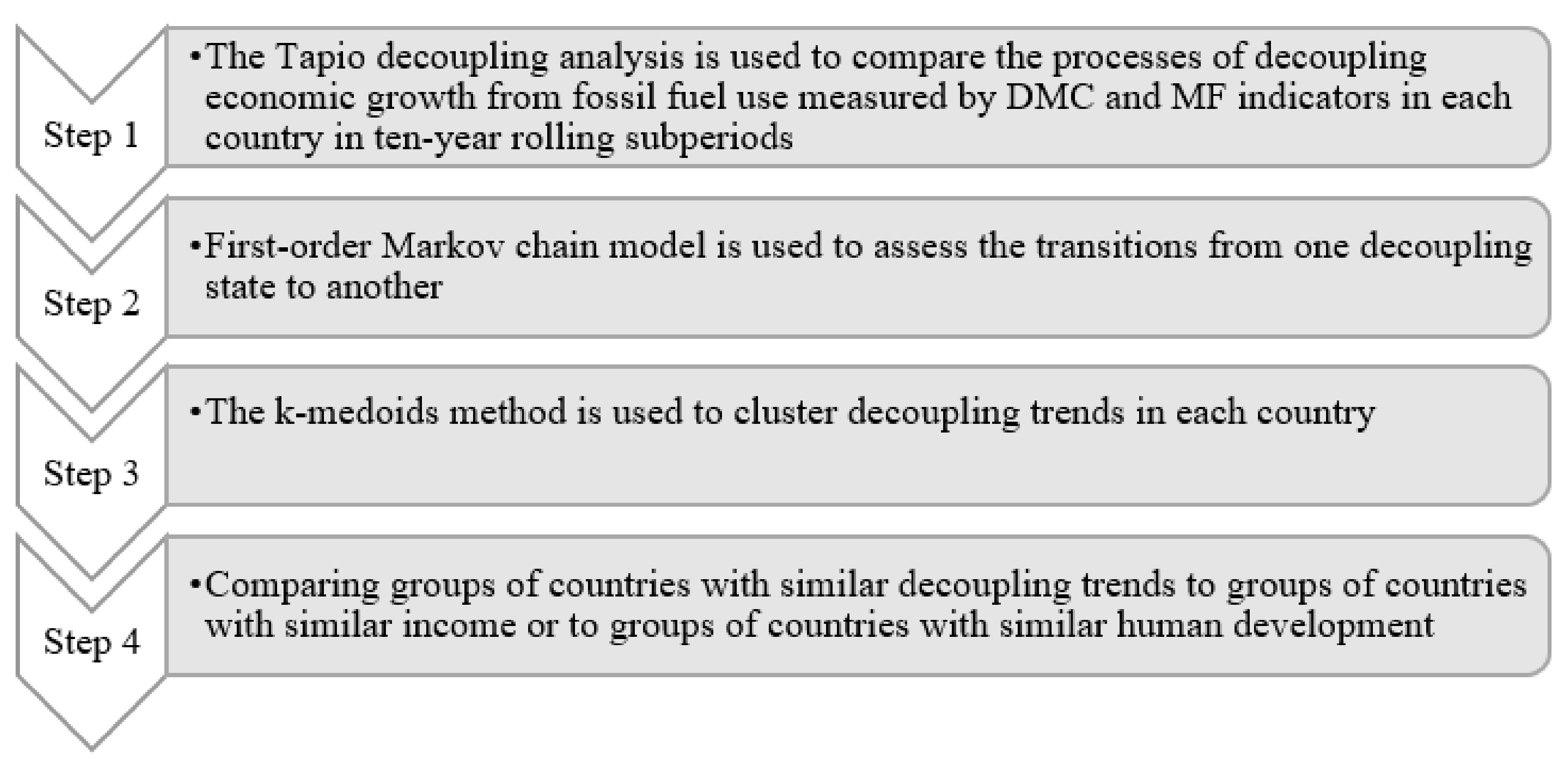
2. Materials and Methods
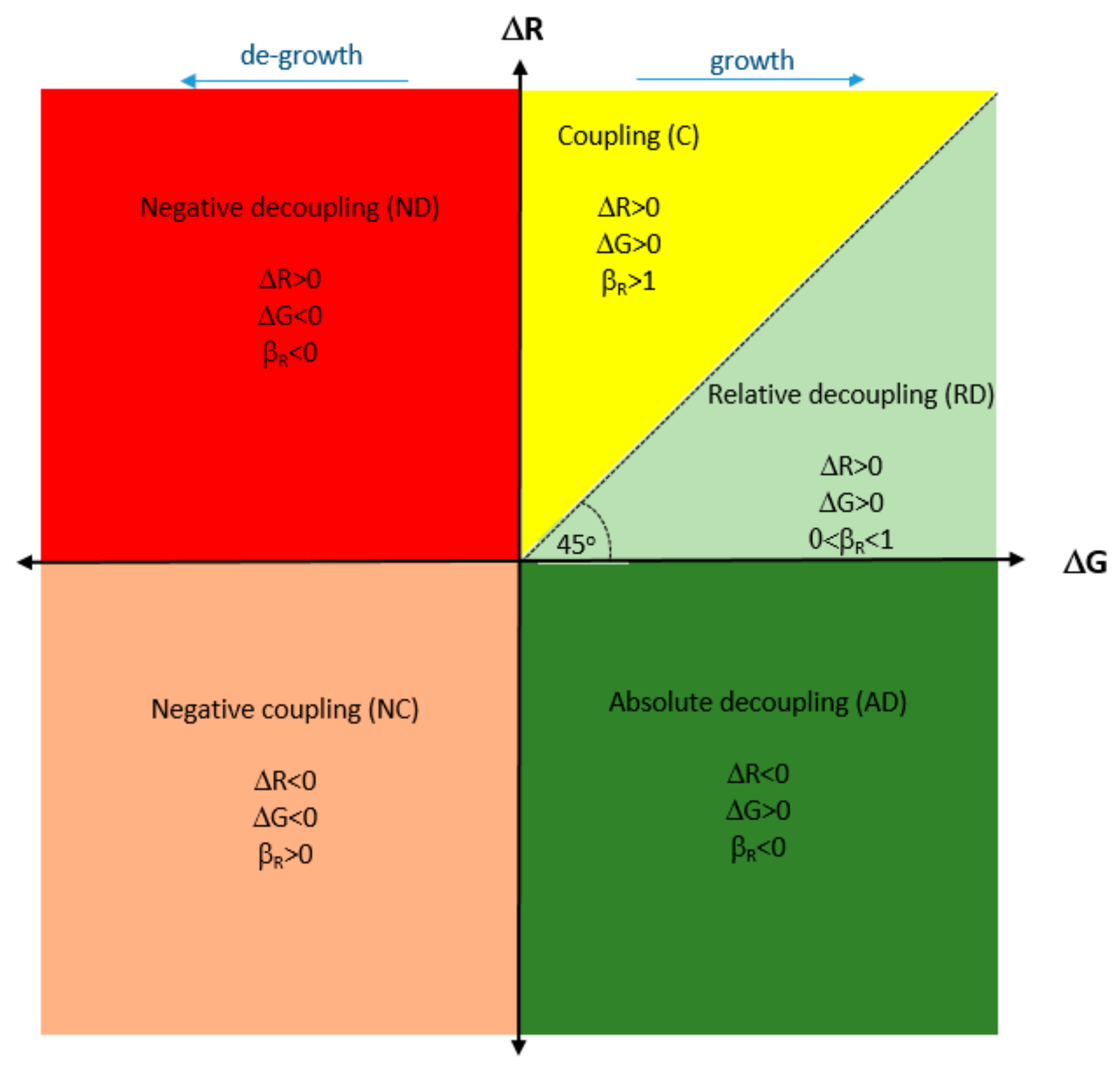
2.1. Tapio Decoupling Indicator
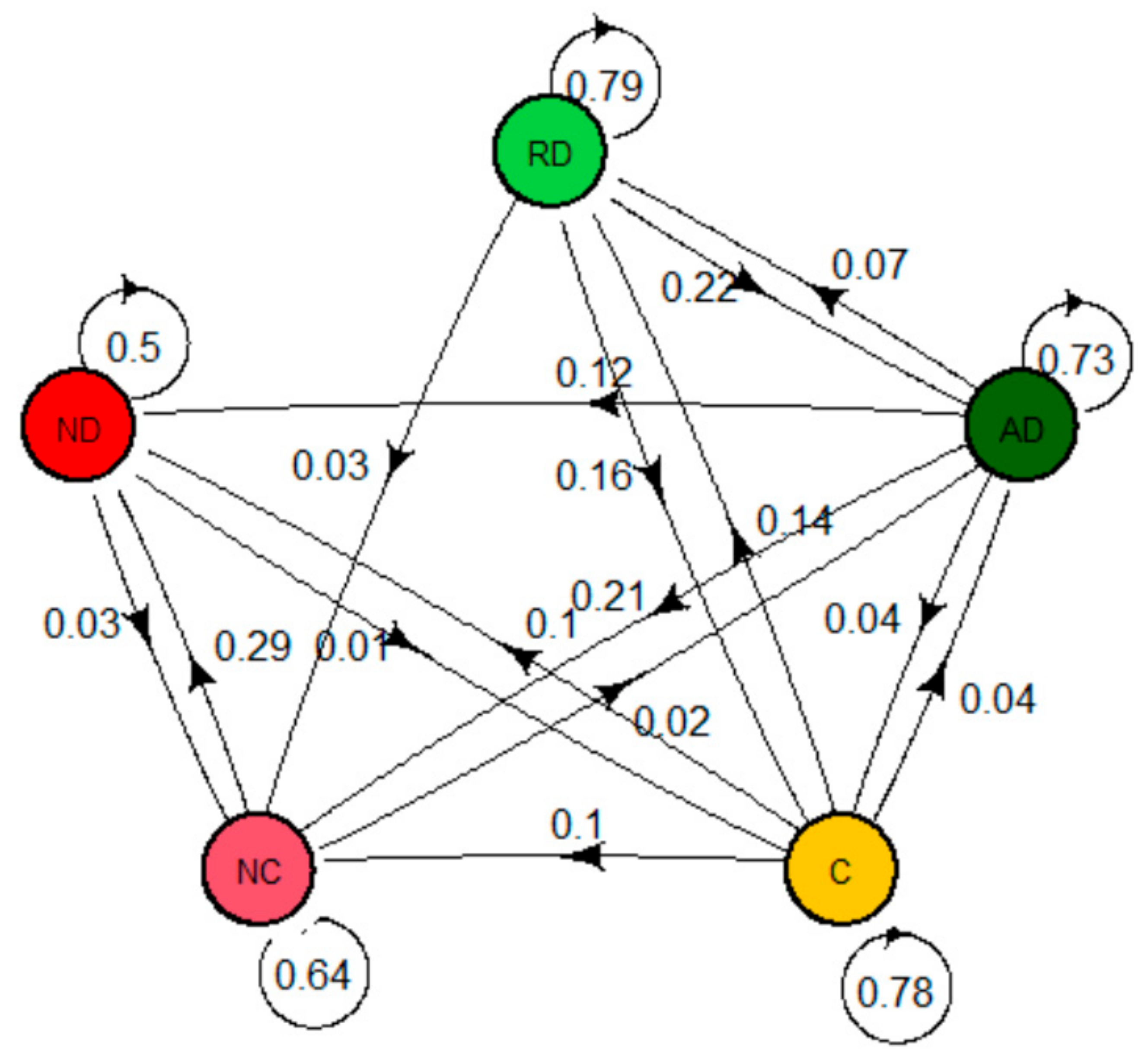
2.2. Markov Chain Model
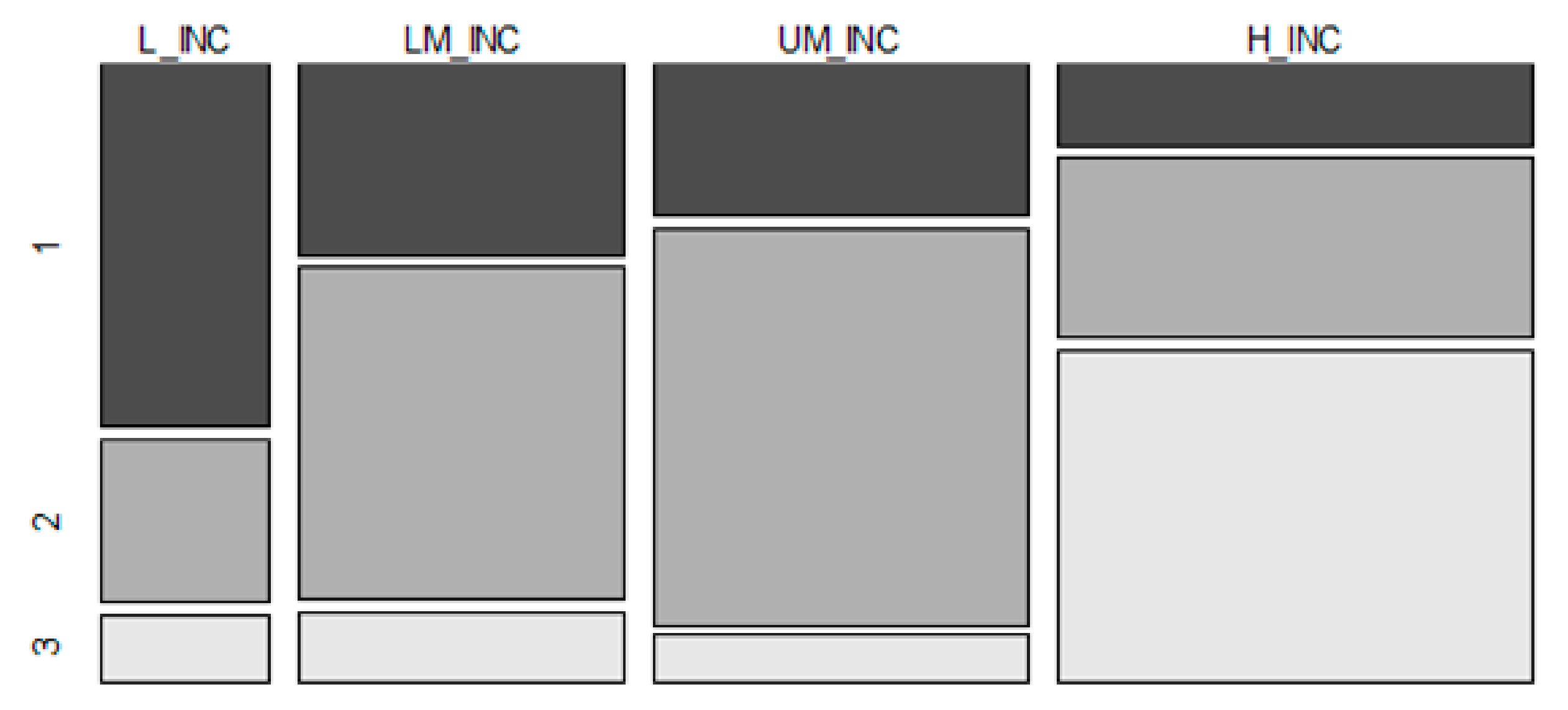
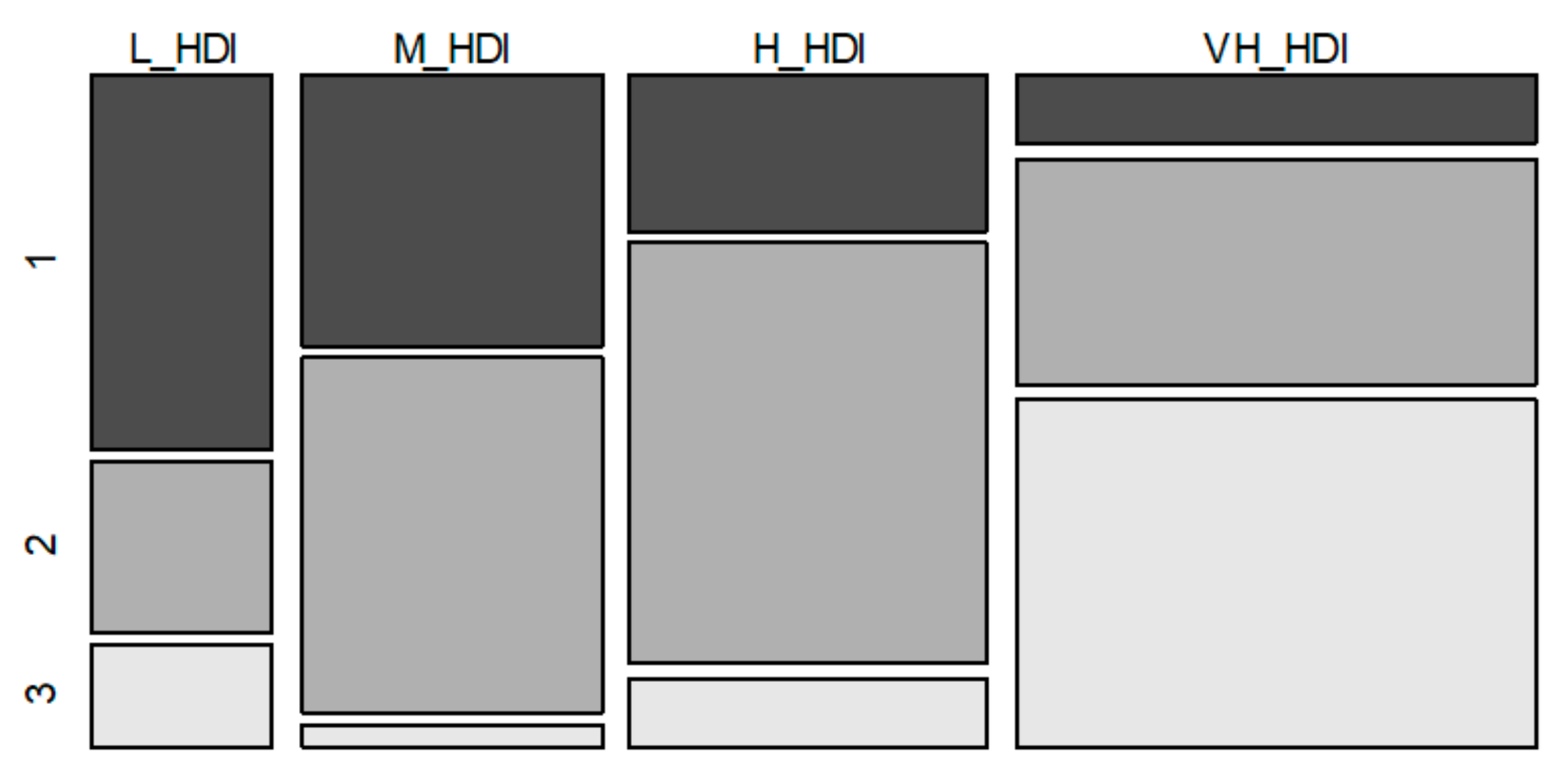
2.3. The PAM Clustering Method
2.4. Data
3. Results
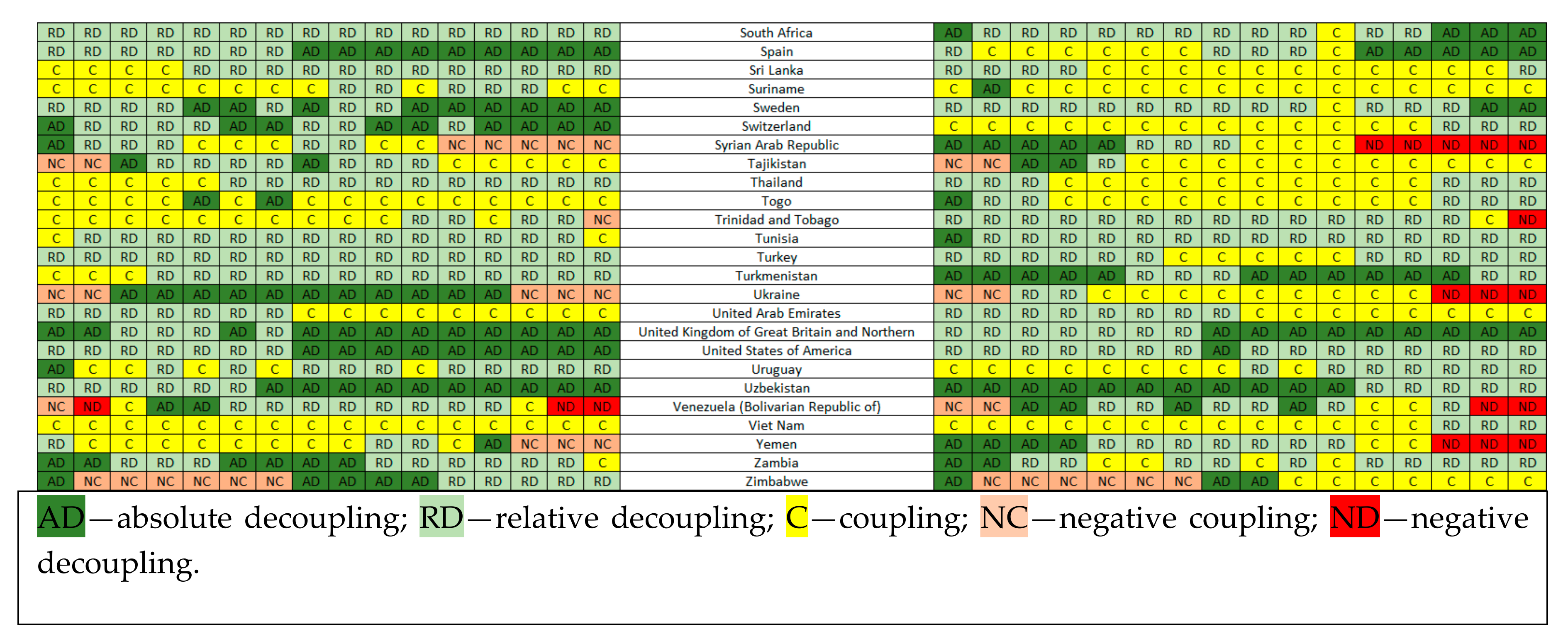
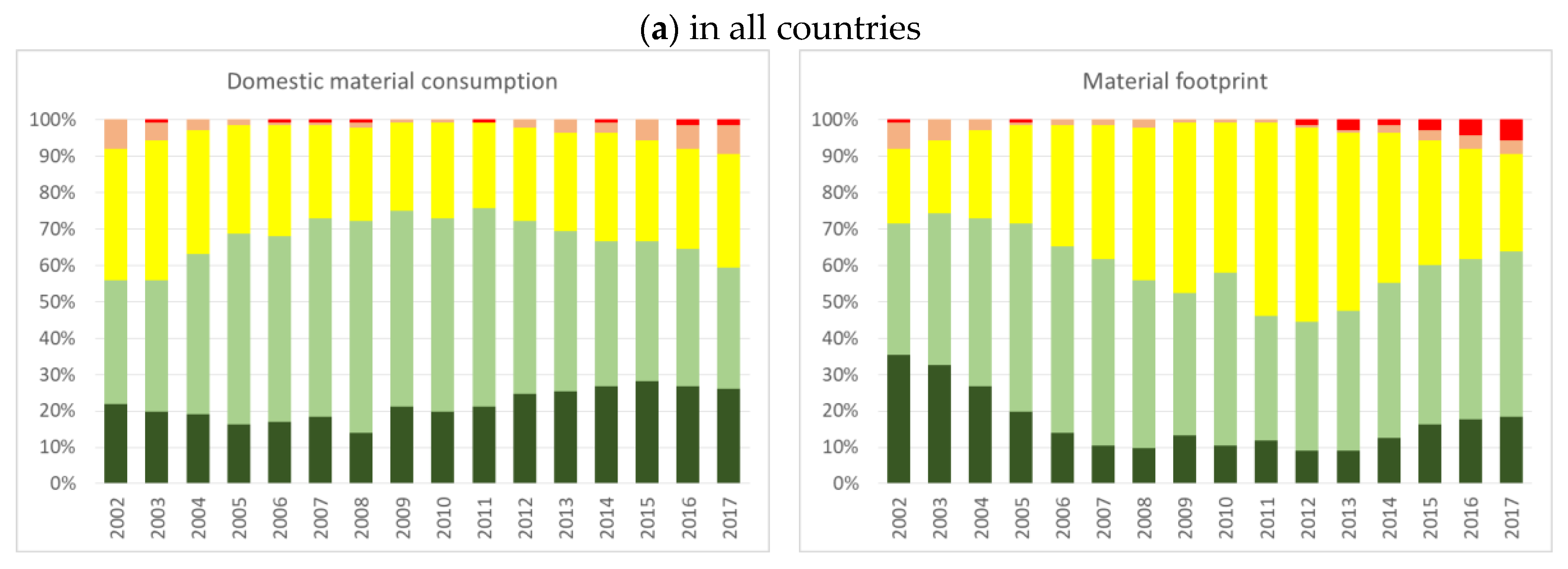
3.1. Tapio Results
3.2. Markov Chain Results
3.3. Clustering Results
4. Conclusions and Discussion
Author Contributions
Funding
Conflicts of Interest
Appendix A

| Year | 2002 | 2003 | 2004 | 2005 | 2006 | 2007 | 2008 | 2009 | 2010 | 2011 | 2012 | 2013 | 2014 | 2015 | 2016 | 2017 |
|---|---|---|---|---|---|---|---|---|---|---|---|---|---|---|---|---|
| in all countries | ||||||||||||||||
| AD | 22% | 20% | 19% | 16% | 17% | 18% | 14% | 21% | 20% | 21% | 25% | 26% | 27% | 28% | 27% | 26% |
| RD | 34% | 36% | 44% | 52% | 51% | 55% | 58% | 54% | 53% | 55% | 48% | 44% | 40% | 38% | 38% | 33% |
| C | 36% | 38% | 34% | 30% | 30% | 26% | 26% | 24% | 26% | 23% | 26% | 27% | 30% | 28% | 28% | 31% |
| NC | 8% | 5% | 3% | 1% | 1% | 1% | 1% | 1% | 1% | 0% | 2% | 4% | 3% | 6% | 6% | 8% |
| ND | 0% | 1% | 0% | 0% | 1% | 1% | 1% | 0% | 0% | 1% | 0% | 0% | 1% | 0% | 1% | 1% |
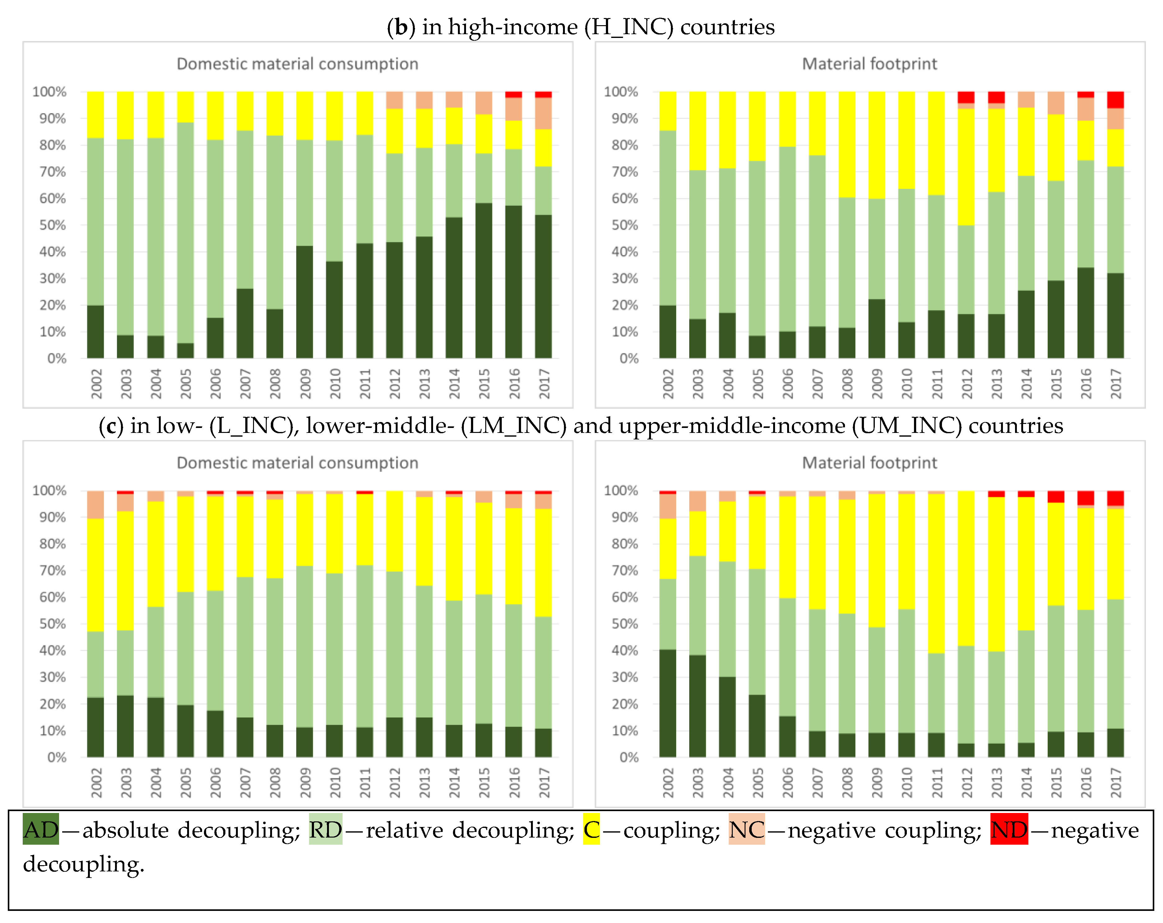
| in high-income (H_INC) countries | ||||||||||||||||
| AD | 20% | 9% | 9% | 6% | 15% | 26% | 19% | 42% | 36% | 43% | 44% | 46% | 53% | 58% | 57% | 54% |
| RD | 63% | 74% | 74% | 83% | 67% | 60% | 65% | 40% | 45% | 41% | 33% | 33% | 27% | 19% | 21% | 18% |
| C | 17% | 18% | 17% | 11% | 18% | 14% | 16% | 18% | 18% | 16% | 17% | 15% | 14% | 15% | 11% | 14% |
| NC | 0% | 0% | 0% | 0% | 0% | 0% | 0% | 0% | 0% | 0% | 6% | 6% | 6% | 8% | 9% | 12% |
| ND | 0% | 0% | 0% | 0% | 0% | 0% | 0% | 0% | 0% | 0% | 0% | 0% | 0% | 0% | 2% | 2% |
| in low- (L_INC), lower-middle- (LM_INC) and upper-middle-income (UM_INC) countries | ||||||||||||||||
| AD | 23% | 23% | 23% | 20% | 18% | 15% | 12% | 11% | 12% | 11% | 15% | 15% | 12% | 13% | 12% | 11% |
| RD | 25% | 24% | 34% | 42% | 45% | 53% | 55% | 60% | 57% | 61% | 55% | 49% | 47% | 48% | 46% | 42% |
| C | 42% | 45% | 40% | 36% | 35% | 30% | 30% | 27% | 30% | 27% | 30% | 33% | 39% | 34% | 36% | 41% |
| NC | 10% | 7% | 4% | 2% | 1% | 1% | 2% | 1% | 1% | 0% | 0% | 2% | 1% | 4% | 5% | 5% |
| ND | 0% | 1% | 0% | 0% | 1% | 1% | 1% | 0% | 0% | 1% | 0% | 0% | 1% | 0% | 1% | 1% |
| Year | 2002 | 2003 | 2004 | 2005 | 20a06 | 2007 | 2008 | 2009 | 2010 | 2011 | 2012 | 2013 | 2014 | 2015 | 2016 | 2017 |
|---|---|---|---|---|---|---|---|---|---|---|---|---|---|---|---|---|
| in all countries | ||||||||||||||||
| AD | 35% | 33% | 27% | 20% | 14% | 11% | 10% | 13% | 11% | 12% | 9% | 9% | 13% | 16% | 18% | 18% |
| RD | 36% | 42% | 46% | 52% | 51% | 51% | 46% | 39% | 48% | 34% | 35% | 38% | 43% | 44% | 44% | 45% |
| C | 21% | 20% | 24% | 27% | 33% | 37% | 42% | 47% | 41% | 53% | 53% | 49% | 41% | 34% | 30% | 27% |
| NC | 7% | 6% | 3% | 1% | 1% | 1% | 2% | 1% | 1% | 1% | 1% | 1% | 2% | 3% | 4% | 4% |
| ND | 1% | 0% | 0% | 1% | 0% | 0% | 0% | 0% | 0% | 0% | 1% | 3% | 1% | 3% | 4% | 6% |
| in high-income (H_INC) countries | ||||||||||||||||
| AD | 20% | 15% | 17% | 9% | 10% | 12% | 12% | 22% | 14% | 18% | 17% | 17% | 25% | 29% | 34% | 32% |
| RD | 66% | 56% | 54% | 66% | 69% | 64% | 49% | 38% | 50% | 43% | 33% | 46% | 43% | 38% | 40% | 40% |
| C | 14% | 29% | 29% | 26% | 21% | 24% | 40% | 40% | 36% | 39% | 44% | 31% | 25% | 25% | 15% | 14% |
| NC | 0% | 0% | 0% | 0% | 0% | 0% | 0% | 0% | 0% | 0% | 2% | 2% | 6% | 8% | 9% | 8% |
| ND | 0% | 0% | 0% | 0% | 0% | 0% | 0% | 0% | 0% | 0% | 4% | 4% | 0% | 0% | 2% | 6% |
| in low- (L_INC), lower-middle- (LM_INC) and upper-middle-income (UM_INC) countries | ||||||||||||||||
| AD | 41% | 38% | 30% | 24% | 16% | 10% | 9% | 9% | 9% | 9% | 5% | 5% | 6% | 10% | 10% | 11% |
| RD | 26% | 37% | 43% | 47% | 44% | 45% | 45% | 40% | 46% | 30% | 37% | 34% | 42% | 47% | 46% | 48% |
| C | 23% | 17% | 23% | 27% | 38% | 42% | 43% | 50% | 43% | 60% | 58% | 58% | 50% | 39% | 38% | 34% |
| NC | 9% | 7% | 4% | 1% | 2% | 2% | 3% | 1% | 1% | 1% | 0% | 0% | 0% | 0% | 1% | 1% |
| ND | 1% | 0% | 0% | 1% | 0% | 0% | 0% | 0% | 0% | 0% | 0% | 2% | 2% | 4% | 5% | 5% |
References
- Hickel, J.; Kallis, G. Is Green Growth Possible? New Political Econ. 2020, 25, 469–486. [Google Scholar] [CrossRef]
- OECD. Green Growth Indicators 2014; OECD: Paris, France, 2016. [Google Scholar] [CrossRef]
- Steininger, K.W.; Lininger, C.; Meyer, L.H.; Muñoz, P.; Schinko, T. Multiple carbon accounting to support just and effective climate policies. Nat. Clim. Chang. 2015, 6, 35–41. [Google Scholar] [CrossRef]
- Haberl, H.; Wiedenhofer, D.; Virág, D.; Kalt, G.; Plank, B.; Brockway, P.E.; Fishman, T.; Hausknost, D.; Krausmann, F.; Leon-Gruchalski, B.; et al. A systematic review of the evidence on decoupling of GDP, resource use and GHG emissions, part II: Synthesizing the insights. Environ. Res. Lett. 2020, 15, 065003. [Google Scholar] [CrossRef]
- Krausmann, F.; Gingrich, S.; Eisenmenger, N.; Erb, K.-H.; Haberl, H.; Fischer-Kowalski, M. Growth in global materials use, GDP and population during the 20th century. Ecol. Econ. 2009, 68, 2696–2705. [Google Scholar] [CrossRef]
- Fischer-Kowalski, M.; Krausmann, F.; Giljum, S.; Lutter, S.; Mayer, A.; Bringezu, S.; Moriguchi, Y.; Schütz, H.; Schandl, H.; Weisz, H. Methodology and indicators of economy-wide material flow accounting: State of the art and reliability across sources. J. Ind. Ecol. 2011, 15, 855–876. [Google Scholar] [CrossRef]
- Krausmann, F.; Schandl, H.; Eisenmenger, N.; Giljum, S.; Jackson, T. Material Flow Accounting: Measuring Global Material Use for Sustainable Development. Annu. Rev. Environ. Resour. 2017, 42, 647–675. [Google Scholar] [CrossRef]
- Wiedmann, T.; Schandl, H.; Lenzen, M.; Moran, D.; Suh, S.; West, J.; Kanemoto, K. The material footprint of nations. Proc. Natl. Acad. Sci. USA 2015, 112, 6271–6276. [Google Scholar] [CrossRef]
- Schaffartzik, A.; Eisenmenger, N.; Krausmann, F.; Weisz, H. Consumption-based material flow accounting: Austrian trade and consumption in raw material equivalents 1995–2007. J. Ind. Ecol. 2014, 18, 102–112. [Google Scholar] [CrossRef]
- Giljum, S.; Bruckner, M.; Martinez, A. Material Footprint Assessment in a Global Input-Output Framework. J. Ind. Ecol. 2014, 19, 792–804. [Google Scholar] [CrossRef]
- De Freitas, L.C.; Kaneko, S. Decomposing the decoupling of CO2 emissions and economic growth in Brazil. Ecol. Econ. 2011, 70, 1459–1469. [Google Scholar] [CrossRef]
- Wang, H.; Zhao, S.; Wei, Y.; Yue, Q.; Du, T. Measuring the Decoupling Progress in Developed and Developing Countries; Atlantis Press: Amsterdam, The Netherlands, 2018; pp. 377–381. [Google Scholar]
- Leal, P.A.; Marques, A.C.; Fuinhas, J.A. Decoupling economic growth from GHG emissions: Decomposition analysis by sectoral factors for Australia. Econ. Anal. Policy 2019, 62, 12–26. [Google Scholar] [CrossRef]
- Vadén, T.; Lähde, V.; Majava, A.; Järvensivu, P.; Toivanen, T.; Hakala, E.; Eronen, J. Decoupling for ecological sustainability: A categorisation and review of research literature. Environ. Sci. Policy 2020, 112, 236–244. [Google Scholar] [CrossRef]
- Wiedenhofer, D.; Virág, D.; Kalt, G.; Plank, B.; Streeck, J.; Pichler, M.; Mayer, A.; Krausmann, F.; Brockway, P.E.; Schaffartzik, A.; et al. A systematic review of the evidence on decoupling of GDP, resource use and GHG emissions, part I: Bibliometric and conceptual mapping. Environ. Res. Lett. 2020, 15, 063002. [Google Scholar] [CrossRef]
- Schandl, H.; Hatfield-Dodds, S.; Wiedmann, T.; Geschke, A.; Cai, Y.; West, J.; Newth, D.; Baynes, T.; Lenzen, M.; Owen, A. Decoupling global environmental pressure and economic growth: Scenarios for energy use, materials use and carbon emissions. J. Clean. Prod. 2016, 132, 45–56. [Google Scholar] [CrossRef]
- Shao, Q.; Schaffartzik, A.; Mayer, A.; Krausmann, F. The high ‘price’ of dematerialization: A dynamic panel data analysis of material use and economic recession. J. Clean. Prod. 2017, 167, 120–132. [Google Scholar] [CrossRef]
- Bithas, K.; Kalimeris, P. Unmasking decoupling: Redefining the Resource Intensity of the Economy. Sci. Total. Environ. 2018, 620, 338–351. [Google Scholar] [CrossRef]
- Wu, Z.; Schaffartzik, A.; Shao, Q.; Wang, D.; Li, G.; Su, Y.; Rao, L. Does economic recession reduce material use? Empirical evidence based on 157 economies worldwide. J. Clean. Prod. 2019, 214, 823–836. [Google Scholar] [CrossRef]
- Agnolucci, P.; Flachenecker, F.; Söderberg, M. The causal impact of economic growth on material use in Europe. J. Environ. Econ. Policy 2017, 6, 415–432. [Google Scholar] [CrossRef]
- Telega, I.; Telega, A. Driving factors of material consumption in European countries—Spatial panel data analysis. J. Environ. Econ. Policy 2019, 9, 1–12. [Google Scholar] [CrossRef]
- Steinberger, J.K.; Krausmann, F.; Getzner, M.; Schandl, H.; West, J. Development and Dematerialization: An International Study. PLoS ONE 2013, 8, e70385. [Google Scholar] [CrossRef]
- Wang, H.; Hashimoto, S.; Yue, Q.; Moriguchi, Y.; Lu, Z. Decoupling analysis of four selected countries: China, Russia, Japan, and the United States during 2000–2007. J. Ind. Ecol. 2013, 17, 618–629. [Google Scholar] [CrossRef]
- Liu, G.; Jia, F.; Yue, Q.; Ma, D.; Pan, H.; Wu, M. Decoupling of nonferrous metal consumption from economic growth in China. Environ. Dev. Sustain. 2015, 18, 221–235. [Google Scholar] [CrossRef]
- Wang, Z.; Feng, C.; Chen, J.; Huang, J.-B. The driving forces of material use in China: An index decomposition analysis. Resour. Policy 2017, 52, 336–348. [Google Scholar] [CrossRef]
- Martinico-Perez, M.F.G.; Schandl, H.; Fishman, T.; Tanikawa, H. The Socio-Economic Metabolism of an Emerging Economy: Monitoring Progress of Decoupling of Economic Growth and Environmental Pressures in the Philippines. Ecol. Econ. 2018, 147, 155–166. [Google Scholar] [CrossRef]
- Wu, Y.; Zhu, Q.; Zhu, B. Comparisons of decoupling trends of global economic growth and energy consumption between developed and developing countries. Energy Policy 2018, 116, 30–38. [Google Scholar] [CrossRef]
- Salahuddin, M.; Gow, J. Economic growth, energy consumption and CO2 emissions in Gulf Cooperation Council countries. Energy 2014, 73, 44–58. [Google Scholar] [CrossRef]
- Stevens, P.; Lahn, G.; Kooroshy, J. The Resource Curse Revisited; Chatham House: London, UK, 2015. [Google Scholar]
- Schaffartzik, A.; Wiedenhofer, D.; Eisenmenger, N. Raw Material Equivalents: The Challenges of Accounting for Sustainability in a Globalized World. Sustainability 2015, 7, 5345–5370. [Google Scholar] [CrossRef]
- Schandl, H.; Fischer-Kowalski, M.; West, J.; Giljum, S.; Dittrich, M.; Eisenmenger, N.; Geschke, A.; Lieber, M.; Wieland, H.; Schaffartzik, A.; et al. Global Material Flows and Resource Productivity: Forty Years of Evidence. J. Ind. Ecol. 2017, 22, 827–838. [Google Scholar] [CrossRef]
- Ward, J.; Sutton, P.C.; Werner, A.D.; Costanza, R.; Mohr, S.H.; Simmons, C.T. Is Decoupling GDP Growth from Environmental Impact Possible? PLoS ONE 2016, 11, e0164733. [Google Scholar] [CrossRef]
- Fletcher, R.; Rammelt, C. Decoupling: A Key Fantasy of the Post-2015 Sustainable Development Agenda. Globalizations 2016, 14, 450–467. [Google Scholar] [CrossRef]
- Kan, S.; Chen, B.; Chen, B. Worldwide energy use across global supply chains: Decoupled from economic growth? Appl. Energy 2019, 250, 1235–1245. [Google Scholar] [CrossRef]
- Tapio, P. Towards a theory of decoupling: Degrees of decoupling in the EU and the case of road traffic in Finland between 1970 and 2001. Transp. Policy 2005, 12, 137–151. [Google Scholar] [CrossRef]
- Kaufman, L.; Rousseeuw, P.J. Partitioning Around Medoids (Program PAM); Wiley: Hoboken, NJ, USA, 2008; pp. 68–125. [Google Scholar]
- Malik, A.; Lan, J. The role of outsourcing in driving global carbon emissions. Econ. Syst. Res. 2016, 28, 168–182. [Google Scholar] [CrossRef]
- OECD. Indicators to Measure Decoupling of Environmental Pressure from Economic Growth; Sustainable Development SG/SD(2002)1; OECD: Paris, France, 2002. [Google Scholar]
- UNEP. Decoupling Natural Resource Use and Environmental Impacts from Economic Growth; A Report of the Working Group on Decoupling to the International Resource, Panel; Fischer-Kowalski, M., Swilling, M., von Weizsäcker, E.U., Ren, Y., Moriguchi, Y., Crane, W., Krausmann, F., Eisenmenger, N., Giljum, S., Hennicke, P., et al., Eds.; UNEP—Sustainable Consumption and Production Branch: Paris, France, 2011. [Google Scholar]
- Lu, Z.; Wang, H.; Yue, Q. Decoupling Indicators: Quantitative Relationships between Resource Use, Waste Emission and Economic Growth. Resour. Sci. 2011, 33, 2–9. (In Chinese) [Google Scholar]
- Naqvi, A.A.; Zwickl, K. Fifty shades of green: Revisiting decoupling by economic sectors and air pollutants. Ecol. Econ. 2017, 133, 111–126. [Google Scholar] [CrossRef]
- Everitt, B.; Landau, S.; Leese, M.; Stahl, D. Cluster Analysis, 5th ed.; Wiley: Hoboken, NJ, USA, 2011. [Google Scholar]
- Rousseeuw, P.J. Silhouettes: A graphical aid to the interpretation and validation of cluster analysis. J. Comput. Appl. Math. 1987, 20, 53–65. [Google Scholar] [CrossRef]
- Lenzen, M.; Moran, D.; Kanemoto, K.; Geschke, A. Building Eora: A Global Multi-Region Input–Output Database at High Country And Sector Resolution. Econ. Syst. Res. 2013, 25, 20–49. [Google Scholar] [CrossRef]
- Kalimeris, P.; Bithas, K.; Richardson, C.; Nijkamp, P. Hidden linkages between resources and economy: A “Beyond-GDP” approach using alternative welfare indicators. Ecol. Econ. 2020, 169, 106508. [Google Scholar] [CrossRef]
- World Bank. 2019. World Development Indicators database. Washington, DC. Available online: http://data.worldbank.org (accessed on 15 September 2020).
- Human Development Reports. Available online: http://hdr.undp.org/en/indicators/137506 (accessed on 15 September 2020).
- Human Development Reports—Technical Notes. Available online: http://hdr.undp.org/sites/default/files/hdr2019_technical_notes.pdf (accessed on 15 September 2020).


| State | ||||
|---|---|---|---|---|
| Negative decoupling | Expansive negative decoupling | + | + | (1.2, + ∞) |
| Strong negative decoupling | + | − | (−∞, 0) | |
| Weak negative decoupling | − | − | [0, 0.8) | |
| Decoupling | Weak decoupling | + | + | [0, 0.8) |
| Strong decoupling | − | + | (−∞, 0) | |
| Recessive decoupling | − | − | (1.2, + ∞) | |
| Coupling | Expansive coupling | + | + | [0.8, 1.2] |
| Recessive coupling | − | − | [0.8, 1.2] |
| Group | No of Countries | Medoid | Decoupling Trend |
|---|---|---|---|
| 1 | 39 | Vietnam |  |
| 2 | 63 | Turkey |  |
| 3 | 39 | United States of America |  |
| Group | No of Countries | Medoid | Decoupling Trend |
|---|---|---|---|
| 1 | 44 | Lithuania |  |
| 2 | 28 | Peru |  |
| 3 | 14 | Oman |  |
| 4 | 55 | India |  |
Publisher’s Note: MDPI stays neutral with regard to jurisdictional claims in published maps and institutional affiliations. |
© 2020 by the authors. Licensee MDPI, Basel, Switzerland. This article is an open access article distributed under the terms and conditions of the Creative Commons Attribution (CC BY) license (http://creativecommons.org/licenses/by/4.0/).
Share and Cite
Frodyma, K.; Papież, M.; Śmiech, S. Decoupling Economic Growth from Fossil Fuel Use—Evidence from 141 Countries in the 25-Year Perspective. Energies 2020, 13, 6671. https://doi.org/10.3390/en13246671
Frodyma K, Papież M, Śmiech S. Decoupling Economic Growth from Fossil Fuel Use—Evidence from 141 Countries in the 25-Year Perspective. Energies. 2020; 13(24):6671. https://doi.org/10.3390/en13246671
Chicago/Turabian StyleFrodyma, Katarzyna, Monika Papież, and Sławomir Śmiech. 2020. "Decoupling Economic Growth from Fossil Fuel Use—Evidence from 141 Countries in the 25-Year Perspective" Energies 13, no. 24: 6671. https://doi.org/10.3390/en13246671
APA StyleFrodyma, K., Papież, M., & Śmiech, S. (2020). Decoupling Economic Growth from Fossil Fuel Use—Evidence from 141 Countries in the 25-Year Perspective. Energies, 13(24), 6671. https://doi.org/10.3390/en13246671