An Interval Mathematic-Based Methodology for Reliable Resilience Analysis of Power Systems in the Presence of Data Uncertainties

Abstract

Prevention and mitigation of low probability, high impact events is becoming a priority for power system operators, as natural disasters are hitting critical infrastructures with increased frequency all over the world. Protecting power networks against these events means improving their resilience in planning, operation and restoration phases. This paper introduces a framework based on time-varying interval Markov Chains to assess system’s resilience to catastrophic events. After recognizing the difficulties in accurately defining transition probabilities, due to the presence of data uncertainty, this paper proposes a novel approach based on interval mathematics, which allows representing the elements of the transition matrices by intervals, and computing reliable enclosures of the transient state probabilities. The proposed framework is validated on a case study, which is based on the resilience analysis of a power system in the presence of multiple contemporary faults. The results show how the proposed framework can successfully enclose all the possible outcomes obtained through Monte Carlo simulation. The main advantages are the low computational burden and high scalability achieved.

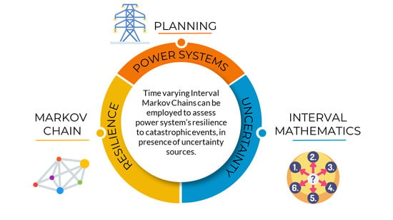
1. Introduction

Power systems were traditionally planned and operated according to security and reliability principles, which involved the analysis of credible events, such as N-1 or N-2 contingencies.

However, due to the increasing frequency of natural disasters [1,2] and the greater vulnerability of power systems to cyber-attacks [3], planning studies and operational paradigms are changing. Hence, researchers and power system operators are increasingly interested to the concept of resilience [4].

Resilience is defined by the IEEE as [5]: the ability to withstand and reduce the magnitude and/or duration of disruptive events, which include the capability to anticipate, absorb, adapt to, and/or rapidly recover from such an event.

On the basis of this definition, resilience studies can be classified in three main branches [6]:

• The ability to anticipate High Impact Low Probability (HILP) events is addressed in resilience-based planning, which aims at identifying long-term strategies to strengthen power networks.
• The capacity to absorb and adapt is analysed in resilience-based response, which aims at improving power system operation in terms of reserves, network topology control, vulnerability analyses.
• Finally, the ability to recover from a catastrophic event, is explored in resilience-based restoration analysis, which aims at minimizing the impacts of power outage after a catastrophic event.

Although the scientific literature proposes a wide range of quantitative and qualitative methods and metrics to assess resilience, it is still lacking a global consensus over a unified framework [7]. Qualitative evaluation is based on questionnaires, investigations, ratings from Transmission System Operators, and overall considerations regarding correlated systems, such as fuel supply chain or telecommunication systems. The results are analyzed through qualitative planning methods, such as Analytic Hierarchy Process (AHP), in decision making tools [8].

On the other hand, quantitative methods introduce metrics to compare the level of resilience of different systems. They can be simulation-based, analytical or based on statistical analysis of historical data.

The main metrics aim at evaluating the difference between the expected system performance and the real system performance under a HILP event. Some examples are restoration costs, restoration time or loss of load frequency and loss of load expectation [9].

In particular, the authors of Reference [10], show how the definition of resilience implies a dependency on time—a broad classification can be done between short-term and long-term resilience. Short-term resilience refers to the characteristics that the power system should have before, during and after a HILP contingency, while long-term resilience refers to the adaptability of the system to unknown future threats. The latter can be achieved by performing multiple risk and reliability studies, and planning ahead for unexpected events.

Resilience is a concept that is strictly related to mitigation, which is the process of reducing the unavoidable damage suffered by a system due to a HILP event. Mitigation strategies vary depending on the considered time-scale. They can be evaluated during the planning and operation phase, and they are mainly classified in physical interventions on the network to improve its overall robustness, or implementation of more advanced monitoring and control capabilities [11]. Examples of actions aimed at reducing the impact of unexpected events in the long run are [12]:

• Operational procedures: risk assessment and evaluation of mitigation strategies.
• Weather estimation: considering location and severity.
• Components’ upgrade: by replacing old ones or adding redundancy where needed.
• Relocation: by rerouting lines or moving critical components to areas less affected by HILP events.
• Increased awareness: by introducing advanced monitoring tools.

In all these contexts, the analysis of the potential impacts of renewable energy sources (RES) is an interesting open problem to address. In particular, although the use of different, decentralized RES can be beneficial for the power system in mitigating the impacts of HILP events, their intermittent power profiles, the limited black start capability, and the misoperation of traditional coordinated protections, are some of the most critical issues hindering the RES contributions to resiliency enhancement, especially in long-term planning scenarios. In this domain, the research for reliable computing paradigms aimed at managing the uncertainties induced by both RES and other relevant sources, for example, weather dependent fault/reparation rates, represents a relevant issue to address.

A model often used to deal with resilience-based planning problems is based on Markov processes [13,14], which are employed in the task of modelling the system states evolution consequent to HILP events, once the deterministic transition probabilities are assessed. Anyway, the reliable estimation of these parameters is a challenging issue to address, especially in predictive resilience studies, which are mainly related to low frequency events. In this context, the available historical information are often not enough to reliably describe the state transition rates by deterministic variables. To face this issue, sampling-based approaches, such as Monte Carlo simulations, could be a useful solution strategy, but the associated computational burden, especially for large-scale systems, makes them unfeasible for practical purposes. Furthermore, stochastic models often need assumptions about the probability distributions of the uncertain variables, which are typically assumed Gaussian, although this assumption is often not supported by experimental evidence [15].

To overcome these limitations, stochastic models could be enhanced by advanced modelling approaches, such as convex models [16]. A convex model is a set-theoretic approach, which aims at modelling the data uncertainty by defining subsets over the set of allowed events. No probability measure is defined over the set, such as in the case of probabilistic approaches. An instance of convex models for handling uncertainty is interval mathematics [17], which considers hypercubes as convex sets to describe uncertainty.

Interval Mathematics (IM) was first introduced to handle the uncertainty raising from numeric computations [18], however it spread over different disciplines as an alternative tool to deal with stochastic behaviours or inaccurate models. It was deployed in different power systems and power electronics applications, such as load flow [19] or power converter’s characteristics [20]. IM was also applied to model uncertain Markov Chains, typically referred as Interval Markov Chains, where the state transition probabilities are uncertain but bounded in fixed real-value intervals [21]. This methodology could play an important role in resilience-based long term planning and mitigation, where the long time-horizon, the scarcity of data characterizing HILP events, and the large number of analyzed scenarios, require the conceptualization of reliable computing techniques, which allow overcoming the intrinsic limitations of homogeneous, deterministic Markov Chains.

Armed with such a vision, in this paper Interval Markov Chains will be adopted for modelling uncertain time-varying models applied to resilience-based long term planning and mitigation. The main advantage deriving by the application of this computing paradigm is its low computational burden, which grants large scalability levels, and its robustness, since it allows to reliably compute an outer estimation of all possible outcomes of a given set of random scenarios, considering all the possible combinations of the uncertain variables.

The paper is organized as follows: Section 2 describes the mathematical methods employed for the analysis, such as Markov Chains, Interval Mathematics and finally Interval Markov Chains, Section 3 presents the case study aimed at validating the proposed methodology, Section 4 suggests future directions for research on this topic and Section 5 draws the main conclusions from the results.

2. Methods

2.1. Markov Chains

A Markov Chain is a stochastic dynamic process $X\left(t\right):x\ge 0$ which satisfies the Markov property:

$$P(X_t=x_t|X_{t-1}=x_{t-1},\dots ,X_0=x_0)=P(X_t=x_t|X_{t-1}=x_{t-1}).$$

(1)

Hence $X\left(t\right)$, which is a variable representing the state s occupied over the time t in a random occurrence, evolves based only on its present state.

Markov Chains can model both discrete and continuous processes and the number of states can be infinite or finite.

Discrete-Time Markov Chains

In this paper, the analysis will be focused on discrete time Markov Chains. A Discrete Time Markov Chain describes the evolution of a system over a set $\mathcal{S}$ of N states, $\mathcal{S}=\{s_1,\dots ,s_N\}$. At each time t, the system can be only in a single state. The probability that the system is in the state $s_i$ at time t is given by the state probability ${\pi }_i\left(t\right)$. Since each state is characterized by a state probability and these probabilities vary over time, a vector $\Pi \left(t\right)=\{{\pi }_1\left(t\right),\dots ,{\pi }_N\left(t\right)\}$ of state probabilities is defined for each step t of the evolution over time [22].

State probabilities are strictly related to transition probabilities $p_{ij}\left(t\right)$, which describe the probability that the system evolves from state $s_i$ to state $s_j$ at time t.

Transition probabilities can be constant or vary over time. In the first case the Markov Chain is called homogeneous. In this paper, we will deal with time-varying transition probabilities [23].

The transition matrix $\mathit{P}\left(t\right)$ is a square matrix of dimension n, where n is the number of possible states. It contains the set of transition probabilities from a state to another. The transition matrix is stochastic, since each of its elements belongs to the interval $[0,1]$, and each row of the matrix $\mathit{P}\left(t\right)$ satisfies the condition:

$$\sum _{j=1}^n{p}_{ij}=1.$$

(2)

The trajectory of the state probabilities from an initial step to a certain time T, can be obtained by solving a finite difference equation for each time step t:

$$\pi (t+1)=\mathit{P}\left(t\right)·\pi \left(t\right).$$

(3)

Markov Chains find different applications in power system engineering, such as the analysis of voltage profiles [24], characterization of the harmonics [25] or analysis of the electrical vehicles [26] to name some.

2.2. Effects of Data Uncertainties

Transition matrices, which rule the evolution of Markov Chains, are commonly described by deterministic real-valued coefficients. Such a description does not consider the large amount of uncertainty sources which affect transition rates. For example, the potential sources of uncertainty within power systems include natural temporal variations, monitoring and forecasting errors, wrong estimation of physical parameters [15]. Uncertainty can be either aleatory or epistemic: aleatory uncertainty is irreducible, since it is inherited from the random behaviour of the considered process. Epistemic uncertainty can be reduced by improving the accuracy of the models or the estimation of the parameters.

An example of epistemic uncertainty is the estimation of transition rates that results from a limited amount of available data. For example some influencing variables might be known with low accuracy or they might not even be measurable [27]. Another source of epistemic uncertainty is due to the classification of continuous variables into discrete classes: the distinction between the classes might not always be trivial, especially for boundary values.

Uncertainty can be represented with different methods. The most common is the probabilistic model, however it might not always be correctly quantifiable. Furthermore, exogenous variables, which influence transition rates, might not be easily represented in probabilistic form.

A wiser approach, in case there is no accurate probabilistic representation of a process, is to represent the transition matrix as an interval matrix: that is, a matrix whose elements are interval variables [28]. The following section presents the mathematical framework under which interval Markov Chains can be defined.

2.3. Interval Mathematics

Interval mathematics has been widely used in the scientific literature to address uncertain computations in different engineering branches [29,30,31]. With respect to power system engineering, some examples of its application have been described by References [32,33,34].

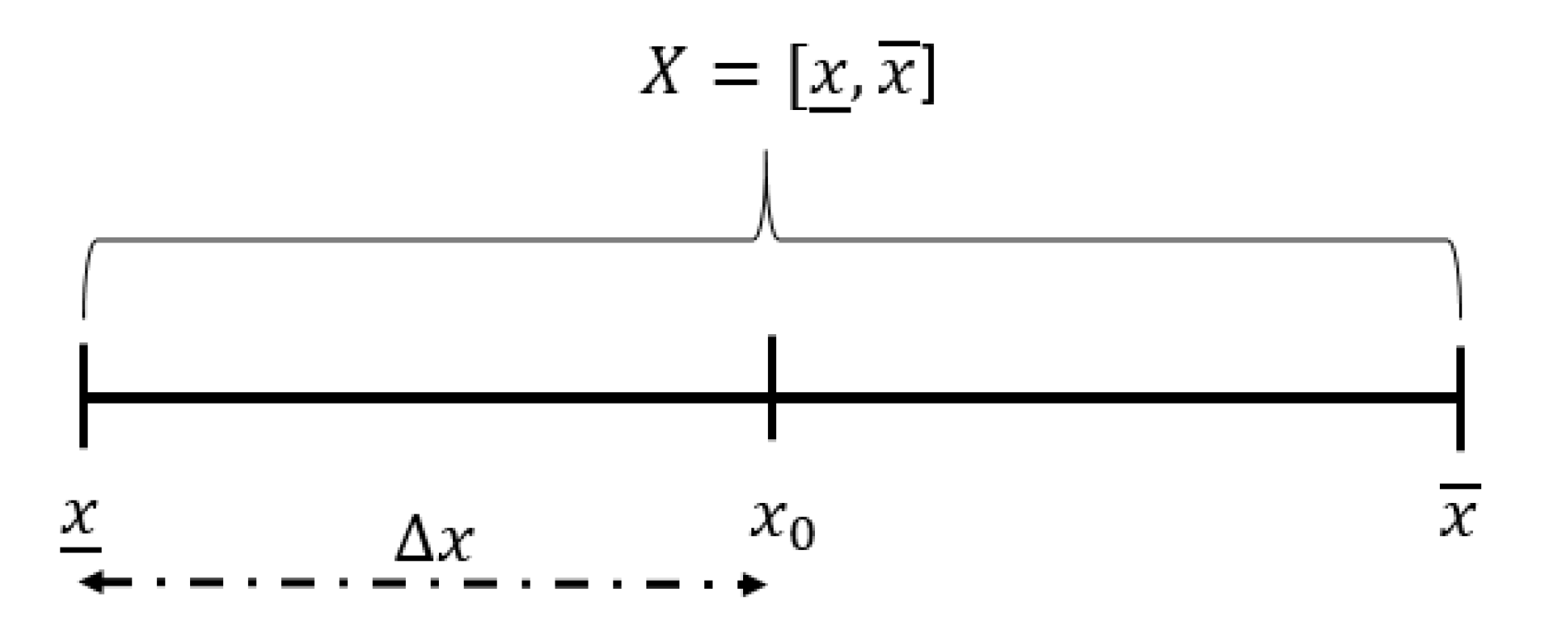
Given the field of real numbers $\mathbb{R}$, an interval is a subset of $\mathbb{R}$ of the form [35]:

$$A=[\underline{a},\overline{a}]=\{x:\underline{a}\le x\le \overline{a},\underline{a},\overline{a}\in \mathbb{R}\}.$$

(4)

The numbers $\underline{a}$ and $\overline{a}$ represent the lower and upper values of the interval. The set of all closed intervals in $\mathbb{R}$ can be called $\mathcal{I}\left(\mathbb{R}\right)$. A graphical representation is shown in Figure 1. Real numbers can be considered a particular instance of $\mathcal{I}\left(\mathbb{R}\right)$, in which $\underline{a}=\overline{a}$.

Binary operations can be defined for $\mathcal{I}\left(\mathbb{R}\right)$. Given two intervals: A and B, basic operations are:

$$\begin{array}{cc}\hfill & A+B=[\underline{a}+\underline{b},\overline{a}+\overline{b}]\hfill \\ \hfill & A-B=[\underline{a}-\overline{b},\overline{a}-\underline{b}]\hfill \\ \hfill & A·B=[min(\underline{a}\underline{b},\underline{a}\overline{b},\overline{a}\underline{b},\overline{a}\overline{b}),max(\underline{a}\underline{b},\underline{a}\overline{b},\overline{a}\underline{b},\overline{a}\overline{b})]\hfill \\ \hfill & A:B=[\underline{a},\overline{a}]·[\frac{1}{\overline{b}},\frac{1}{\underline{b}}]\hfill \\ \hfill & kA=[k\underline{a},k\overline{a}].\hfill \end{array}$$

(5)

The interval can also be characterized by a central value $x_0$, a width $w\left(X\right)$ and a radius $\Delta x$:

$$x_0=\frac{1}{2}[\underline{x}+\overline{x}]$$

(6)

$$w\left(X\right)=\overline{x}-\underline{x}$$

(7)

$$\Delta x=\frac{1}{2}[\overline{x}-\underline{x}].$$

(8)

In the analysis of uncertain problems, the central value is usually taken as the value considered in case of a deterministic model. The radius depends on the degree of uncertainty of the parameter considered: greater uncertainty involves a larger radius.

An issue to deal with in interval analysis is the dependency problem [36]. When an interval variable appears more than once in computations, it is treated as a different and independent variable at each step of the computation [37]. Namely, in case of the product $X·X$, given x as an unknown number known to lie within the interval X, the product $x·x$ does not imply that the first factor is the same as the second: they vary independently and this causes the widening of the resulting interval. For example, given the interval $X=[-1,1]$, the correct value for $X^2$ would be $X^2=[0,1]$. However, due to the dependency problem, by applying Equation (5), $X^2=[-1,1]$, which contains the correct interval solution, but is wider.

A simple means to reduce the dependency problem is to rewrite, when possible, the expression to be computed in a way that equal variables appear only once. If overconservatism must be avoided, it is possible to apply affine arithmetic [38], at the cost of increased computational burden. Affine arithmetic maintains the dependencies between variables even after computations which would normally lead to wider intervals.

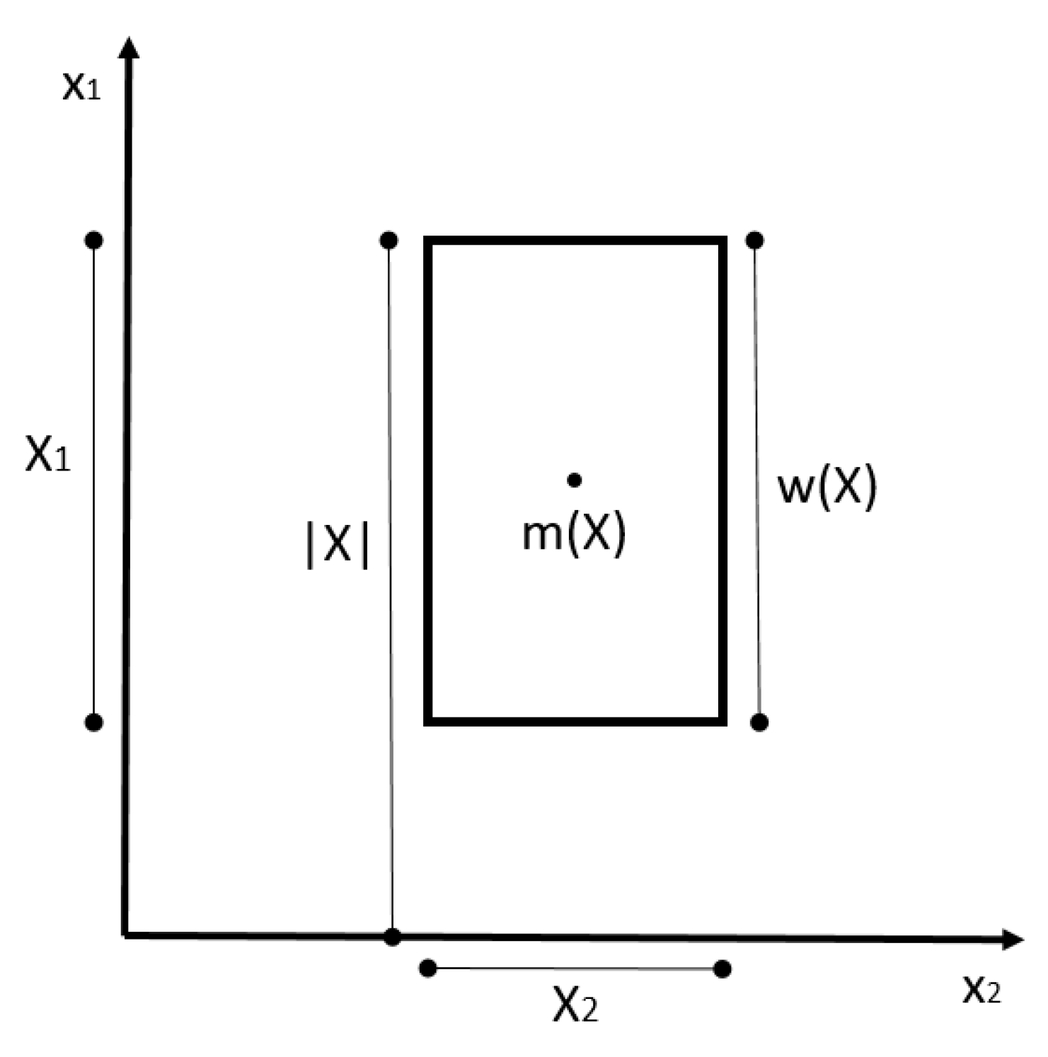
Interval mathematics can be extended to more than one dimension. An interval vector is a vector whose components are interval elements. For example, in case of a two dimensional interval vector X:

$$X=\{X_1,X_2\}=\{[{\underline{x}}_1,{\overline{x}}_1],[{\underline{x}}_2,{\overline{x}}_2]\}.$$

(9)

The geometrical representation of that vector is a rectangle in the plane, as shown in Figure 2 that is, it is the set of all the points $(x_1,x_2)$ such that:

$${\underline{X}}_1\le x_1\le {\overline{X}}_1{\underline{X}}_2\le x_2\le {\overline{X}}_2.$$

(10)

For an interval vector, the following quantities can be defined:

• The width of the interval vector $w\left(X\right)$, that is the largest of the widths of its component intervals:

  $$w\left(X\right)=\underset{i}{max}w\left(X_i\right)$$

  (11)
• The norm, which is a generalization of the absolute value:

  $$\left|X\right|=\underset{i}{max}\left|X_i\right|$$

  (12)
• The midpoint, which is the point corresponding to the central values:

  $$m\left(X\right)=(x_{0,1},x_{0,2},\dots ,x_{0,n}).$$

  (13)

Similarly, a matrix whose elements are intervals is called interval matrix. An interval matrix can be considered as a set of point matrices.

2.4. Interval Markov Chains

Transition probabilities and initial state probabilities of a Markov Chain might not be known with the desired degree of accuracy. The traditional approach to handle the uncertainty is to take the best estimates of the parameters, however the reliability of this approach is questionable. When considering high risk situations, such as in resilience studies including HILP events, such unreliability should be minimized, in order to avoid huge losses.

A solution to overcome the unreliability problem is the incorporation of imprecision into the model. This can be achieved in two ways [39]:

• The assumption of time homogeneity, that is, transition probabilities considered constant over time, can be preserved, but they are considered imprecisely known [40,41].
• Classical models can be further improved by omitting the assumption of time homogeneity, as in the case of Markov set-chains theory [42].

In general, the described approaches involve the substitution of single and precisely known transition probabilities with sets of feasible probabilities. Modelling capabilities depend on the form used to represent such sets, which is connected to the constraints used to determine them.

The most common form of sets are intervals of probabilities: the transition probability $p_{ij}$ from state i to j is given in the form of interval $[{\underline{p}}_{ij},{\overline{p}}_{ij}]$, which is supposed to contain the unknown true transition probability. Although true transition probabilities are unknown, the values within intervals must be taken such that they sum to 1. Furthermore, a fundamental assumption to work with intervals is that all values of the interval must be reachable, that is, the property of coherence is satisfied.

Interval Markov chains map elementary events, which are the target states, to intervals of probabilities [40]. The theory of interval probabilities was developed by Weichselberger [43], and the main elements of this theory are illustrated below, in order to contextualize the theory of interval valued Markov Chains.

Consider a non-empty set $\Omega$ and a $\sigma$-algebra $\mathcal{A}$ of its subsets, which represent random events in $\Omega$. A set function $p:\mathcal{A}\to \mathbb{R}$ is called probability if it satisfies Kolmogorov’s axioms.

The introduction of interval probabilities requires the definitions of other two set functions on $\mathcal{A}$, such as $0\le L\le U\le 1$, $L(Ø)=U(Ø)=0$ and $L(\Omega )=U(\Omega )=1$. The interval probability $P(·)$ is an interval valued set function, containing the values $p(·)$, which follows two axioms:

$$P\left(A\right)=\left[L\right(A);U(A\left)\right]\forall A\in \mathcal{A}$$

(14)

$$L\left(A\right)\le p\left(A\right)\le U\left(A\right)\forall A\in \mathcal{A}.$$

(15)

In this context, Interval Valued Markov Chains can be defined as Markov Chains whose transition matrix’s elements are interval probabilities.

A Markov Chain is a particular case of interval Markov Chain in which all interval probabilities are closed point intervals [44], that is, $L\left(A\right)=U\left(A\right)\forall A\in \mathcal{A}$. The trajectories of the interval state probabilities can be computed by solving the equation:

$${\mathit{\pi }}^I(t+1)={\mathit{P}}^I\left(t\right)·{\mathit{\pi }}^I\left(t\right)$$

(16)

iteratively for each t.

By analyzing (16), it is worth noting as the main complexity characterizing this computing paradigm is basically related to the iterative product between uncertain interval variables. This non-linear interval operator add further uncertainties to the overall solution process, here referred as endogenous uncertainties, which could induce unrealistic outer estimations of the solution bounds, especially in the presence of highly correlated uncertainties.

3. Case Study

Interval valued and time varying discrete Markov Chains can be applied to resilience-based planning for a network in which N critical components are identified. The fault and repair rates of each component, ${\lambda }_i\left(t\right)$ and ${\mu }_i\left(t\right)$, are taken as time varying and uncertain.

Considering time varying and uncertain transition probabilities means taking interval vectors of ${\mathit{\mu }}^I\left(t\right)$ and ${\mathit{\lambda }}^I\left(t\right)$ for each component, whose elements are the interval parameters for each line, ${\mu }_i^I\left(t\right)=[{\mu }_{i,low},{\mu }_{i,up}]$, ${\lambda }_i^I\left(t\right)=[{\lambda }_{i,low},{\lambda }_{i,up}]$ at each time step. In the following analysis, the superscript I to indicate an interval quantity will be dropped, since every value considered will be an interval.

Each analyzed component can be either in the working (1) or faulty (0) state, Figure 3, hence the total number of states of the system for each time step t is $2^N$.

For example, in case of two lines and 3 time steps, the graph showing the possible evolution of the system is shown in Figure 4.

In such case, the space $\mathcal{S}$ of the possible states is:

$$\mathcal{S}=\left\{\right[0,0],[0,1],[1,0],[1,1\left]\right\}.$$

(17)

Assuming that the fault and repair rates of each line are independent probabilities, the corresponding interval transition matrix $\mathit{P}$, in case of N lines, is made up by the following interval elements $p_{ij}\left(t\right)$, which are the transition interval probabilities from state i to state j, when passing from time $t=T$ to time $t=T+1$:

$$p_{ij}\left(t\right)=\prod _{l=1}^N{c}_l\left(t\right)$$

(18)

$$c_l\left(t\right)=\left\{\begin{array}{cc}\hfill & {\lambda }_l\left(t\right)\mathrm{Working}\left(\mathrm{T}\right)\to \mathrm{Faulty}(\mathrm{T}+1)\hfill \\ \hfill & 1-{\lambda }_l\left(t\right)\mathrm{Working}\left(\mathrm{T}\right)\to \mathrm{Working}(\mathrm{T}+1)\hfill \\ \hfill & {\mu }_l\left(t\right)\mathrm{Faulty}\left(\mathrm{T}\right)\to \mathrm{Working}(\mathrm{T}+1)\hfill \\ \hfill & 1-{\mu }_l\mathrm{Faulty}\left(\mathrm{T}\right)\to \mathrm{Faulty}(\mathrm{T}+1).\hfill \end{array}\right.$$

(19)

In this paper, a case study which considers four critical components and their evolution over 8 time steps is analyzed. The central values ${\lambda }_{i0}\left(t\right)$ and ${\mu }_{i0}\left(t\right)$, for each component i, are computed for each time step, based on the fragility curve and on the repair process involved.

The radius of the intervals for the transition probabilities at each step is taken as $10\%$ of their deterministic value.

The study has been conducted using the INTLAB toolbox of Matlab [45]. This toolbox allows the definition of interval valued elements and interval matrices and provides a set of operations on such elements.

The interval calculations lead to the results shown in Figure 5 for State 2, taken as an example. The results for all the other states are similar, with the interval mathematics robustly enclosing all possible scenarios. Actually, if the constraint ${\sum }_{i=1}^n{\pi }_i=1$ is not imposed, the obtained results are sets wider than the feasible set of solutions. Reducing the level of conservatism, by introducing the constraint, would come at the cost of larger computational time.

To validate the results and to check the robustness of interval computations, given the uncertainty previously defined, 10,000 sample trajectories are obtained from Monte Carlo simulations. In this case all the uncertainty sources are independent. The trajectories cover all the possible values of the state probabilities over time. Again, Figure 5 shows how interval mathematics can perfectly bound all the possible scenarios for state probabilities.

Other Monte Carlo simulations are performed in case of dependent uncertainty sources. In this case, as shown in Figure 6, interval mathematics can still enclose all the possible trajectories, however it results in an outer bound: more robust, but also more conservative.

Given this result, Monte Carlo simulations may seem better to estimate the real possible trajectories. However, such simulations require a prohibitive computational burden in case of large systems. On the contrary, interval mathematics, at the cost of greater conservatism, can reduce the computational times by different orders of magnitude. To give an idea, in the considered case with 4 components and 8 time steps, using an Intel Core i7 CPU, interval mathematics took 0.05 s to provide the results, while Monte Carlo simulation 33.2 s.

The limited number of steps is due to the increasing uncertainty bounds over time in non-homogeneous interval Markov Chains. The resulting intervals become wider as time steps increase, so a threshold on the radius of intervals should be defined. In this case, given the threshold $\Delta {\pi }_{max}=0.25$, the maximum number of time steps chosen is 8.

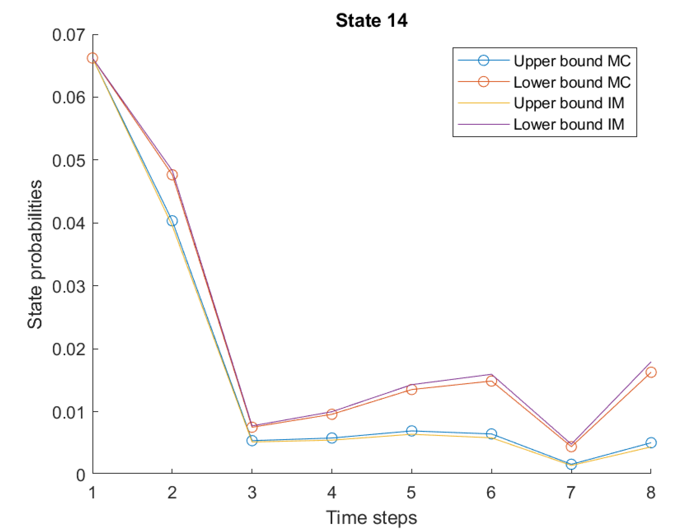
The maximum number of time steps should be chosen by inspecting each state over time. Indeed, different states might have a different propagation of the error over time: as shown in Figure 7 for state 14, the final interval is much narrower than state 2, hence it should not be chosen to predict the maximum number of time step required to maintain the desired level of accuracy.

Table 1. Lower and upper bounds of state probabilities at time step t = 8.

	LB	UB		LB	UB
$s_1$	0.192	0.678	$s_9$	0.047	0.175
$s_2$	0.051	0.217	$s_{10}$	0.015	0.053
$s_3$	0.049	0.224	$s_{11}$	0.013	0.05
$s_4$	0.018	0.063	$s_{12}$	0.003	0.016
$s_5$	0.062	0.250	$s_{13}$	0.023	0.051
$s_6$	0.023	0.077	$s_{14}$	0.005	0.021
$s_7$	0.017	0.081	$s_{15}$	0.003	0.019
$s_8$	0.005	0.025	$s_{16}$	0.001	0.006

shows the lower and upper bounds of state probabilities at time step $t=8$. The width of the uncertainty intervals is not uniform over the states, since it depends by the uncertainty assigned to the each element of the interval transition matrix. Among the states, state $s_1$ is the one that crosses the defined threshold at time step $t=8$.

In the scope of resilience-based analysis, using interval mathematics can help handling cases in which fault and repair rates are expected to change greatly and rapidly due to an external HILP event. In such a case, this tool would be necessary to take the necessary preventive, control and mitigating measures.

Furthermore, in case of resilience analysis, the conservatism is not a big concern such as in case of reliability studies, because the HILP events can cause enormous damage. Thus a faster, less accurate but more robust and conservative solution, can be accepted.

In this case, the results show that the system is more likely to be in state $s_1$, that corresponds to each component working properly: $s1=\{1,1,1,1\}$. However there are some states, such as $s_2,s_3,s_5$, whose probabilities’ upper bound has a non negligible value. Such states refer to the fault of a single component. The analysis suggests that the state $s_4$, corresponding to the single fault of the third element $s_4=\{1,1,0,1\}$ is much less probable than the other possible single faults. Operatively, this means that the system operator can focus on components other than the third, which appears to be robust. Finally, the state $s_9$, which is: $\{1,0,1,0\}$ also has a non-negligible upper bound probability, although the fault in this case is double. This result means that reinforcing strategies on components two and four are even more urgent.

4. Future Development

The analysis of the obtained results, and, in particular, the solution bounds reported in Figure 6, demonstrates as the performance of the proposed algorithm may degenerate in the presence of correlated uncertain sources. This phenomenon is mainly related to the inability of the interval-based operators in managing correlated uncertain variables. To face this issue, in this paper different mathematical operators aimed at computing reliable enclosures of the products between uncertain interval variables have been tested, and a novel product operator has been conceptualized. The main idea is to express each uncertain interval variable by an affine form $\widehat{x}$, which is a first order polynomial defined as follows:

$$\widehat{x}=x_0+x_1{ϵ}_1+x_2{ϵ}_2+\cdots +x_n{ϵ}_n,$$

(20)

where $x_0$, $[x_1\cdots x_n]$ and $[{ϵ}_1\cdots {ϵ}_n]\in [0,1]$ are the central value, the partial deviations and the noise symbols of the affine form $\widehat{x}$, respectively. The noise symbols are symbolic variables, which represent independent uncertainty sources affecting the uncertain variable x, and whose value is only known to be in the interval [−1 ,1] [38].

The connection between affine forms and interval variables is straightforward, once the radius of the affine form $R\left(\widehat{x}\right)$ is defined:

$$\begin{array}{c}\hfill x^I=[x_0-R\left(\widehat{x}\right),x_0+R\left(\widehat{x}\right)]\\ \hfill R\left(\widehat{x}\right)=\sum _{h=1}^n|x_i|.\end{array}$$

(21)

The multiplication between affine forms can be defined as:

$$\widehat{x}\ast \widehat{y}=x_0{y}_0+\sum _{h=1}^n(x_0{y}_h+y_0{x}_h){ϵ}_h+\sum _{h=1}^n\sum _{j=1}^n\left(x_h{y}_j\right){ϵ}_h{ϵ}_j.$$

This non-affine operation is traditionally approximated by bounding the second order terms:

$$\sum _{h=1}^n\sum _{j=1}^n\left(x_h{y}_j\right){ϵ}_h{ϵ}_j\le \sum _{h=1}^n|x_h|\sum _{j=1}^n|y_j|=R\left(\widehat{x}\right)R\left(\widehat{y}\right).$$

Starting from this result a new noise symbol describing the approximation error (i.e., endogenous uncertainty) can be defined as follows:

$$\widehat{x}\ast \widehat{y}=x_0{y}_0+\sum _{h=1}^n(x_0{y}_h+y_0{x}_h){ϵ}_h+R\left(\widehat{x}\right)R\left(\widehat{y}\right){ϵ}_{n+1}.$$

Unfortunately, the adoption of this operator seems inadequate in reliably solving the problem formalized in (16), since it lacks in describing the propagation of the approximation errors, and the number of noise symbols describing the endogenous uncertainty increases at each iteration. Hence, a new method for computing multiplication between affine forms is here proposed, which is based on the following robust formalization:

$$\widehat{x}\ast \widehat{y}=x_0{y}_0+\sum _{h=1}^n(x_0{y}_h+y_0{x}_h+x_h\sum _{j=1}^n\left(x_h{y}_j\right){ϵ}_j){ϵ}_h.$$

Compared to the traditional approach, this operator does not take into account the approximation error by introducing a new noise symbol, rather than spreading the corresponding endogenous uncertainty on the partial deviation of the primitive noise symbols, which are no longer numbers but affine forms. These variables, which are here referred as second order affine forms, can be properly managed in order to reliably solve the uncertain problem (16), considering all the possible combinations of the exogenous uncertainty, and the worst case instance of the approximation errors. The robustness of the computed solutions, which guarantee the rigorous inclusion of the real solution sets, is currently under investigation by the Authors.

5. Conclusions

Resilience-based planning must be integrated to reliability studies of power systems, in order to assure their security and robustness. Markov Chains can be an efficient tool to analyze power system’s reliability and resilience over time, however their accurate description requires a huge amount of data, that is not always present, especially in case of HILP events.

When studying the impact of HILP events, since there are not enough data available, transition matrices should not be defined as point values, but as intervals of uncertainty.

This paper employed interval Markov Chains to find robust bounds of the state probabilities over time. The validity of the method was assessed through Monte Carlo simulations. The results show that interval Markov Chains always result in outer bounds, enclosing all possible scenarios of the evolution of state probabilities. The conservatism of such bounds is related to the dependency between the uncertainty sources affecting the transition probabilities.

As the case study showed, incorporating uncertainties into resiliency planning tools can improve the confidence associated to the chosen mitigating actions. The results showed that an uncertainty of $10\%$ on the parameters affecting state transitions can lead to largely different state probabilities, which affect the calculation of risk and resiliency indices and the resulting mitigating actions.

Furthermore, the computational burden of this technique, compared to Monte Carlo, allows the simulation of large scale systems.

The future research direction, which is being explored by the authors, is the application of the described technique, enhanced by affine-based operators, to real world data-sets provided by transmission system operators.