Article

Mathematical Modelling and Operational Analysis of Combined Vertical–Horizontal Heat Exchanger for Shallow Geothermal Energy Application in Cooling Mode

1
Department of Mechanical Engineering, Universitas Syiah Kuala, Banda Aceh 23111, Indonesia
2
School of Mechanical Engineering, The University of Adelaide, Adelaide, SA 5005, Australia
*
Author to whom correspondence should be addressed.
Energies 2020, 13(24), 6598; https://doi.org/10.3390/en13246598
Submission received: 27 October 2020 / Revised: 10 December 2020 / Accepted: 11 December 2020 / Published: 14 December 2020
(This article belongs to the Special Issue Energy for Sustainable Future)

Abstract

:
Geothermal heat exchangers (GHEs) represent a buried pipe system, which can be utilised to harness renewable thermal energy stored in the ground to improve the efficiency of heating and cooling systems. Two basic arrangements of GHEs have been widely used: vertical and horizontal. Vertical GHEs generally have a better performance in comparison with the horizontal arrangement, and these systems are particularly suitable for confined spaces. Nevertheless, the main technical challenge associated with GHEs, for either the vertical or the horizontal arrangement, is the performance deterioration associated with an increase in the operation times during summer or winter seasons. In this paper, a combined horizontal-vertical GHE arrangement is proposed to address the current challenges. The combined GHE arrangement can be operated in five different modes, corresponding to different thermal loading conditions. These five operation modes of the combined GHE are analysed based on the transient finite difference models previously developed for the horizontal and vertical arrangements. The simulation results reveal that for the single operation mode (horizontal or vertical only), the vertical GHE performs better than the horizontal GHE due to relatively stable ground temperature deep down. While, for the combined operation mode, the series operations (horizontal to vertical or vertical to horizontal) of the GHE are superior to the split mode. It is found that the effect of the fluid mass flow rate ratio is trivial on the heat dissipation of the split mode GHE. The highest heat transfer rate in the split flow operational mode is rendered by the ratio of the mass flow rate of 40% horizontal and 60% vertical. In addition, the climate condition has more effect on GHE’s performance and the increase of the fluid flow rate it can enhance the amount of energy released by the GHE.

Graphical Abstract

1. Introduction

Increasing energy demands and crude oil depletion have forced the world to explore new energy resources, those that are not only sustainable but also have a minor environmental footprint. Shallow geothermal energy is one of the sustainable energy resources that could be applied to improve the efficiency of current and future heating and cooling systems. This renewable thermal energy is usually exploited in a geothermal heat exchanger (GHE); a system of pipes buried in the ground, in which the heat carrier fluid is circulated. GHEs are normally integrated with heat pumps and air conditioning systems. These systems use the ground as a heat source/sink during heating/cooling to provide the thermal comfort condition of buildings’ interiors in both winter and summer. Compared with the traditional air source heat pumps and air conditioning systems, the application of GHEs as a thermal energy rejecter/absorber can reduce energy consumption by 30%–60%, since the ground has a relatively stable temperature [1].
There have been two basic arrangements of GHEs: vertical and horizontal. Vertical GHEs have been widely installed in confined areas such as an urban area or an area where the earth is rocky close to the surface. The typical depth of vertical GHEs varies from 20 to 300 m [2]. Vertical GHEs have a better efficiency since the ground temperature at the deeper depth below the surface remains relatively largely constant all year around. The drawback of vertical GHEs, however, is their installation cost, which is higher than for the horizontal arrangement. In addition, the degradation in their thermal performance is relatively hard to recover because of the poor soil thermal conductivity and relatively deep depth of burring, which hinder the heat transfer rate to and from the atmosphere. Horizontal GHEs are mostly installed where a land area is available at low cost. They are buried in a horizontal trench, with a typical depth up to 2 m below the surface. The continuous thermal interaction between the ground and the atmosphere could improve the GHE’s performance through an appropriate operation mode. The diverse mechanisms of the heat transfer occurring on the ground surface could also facilitate the thermal recovery in the case of a horizontal arrangement.
The technical challenges associated with GHEs are their performance degradation with an increase in the operation time, which often happens in heating or cooling seasons. This performance degradation is slow to restore, especially for vertical GHEs. Meanwhile, it can be minimised if the GHEs are run intermittently or with a smaller thermal load, which can be achieved with the proposed GHE system, which combines both vertical and horizontal arrangements. To address the degradation performance problem caused by an imbalance in the heating and cooling loads, a number of researchers have proposed hybrid GHE systems and different operation strategies [3]. For example, hybrid GHE, solar energy systems, and heat pump have been suggested by a number of researchers [4,5,6,7,8], to cope with performance deterioration. Dai et al. [4] carried out an experimental study on a solar assisted ground source heat pump system. In the parallel mode, the performance of the heat pump, under three different flow rate ratios of working fluid inside both solar and shallow geothermal systems, is investigated. The outcomes of this study demonstrated that the hybrid systems could recover the degradation of soil temperature much faster than happens during natural recovery. In addition, the effect of the flow rate ratio in mode 4 has a significant impact on the electricity consumption. The electricity consumption decreases with the increase in the flow rate ratio of the solar heat storage water tank. Furthermore, mode 3 is recommended for use in the coldest months.
Kjellsson et al. [5] analysed different systems with a combination of a ground source heat pump and a solar collector to provide heating for houses and domestic hot water systems. The outcomes demonstrated that the system works in an optimal regime when the solar energy is utilised to recharge the borehole during winter time and to produce the domestic hot water during summer time. The performance of a solar assisted ground source heat pump, which is used for green house heating, was investigated by Ozgener et al. [6]. The archived exergetic efficiency of the overall system was reported to be at 67.7%. Yang et al. [7] presented a theoretical and experimental study on a solar-ground source heat pump system. The experimental coefficient of performances (COPs) of modes 2, 3, and 4 were obtained 2.69, 2.65, and 2.59, respectively. While the theoretical COPs were found to be 3.67, 3.64, and 3.52, which are quite different from the theoretical values. In addition, research on small ammonia heat pumps for space and hot tap water heater with a capacity of 8.4 kW to provide space heating and hot water has been done by Aleksandrs Zajacs et al. [8]. In this study, equation calculations have been carried out using the engineering equation solver (EES) to estimate the heat pump performance. The results of the calculations are able to provide electrical energy savings of up to 75% compared to using electric heating. The volume of the tank also affects the efficiency of the heat pump and compressor usage. The optimal tank volume is 1000 L to cover 2–3 h of high electricity price peaks.
Studies on hybrid ground source heat pump systems with a cooling tower as a supplemental heat rejecter were presented by a number of researchers [9,10,11,12,13]. Park et al. [9] proposed a new parallel system comprising of a hybrid ground source heat pump-cooling tower. The new parallel system enables the GHE to be switched off during the recovery period of the soil thermal condition. The performance of the heat pump was investigated at different flow rates of the fluid in the primary flow loop (the heat pump), GHE, and cooling tower. The results indicated that the parallel system of the ground source heat pump-cooling tower generates 21% COP more than that produced by the conventional ground source heat pump system. Man et al. [10] provided the technical and economic analysis of a hybrid cooling tower-ground source heat pump, based on the hourly load of a two storey residential building located in Hong Kong. The hybrid system in this study not only solves the thermal degradation problem, but also reduces the operation and capital costs of the air conditioning system. A study of the operation strategy of a hybrid cooling tower-ground source heat pump system was presented by Wang et al. [11]. The operation strategy consists of a fixed cooling set point, outside air reset, wet bulb reset, and load reset. Fan et al. [13] presented a theoretical design of a hybrid cooling tower-ground source heat pump, which takes into account the effect of borehole distance, borehole depth, and thermal properties of the grout. In this study, a combined strategy of operation was introduced. The results showed that the lowest energy consumption was obtained when the control strategies of the entering water temperature and wet-bulb temperature differences are combined.
Canelli et al. [14], presented an analysis of the energy, economic, and environmental performances of three different hybrid ground source heat pump systems including (1) a hybrid boiler-chiller-ground source heat pump, (2) a hybrid boiler-chiller-ground source heat pump and fuel cell, and (3) a hybrid boiler-chiller-ground source heat pump and photovoltaic thermal system. The system was optimised to meet the heating and cooling conditions of both residential and commercial buildings, which are in a sharing load. The results indicated that the hybrid system with the fuel cells and photovoltaic thermal system has a definite advantage in terms of energy savings, operational costs, and carbon emission reductions.
A detailed numerical study was conducted by Zhu et al. [15] to investigate the performance and economic characteristics of a combined vertical ground source heat pump and phase change material cooling storage system. The optimal performance of the hybrid system was achieved by varying the ratio of the phase change material cooling storage system to the total cooling load of the system. The obtained optimal cooling storage ratio was close to 40%.
A hybrid system of the ground source electrical heat pump and ground source absorption heat pump was proposed by Wu et al. [16]. The motivation for this study was to combine the features of both heat pumps, as the ground source electrical heat pump has higher energy efficiency in the cooling mode. Conversely, the ground source absorption heat pump has higher energy efficiency in the heating mode. This study also presented the effects of supply ratios on thermal imbalance ratios, annual primary energy efficiency, and cost-efficiency characteristics.
A theoretical study on a hybrid air source heat compensator-vertical ground source heat pump system was conducted by You et al. [17], using a simulation tool, TRNSYS. Four operation strategies were analysed including an air source heat compensator for direct heat compensation, a combined air source heat compensator-ground source heat pump for heat compensation, a combined air source heat compensator-ground source heat pump for space heating, and an air source heat compensator-ground source heat pump for domestic hot water. The results showed that the hybrid air source heat compensator-ground source heat pump reduces energy consumption by 23.86% compared with the boiler-split air conditioner system. Additionally, the operational costs are reduced by 50%. Another study has done by Xianting Li et al. [18] by developing an energy-efficient heat pump system using the TRNSYS simulation tool in a combination of a hybrid source and three types of hybrid source heat pumps to calculate the efficiency of year-round operation. The results show that the hybrid heat pump system can maintain heat reliability during year-round operation including winter. This hybrid source heat pump system saves energy up to 15% and the payback period is approximately five years. In addition, Gaoyang Hou et al. [19] also conducted a simulation using the TRNSYS tool to analyse the work system of heat pumps sourced from hybrid soil with optimal control strategies. His research combines a horizontal ground loop and a liquid dry cooler with a short and long term simulation process on TRNSYS to analyse soil thermal conditions and energy variations. Gaoyang Hou et al. also performed a simulation using the TRNSYS tool to analyse the heat pump working system sourced from hybrid soil with optimal control strategies. Their research combines a horizontal ground loop and a liquid dry cooler with a short and long term simulation process on TRNSYS to analyse soil thermal conditions and energy variations. The simulation results show that the overall performance in the short-term simulation is influenced mainly by the temperature of the diverter heating set rather than by cooling. Diverter heating set was recommended about 8–10 °C in climatic zones similar to the Birmingham area by combining long-term coefficient of performance (COP) values and soil thermal variation.
A hybrid active air source regeneration-ground source heat pump system was studied by Allaerts et al. [20]. In this study, the borehole area is divided into two different regions, namely warm and cold regions. These two different regions were proposed to balance the extraction/rejection of heat during heating and cooling periods. In addition, a supplementary dry cooler was used to capture heat/cold during summer/winter to recover the degradation of the soil thermal condition. According to Allaerts et al. the proposed hybrid system can significantly reduce the size of the borehole area by up to 47% in the cost-optimal configuration.
The brief review of the literature [1,2,3,4,5,6,7,8,9,10,11,12,13,14,15,16,17,18,19,20,21,22] above shows that most researchers proposed a hybrid cooling tower-ground source heat pump for a cooling load dominated regime and a hybrid solar system-ground source heat pump for heating load dominated conditions. Some other studies proposed a combined system of a ground source heat pump with different additional heat rejecter/absorber systems including a boiler, chiller, fuel cell, photovoltaic, and phase change material cooling storage systems. Additionally, a ground source heat pump system with two different regions of BHEs including warm and cold was recently suggested and analysed. However, it seems a comprehensive study of a combined GHE arrangement with different operation modes has yet to be presented.
This paper is focused on the operational analysis of a combined horizontal-vertical GHE to address various demands and thermal loading conditions. The performance of the combined GHE is studied based on the results of a transient finite difference model developed in this paper. The effects of continuous and intermittent operation conditions, climate condition and fluid mass flow rate on the GHE’s performance are investigated with this new model. Based on the analysis of the outcomes of numerical simulations, the recommendations for the optimum operation of combined GHEs are summarised in the conclusion.

2. Development of a Combined Horizontal–Vertical Geothermal Heat Exchanger Model
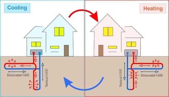
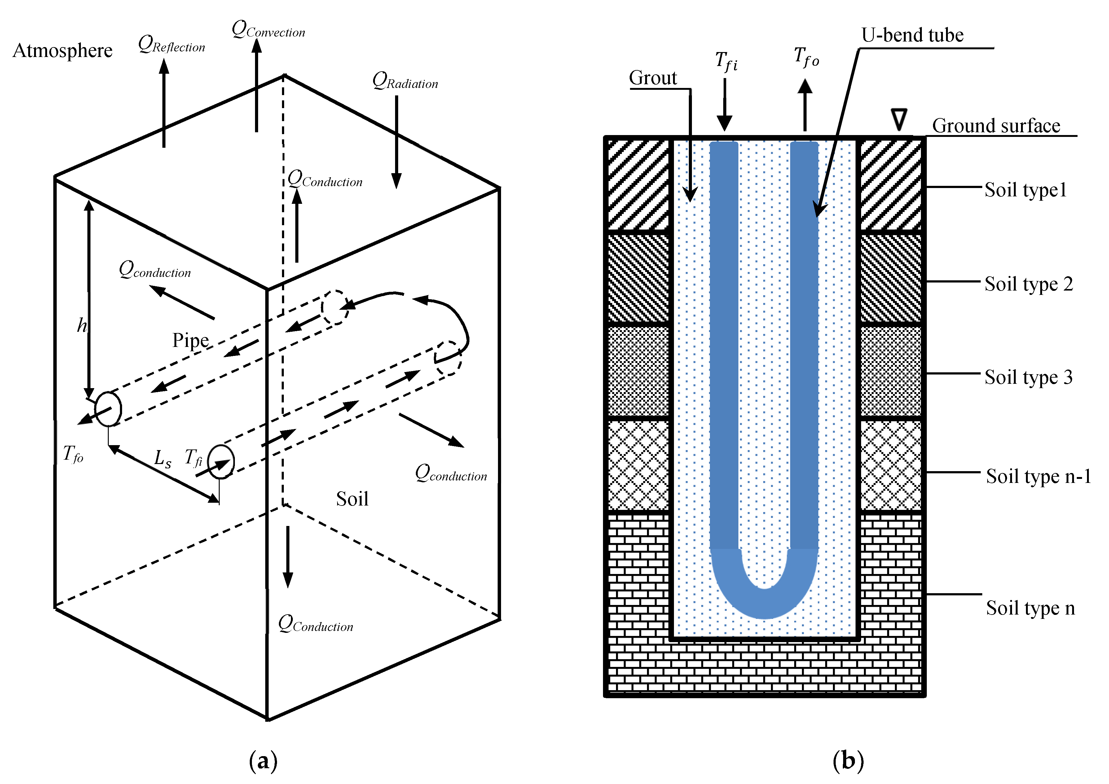
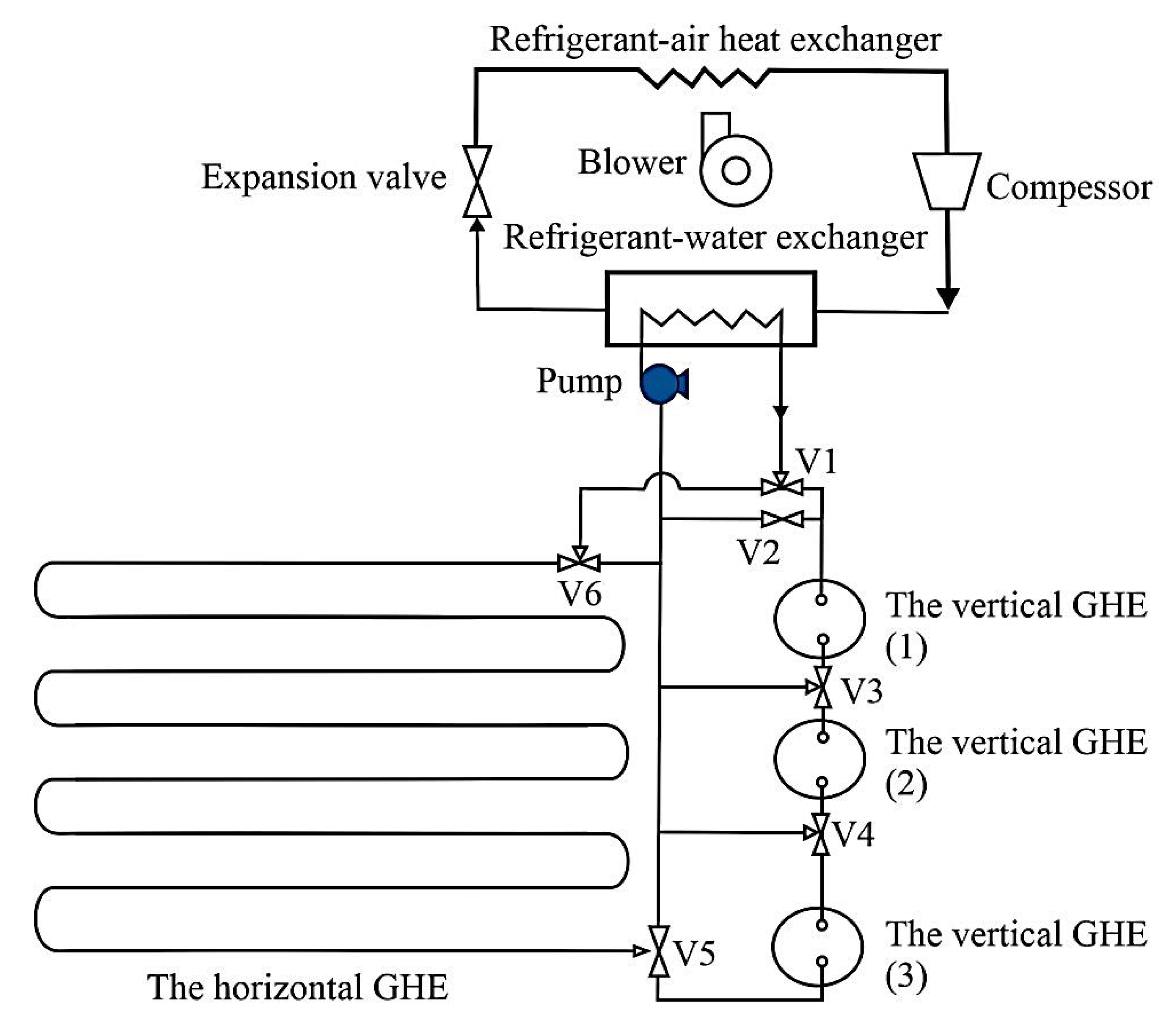
2.1. Physical Model

The physical model is described first including a number of simplifications, which are usually needed for quantitative analysis of complex systems or phenomena. A horizontal GHE, as shown in Figure 1a, represents a multi-U-shaped pipe buried in a trench at a specific depth h close to the ground surface. A horizontal GHE has a total length L, diameter d, wall thickness t, and pipe spacing L s . The heat transfer process at the horizontal GHE occurs when the fluid at a temperature Tfi enters the GHE and exchanges the heat energy with the pipe’s inner surface by convection. The heat then conducts through the pipe wall to the surrounding soil. The ground exchanges the heat at the ground surface with the atmosphere through diverse heat transfer mechanisms including reflection, convection, radiation, and evaporation. A vertical GHE, as shown in Figure 1b, could be modelled as a single U-shaped pipe, which is buried inside a borehole having a diameter Db and depth z. The pipe is described by diameter d, length L, thickness t, and shank spacing L s . The borehole is usually filled with a material, which has a relatively higher thermal conductivity than the surrounding soil, in order to enhance the GHE’s thermal performance. The borehole could be confined by different types of soil/rock layers that have different thermal conductivities. The heat transfer at GHE occurs when the fluid is operating at a temperature of Tfi and the mass flow rate m is circulated through a U-shaped pipe, exchanges its heat with the pipe’s wall by convection. The heat then flows through the pipe’s wall, grout, and surrounding soil by conduction sequentially. The convection occurs when the soil surface exchanges the heat with the atmosphere. As mentioned above, a vertical GHE is appropriate for installation in areas with limited land access. It may benefit from the relatively stable ground temperature at the deeper ground depth, and it leads to an improvement in performance. However, this performance decreases with the increase in the operation time, and it may take a season to recover fully. The poor soil conductivity and relatively deep depth of burring are the main reasons for the slow recovery of the soil temperature.
To take advantage of different arrangements and negate their disadvantages, a combined, structured, horizontal–vertical GHE was proposed, see Figure 2. This figure represents a schematic diagram of the proposed combined horizontal–vertical GHE, coupled with a heat pump. The hybrid horizontal vertical GHE can be operated in five different modes through the adjustment of the valves, namely (1) the horizontal GHE only, (2) the vertical GHE only, (3) the horizontal to the vertical GHE, (4) the vertical to the horizontal GHE, and (5) both the horizontal and the vertical GHEs concurrently, by splitting the fluid flow.

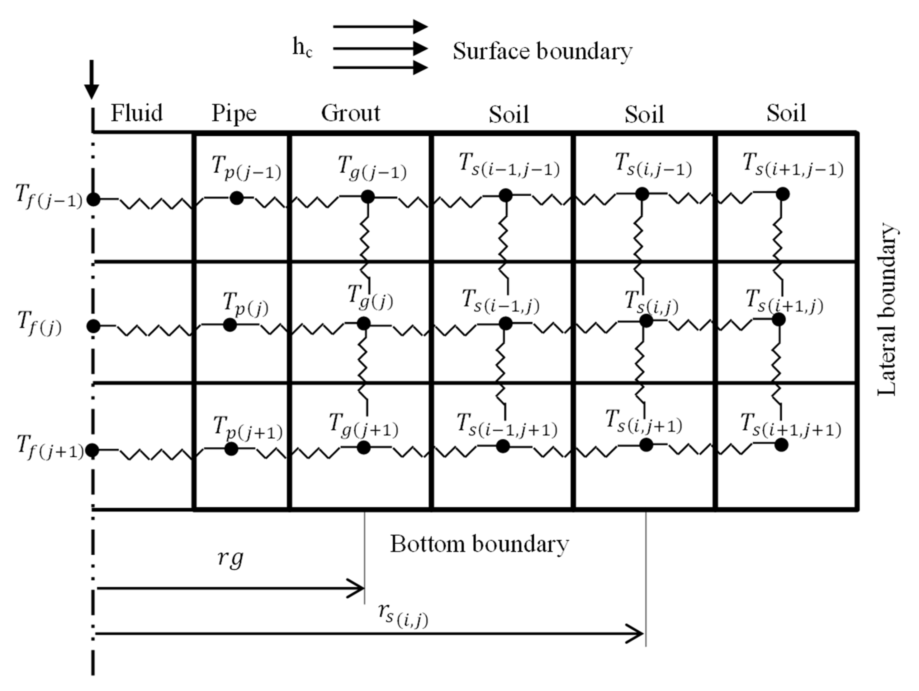
2.2. Mathematical Model

The performance of the combined GHE was studied based on the previously developed mathematical models for the horizontal [21] and vertical [22] GHE, respectively. The key equations in these models are briefly summarised below.

2.2.1. Governing Equation of the Soil

The thermal model of the soil domain around the horizontal GHE is developed based on the Cartesian coordinates as it is easy to handle when applying the soil’s internal source term, in which the value varies with the increase in the soil depth. The governing equation of the soil domain around the horizontal GHE is given as:
1 α s T s t = 2 T s x 2 + 2 T s y 2 + H s k s
The thermal model of the soil domain around the vertical GHE is developed by considering the cylindrical coordinates. The cylindrical coordinates are selected because these represent the shape of the borehole, thus the boundary conditions can be easily defined and prescribed. As a result, an accurate result can be obtained. The governing equation of the soil domain around the vertical GHE is given as
1 α s T s t = 2 T s r 2 + 1 r T s r + 2 T s z 2 + H s k s
An internal heat source term was used to take into account the effect of seasonal changes in soil temperature [21,23], expressed by the following equation:
H s = ρ s c s Δ T s Δ t
The direct measurement or analytical approach can be used to determine deviations in soil temperature during the process of seasonal change. The experimental results are preferred as they represent the actual soil temperature. However, it is sometimes hard to obtain the measurement data, especially for a specific location and a certain depth. Thus, the analytical equation presented by Baggs [24] was used in this work:
T ( x , t ) = ( T m ± Δ T m ) + 1.07 k v A s e ( 0.00316 x ( 1 α ) 0.5 ) c o s [ 2 π 365 ( t t 0 0.1834 x ( 1 α ) 0.5 ) ]

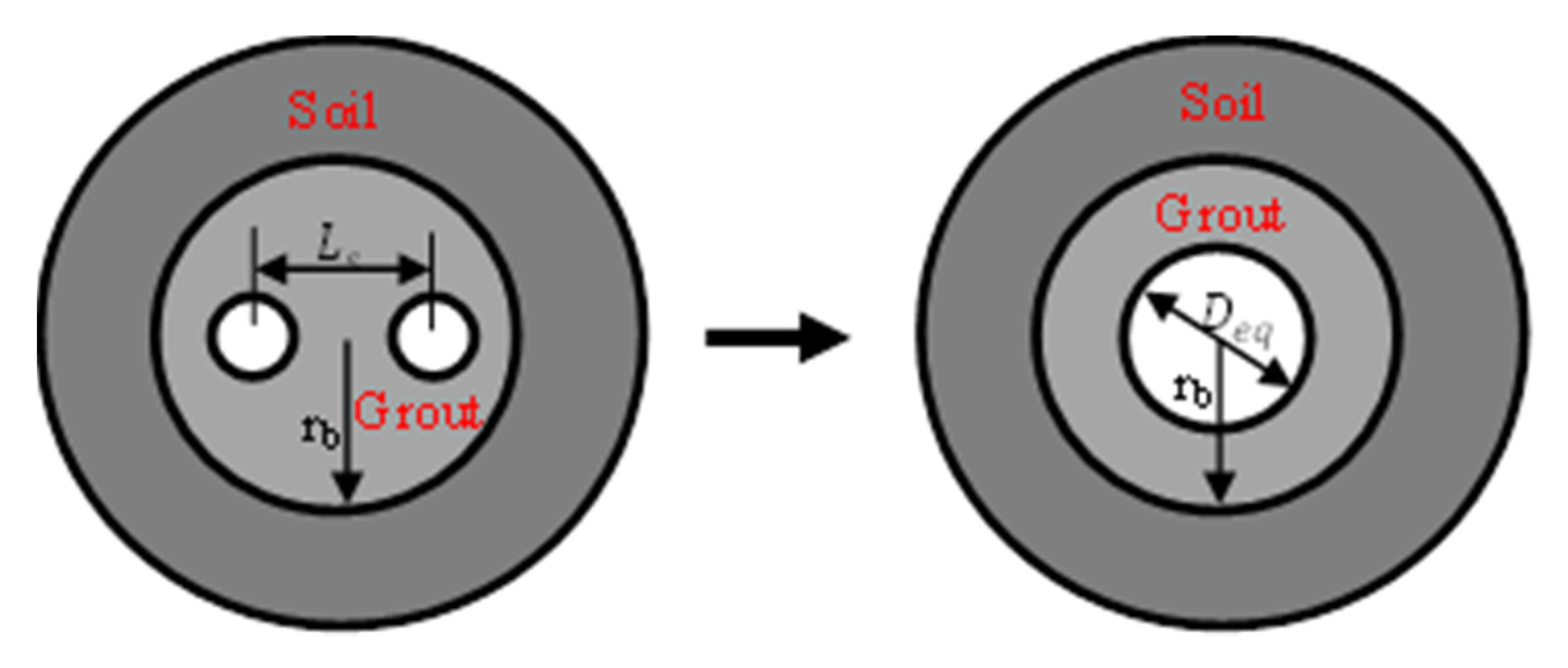
2.2.2. Governing Equation of the Temperature Exchange in the Grout for the Vertical GHE

The governing equation of the grout is given by a similar equation to the one above:
1 α g T g t = 2 T g r 2 + 1 r T g r + 2 T g z 2

2.2.3. Governing Equation of the Pipe

The energy balance equation for the pipe is
c p ρ p V p T p t = A h f ( T f T p ) + k g A 0.5 Δ r ( T s T p )
The area of the pipe for the vertical GHE was determined based on an equivalent pipe diameter, which is given later by Equation (8).

2.2.4. Governing Equation of the Fluid

For the working fluid, the energy balance equation states
c f ρ f A T f t = π d i n h f ( T p T f ) m ˙ f c f T f z
Equation (6) can be applied directly to the evaluation of performance of horizontal GHE. While for the vertical GHE, the internal pipe diameter d i n was replaced with an equivalent pipe diameter D e q since the single U shaped pipe is represented as a pipe, which has an equivalent diameter (refer to Figure 3). The equation to calculate the equivalent diameter has been developed and validated by Gu and Oneal [25] as:
D e q = 2 D p L s
The equation is valid if D p L s r b

2.2.5. The Initial and Boundary Conditions

  • The initial conditions are:
    T s = T   ( x , t ) ,   t = 0
    T g = T s ,   t = 0
  • The boundary conditions of the computational domain of the horizontal GHE are:
    T s x   | x = 0 = 0
    T s x   | x = x m a x = 0
    Q c a , y = 0
    T s y   | y = y m a x = 0
  • The boundary conditions of the computational domain of the vertical GHE are:
    Q c f , r = r i n
    T s r   | r = r m a x = 0
    Q c a , z = 0
    T s z   | z = z m a x = 0
The system of differential Equations (1), (2), and (4)–(6) were solved by using an explicit finite difference scheme, which provided the accurate solution for the temperature distribution in the soil, grout, pipe, and fluid. As an example, Figure 4 shows the computational domain of the vertical GHE. The working fluid exchanges the heat energy with the pipe’s surface, which then flows through the pipe wall in a 1D way. The heat is then transferred through the grout and surrounding soil in a 2D manner. Two different boundary conditions are applied at the boundary of the soil domain. The convection heat transfer is considered at the ground surface, while the adiabatic conditions are applied at the bottom and lateral edges of soil domain boundaries.
To achieve the stability of the explicit numerical calculations, the time step Δ t must be within the Courant–Friedrichs–Lewy stability range [26], which is given by:
| ψ | 1 ,   Δ t Δ z v f
Total of heat exchange by the GHE was calculated in accordance with the following equation:
Q = m ˙ c p ( T f i T f o ) Δ t
For the split flow mode, the final temperature of mixed fluid from both the horizontal and the vertical GHE was found as:
T f m i x = ( m ˙ f h   c f   T f o h +   m ˙ f v   c f   T f o v ) ( m ˙ f h   c f +   m ˙ f v   c f )
The described GHE’s models were validated against the experimental data [21,22,23] and will be used to simulate the performance of a combined GHE.

3. A Hypothetical Case Study

In this study, each arrangement of the GHEs (horizontal or vertical) was set to have the same parameters including the pipe length, pipe diameter, and fluid flow rates. The soil domain around the GHEs was assumed to be a single soil layer, which was homogeneous and isotropic. Table 1 presents the parameters of the reference case used in the simulation to be described next.
The initial temperature of the ground was estimated using the analytical equation (4) suggested by Baggs [24]. The Baggs’ equation was determined based on the input parameters of the climate conditions data. The amplitude data for annual air temperature and the average air temperature was obtained from the Australian Bureau of Meteorology [29]. The variable ground temperature for the local site was based on the data given by Baggs [24]. Table 2 summarises the parameters of the reference used to estimate the soil temperature conditions. Figure 5 shows the typical changes of soil temperatures in Adelaide and Brisbane at the end of winter (in August) and summer (in February). As observed from the figure that the soil temperature in Adelaide was lower than in the Brisbane. This tendency could be affected by mild, and generally a warm and temperate climate of Adelaide compared to humid subtropical climate of Brisbane as represented by the parameter of average annual air temperature ( T m ) in Equation (11). Besides the local site variable of the ground temperature ( Δ T m ), which varied with geographic location, it also affects the soil temperature. As an example, Figure 6 shows the ambient temperature in Adelaide and Brisbane on three consecutive summer days. These were used in the case study. In general, it can be seen from the figure that the pattern of air temperature was almost the same. The profile of air temperature fluctuated during day and night. For these three randomly selected summer days it was found that the air temperature in Adelaide was slightly higher than that in Brisbane.
The effect of seasonal changes on the soil temperature is modelled by incorporating the internal source term concept into the GHE model [21]. The value of the internal source term varied with the soil depths. It was higher in a shallow region and lower in a deeper zone. At a depth of 12 m below the ground surface, the value of the internal source term was assumed to be zero (this corresponded to the depth at which the effect of the ambient temperature on the soil temperature was negligible). Figure 7 shows the absolute value of the internal source term at various depths for two reference locations, namely Adelaide and Brisbane. As is shown in Figure 7, at the upper layer (0–3.5 m depth), the internal source term of the soil in Brisbane was relatively higher than in Adelaide. However, at a deeper layer, the condition was in the opposite. This phenomenon could be affected by meteorological, terrain, and subsurface conditions. The value of the internal heat source was positive when the ground temperature was warm (August to February) and conversely it was negative when the ground temperature was cool (February to August), as is shown in Figure 5.

4. Results and Discussion

This section shows the simulation outcomes of the GHE subjected to five operational modes, as described above. The analysis and discussion on continuous operation, intermittent operation, split flow operation, climate condition, and variations of the fluid mass flow rate will be discussed in the following section.

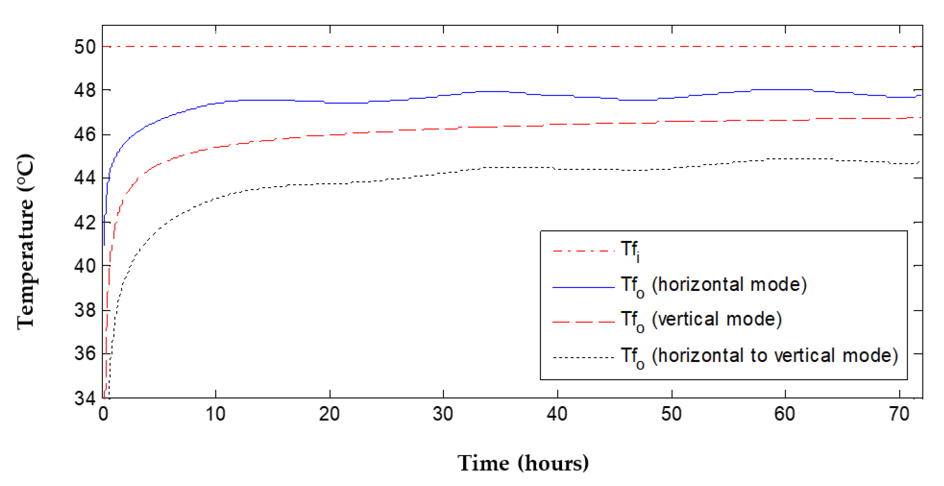
4.1. Continuous Operation

Figure 8 shows the simulation results of the GHE, which was operated on three consecutive summer days, with respect to the geological and climate conditions corresponding to Adelaide (South Australia). The amount of energy released by the GHE was calculated using Equation (21). It is observed that the lowest value of the outlet fluid temperature could be attained so the highest amount of energy can be released. As an example, Figure 9 provides the profile of the fluid temperature generated by operation of the horizontal, vertical, and the horizontal to the vertical GHE. This figure demonstrated that the outlet fluid temperature increased with the increase in the operation period. The accumulation of heat in the surrounding soil during the operation of the GHE led to a reduction in the heat transfer rate. As is shown in the Figure 9, the profile of the outlet fluid temperature of the vertical GHE was relatively stable when compared with those generated by the horizontal and the series operation modes. This phenomenon occurred because the ambient temperature, which fluctuated diurnally, did not have a significant effect on the performance of the vertical GHE. From Figure 8, it followed that the lowest energy was released when operating the horizontal GHE only. The horizontal GHE released 1002 kW less energy than that released in 3 days by the vertical GHE. The relatively stable temperature of the ground at a deeper layer might enhance the heat transfer capacity of the vertical GHE and led to better thermal performance. The amount of energy released could be increased by using the combined operation mode of the GHE, including the split flow and series operation modes. It can be seen that the series operation mode, from horizontal to vertical, could release slightly higher energy, namely 22 MJ more than the opposite operation mode. While the split flow mode, with a ratio of fluid flow at 50% in the horizontal GHE and 50% in the vertical GHE, released less energy than the series operation mode. The average heat transfer rate was calculated by dividing the amount of energy released with the operation period, namely 72 h. The single arrangement of the horizontal or the vertical GHE generated an average heat transfer rate of 6.3 kW and 10.2 kW, respectively. The combined arrangements produced a relatively higher heat transfer rate namely: 15.7 kW, 15.6 kW, and 15.4 kW for operation modes from the horizontal to the vertical, from the vertical to the horizontal GHE, and by splitting the fluid flow, respectively. Therefore, the horizontal or vertical GHE may be operated when the loading load was relatively low. At peak loads or when heating/cooling demands were relatively high, the combined GHE’s operation could have a significant advantage, see Figure 8.

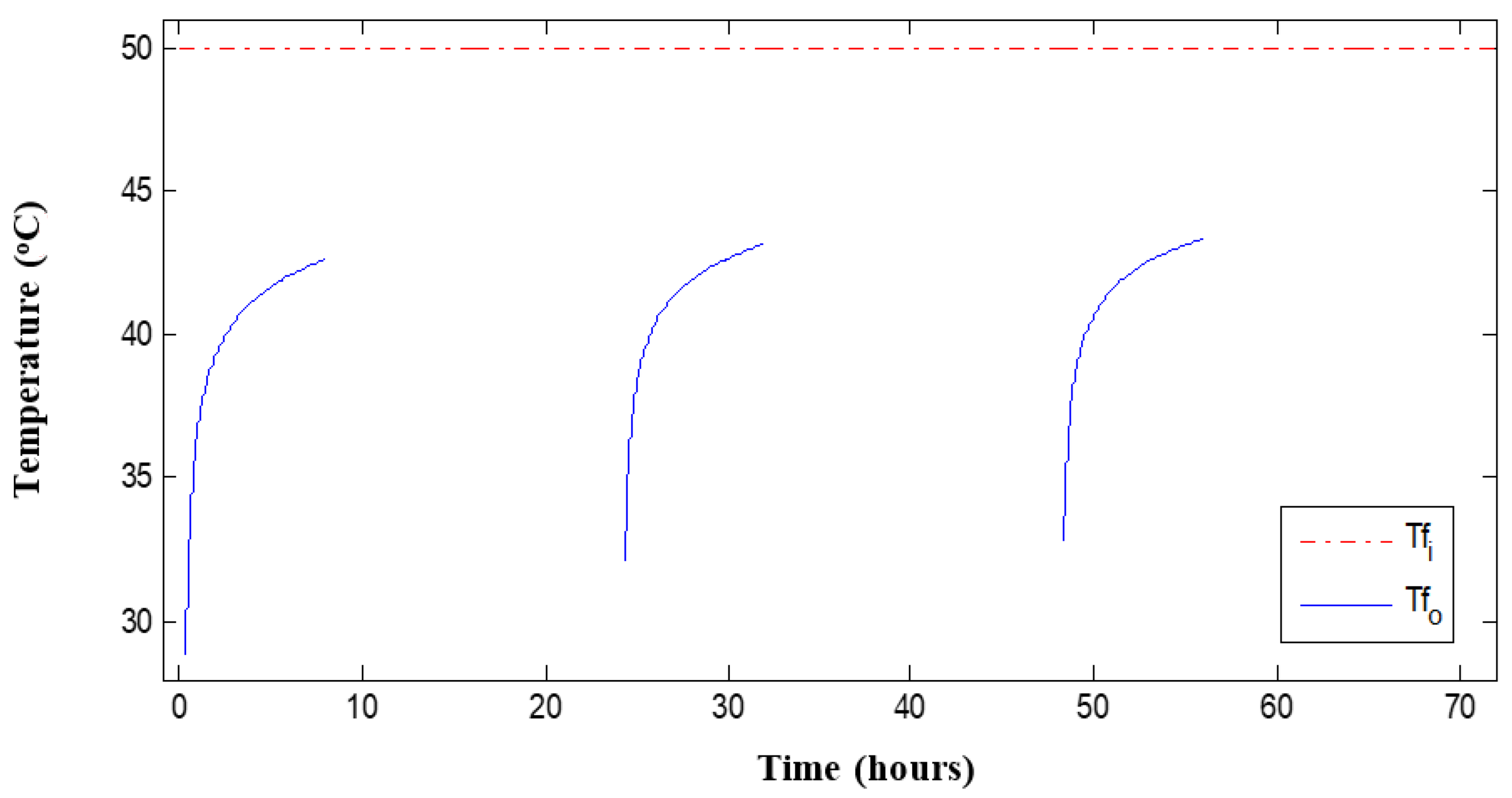
4.2. Intermittent Operation

The GHE can also be operated in the intermittent condition to cope with cyclic load conditions. Figure 10 shows the amount of energy released by the GHE operating intermittently in three summer days, see Figure 5 and Figure 6. The GHE ran for 8 h (during the working hours) and was off for 16 h daily. The results display that during 24 h of operation, the horizontal GHE released 41% less energy than the vertical GHE. The combined operation modes of the GHE could increase the amount of energy released, as the contact area, where heat was exchanged with the surrounding soil, increased. It is seen that the series operations could release 40.8% and 39.6% more energy than the vertical mode, for the horizontal to vertical and vice versa modes, respectively. In the split flow mode, the fluid is split to flow with a ratio of 50% in the horizontal GHE and 50% in the vertical GHE. The results demonstrate that the split flow mode released 2.8% less energy than the horizontal to vertical mode. Even though, the amount of energy released in the intermittent operation regime was less than that generated by the continuous operation due to the total operation period in the intermittent condition was less compared with the continuous condition. However, the average heat transfer rates increased. They were 60.1% for the horizontal mode, 68.5% for the vertical mode, 54% for the horizontal to vertical mode, 53.5% for the vertical to horizontal mode, and 52.6% for the split flow mode. In the intermittent operation condition, the deterioration of the ground temperature during the operation hours is possible to recover during the time when the system is switched off. As a result, it increases the heat transfer rate of the GHE and produces lower outlet fluid temperature over the next day’s operation as reflected by an example of fluid temperature generated by the vertical to horizontal mode (see Figure 11).

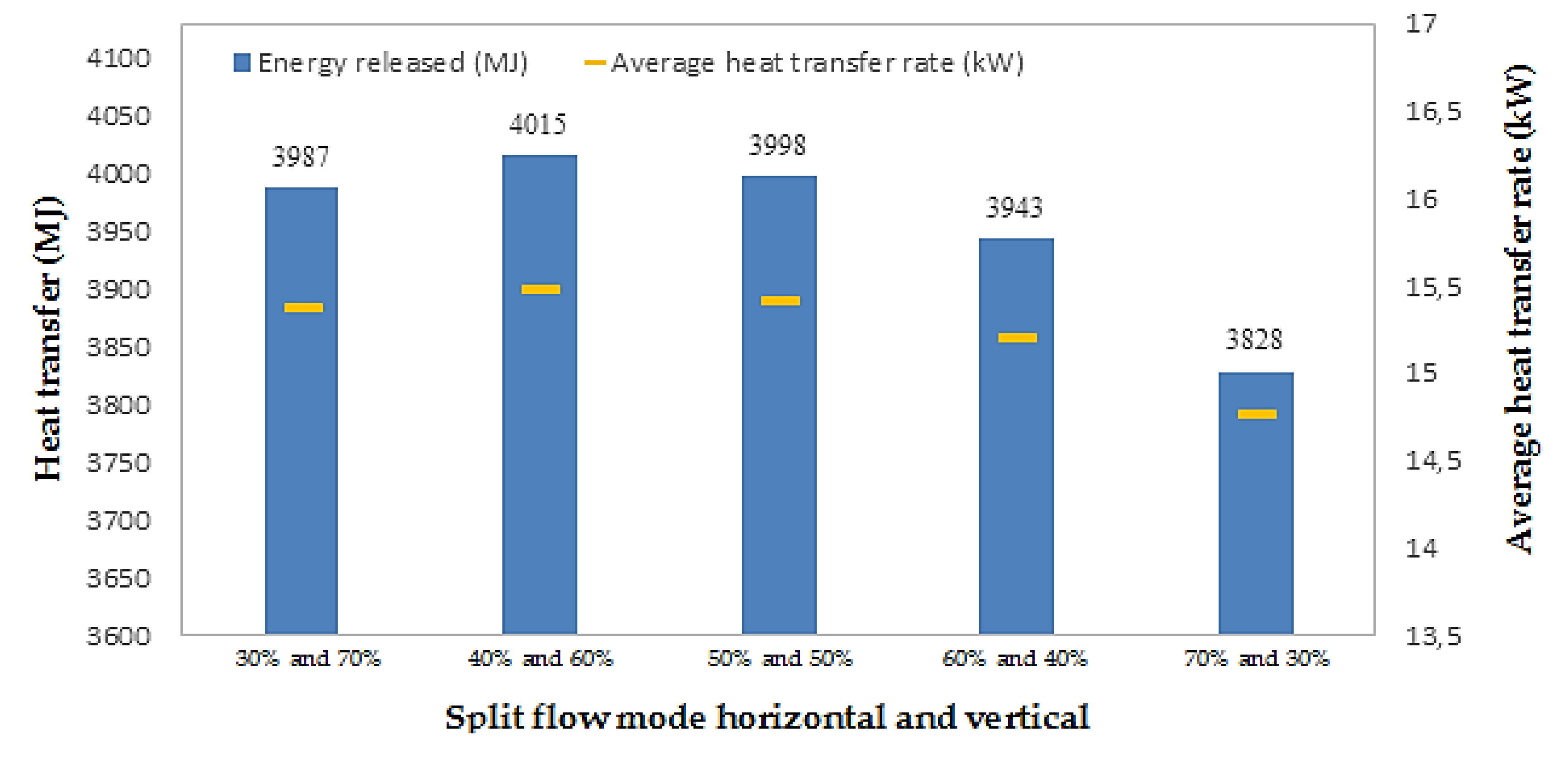
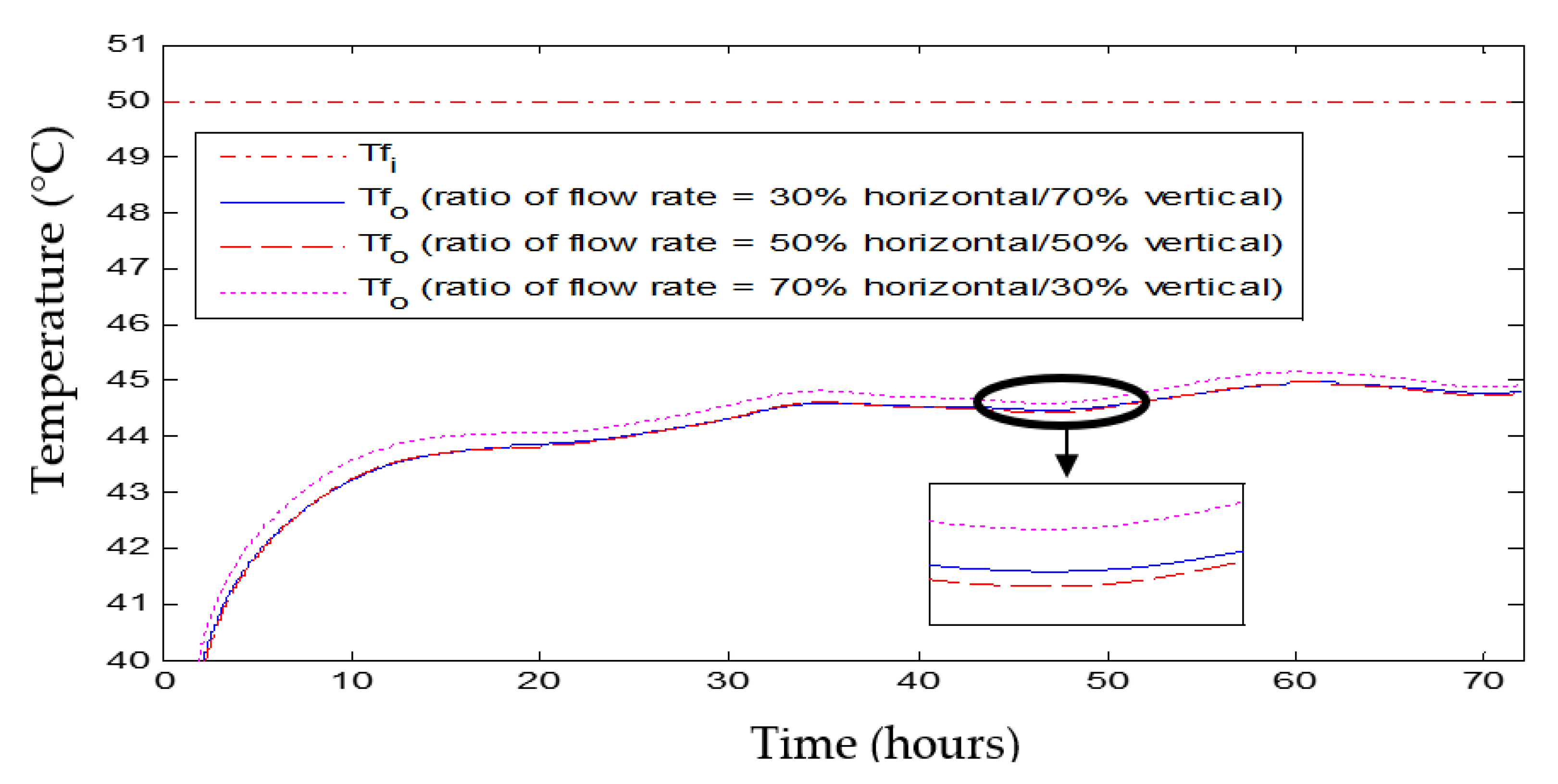
4.3. Split Flow Operation

In this section, the effect of the fluid mass flow rate ratio in the split flow operation mode was investigated. The ratio of the fluid mass flow rate varied as follows: 30%:70%; 40%:60%; 50%:50%; 60%:40%; and 70%:30% for the horizontal and the vertical GHE, respectively. From the current numerical simulations, it was found that the ratio of fluid mass flow rate in the split flow mode did not significantly affect the amount of energy released by the GHE, as shown in Figure 12. As an example, Figure 13, presents the outlet fluid temperature of the GHE at three different flow rate ratios, namely: 30%:70%; 50%:50%; and 70%:30% for the horizontal and the vertical GHE, respectively. It is found that the difference in the outlet fluid temperature was relatively small. The highest fluid outlet temperature was yielded by the GHE with a flow rate ratio of 70%:30%. It can be seen that the GHE operated with a flow rate ratio of 70% horizontal and 30% vertical released the lowest amount of energy across three consecutive days of operation, namely, 3% less than the one with a flow rate ratio of 60% horizontal and 40% vertical. The amount of energy released gradually increased with the increase of the ratio of the fluid mass flow rate in the vertical GHE and declined at the ratio of 30% horizontal and 70% vertical GHE namely, 0.7% less than that with a ratio of 40% horizontal and 60% vertical GHE. This tendency was due to a significant reduction in the fluid mass flow rate in the horizontal GHE (only 30% of the total fluid flow rate). At a lower mass flow rate, the thermal resistance of the horizontal GHE increased as a reduction in fluid mass flow rate was directly proportional to the decrease in the convective heat transfer coefficient between the working fluid and the inner pipe surface. As a result, it decreased the heat transfer rate of the horizontal GHE. In addition, with 70% of mass flow rate in the vertical GHE, the surrounding soil temperature deteriorated quickly due to heat accumulation, leading to degradation in the heat transfer capacity of the vertical GHE. From the Figure 12, it can be seen that the highest heat transfer rate was produced by the GHE with a ratio of flow rate of 40% horizontal and 60% vertical namely, 15,490 kW.

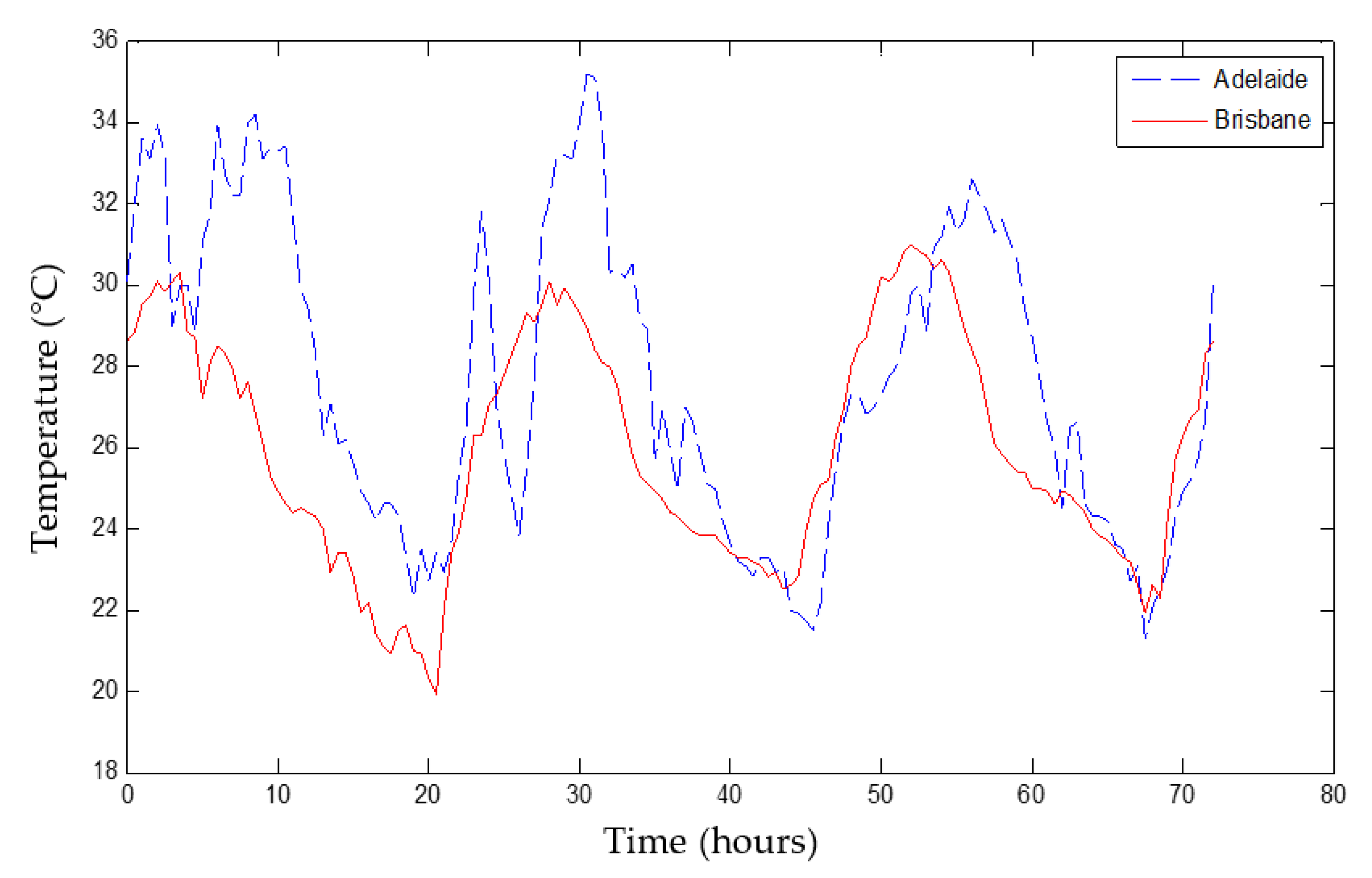
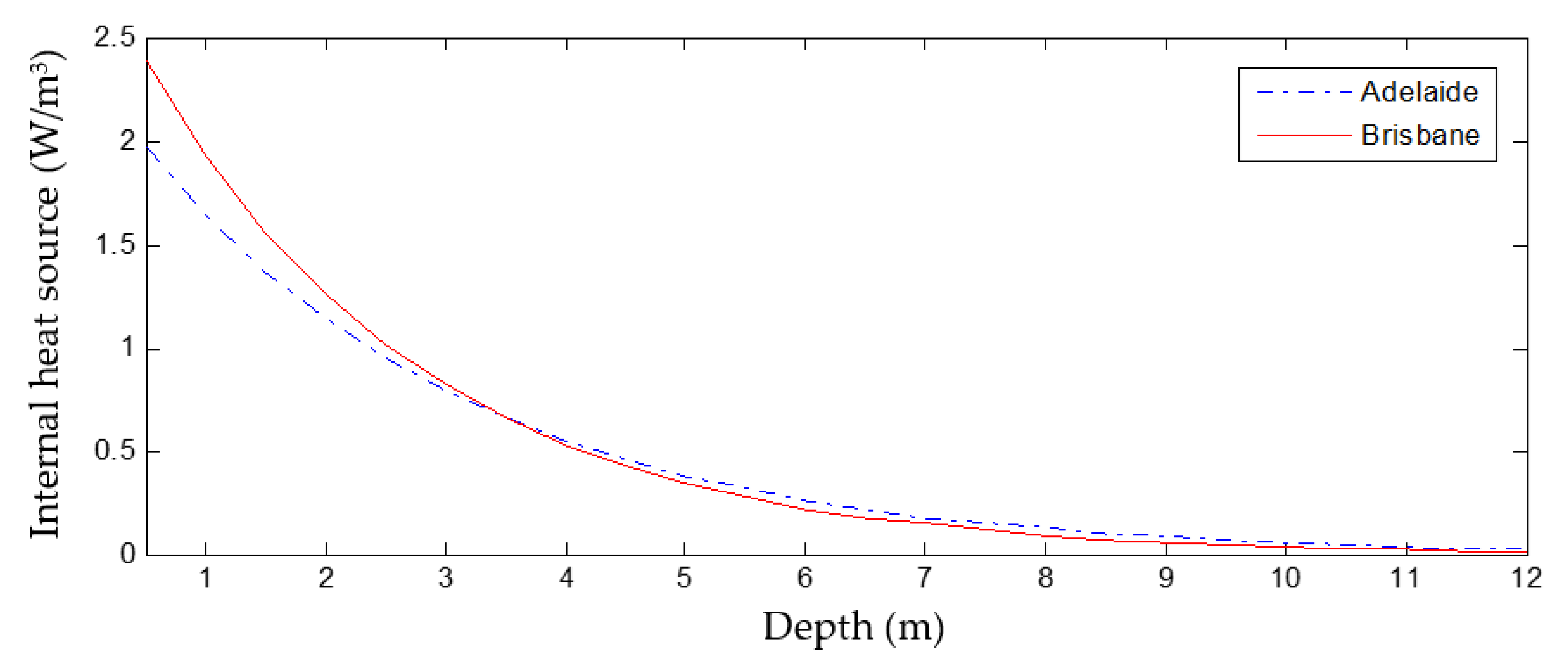
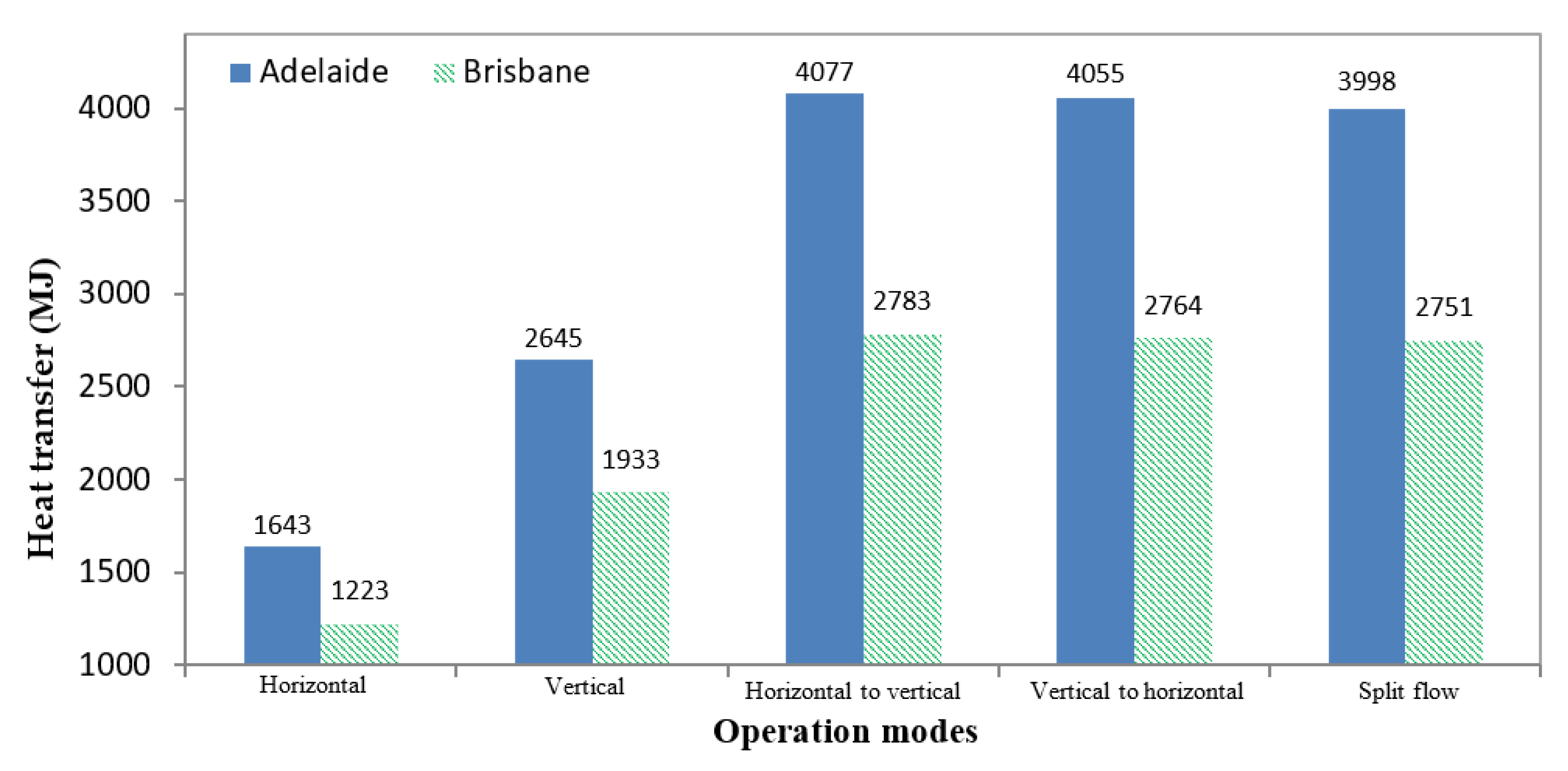
4.4. Climate Condition

The performance of the GHE installed in a temperate climate corresponding to Adelaide was compared with that installed in a subtropical climate, such as near Brisbane. Figure 14 summarises the performance of the GHE, which was installed in two different regions, with different climate conditions. It was found that during 72 h (3 days: 10–12 January) of the continuous operation, the GHE installed in Adelaide’s temperate climate could release 34.3% and 26.9% more energy compared with that installed in Brisbane, for the horizontal and vertical mode, respectively. While for the combined modes including horizontal to vertical, vertical to horizontal, and split flow were 31.7%, 31.8%, and 31% higher, respectively. It is observed that operating the vertical GHE only, in the temperate climate, Adelaide, could release an amount of energy that was almost the same as that released by the combined operation mode, in the subtropical climate. This tendency occurred because the climate condition influenced the initial soil temperature in both regions. The initial soil temperature in Adelaide was lower than that in Brisbane, as seen in Figure 5. In addition, the difference in soil types in both locations contributed to the heat transfer capacity of the GHE. As a result, the GHE installed in a temperate climate, Adelaide, produced a lower outlet fluid temperature as demonstrated in Figure 15.

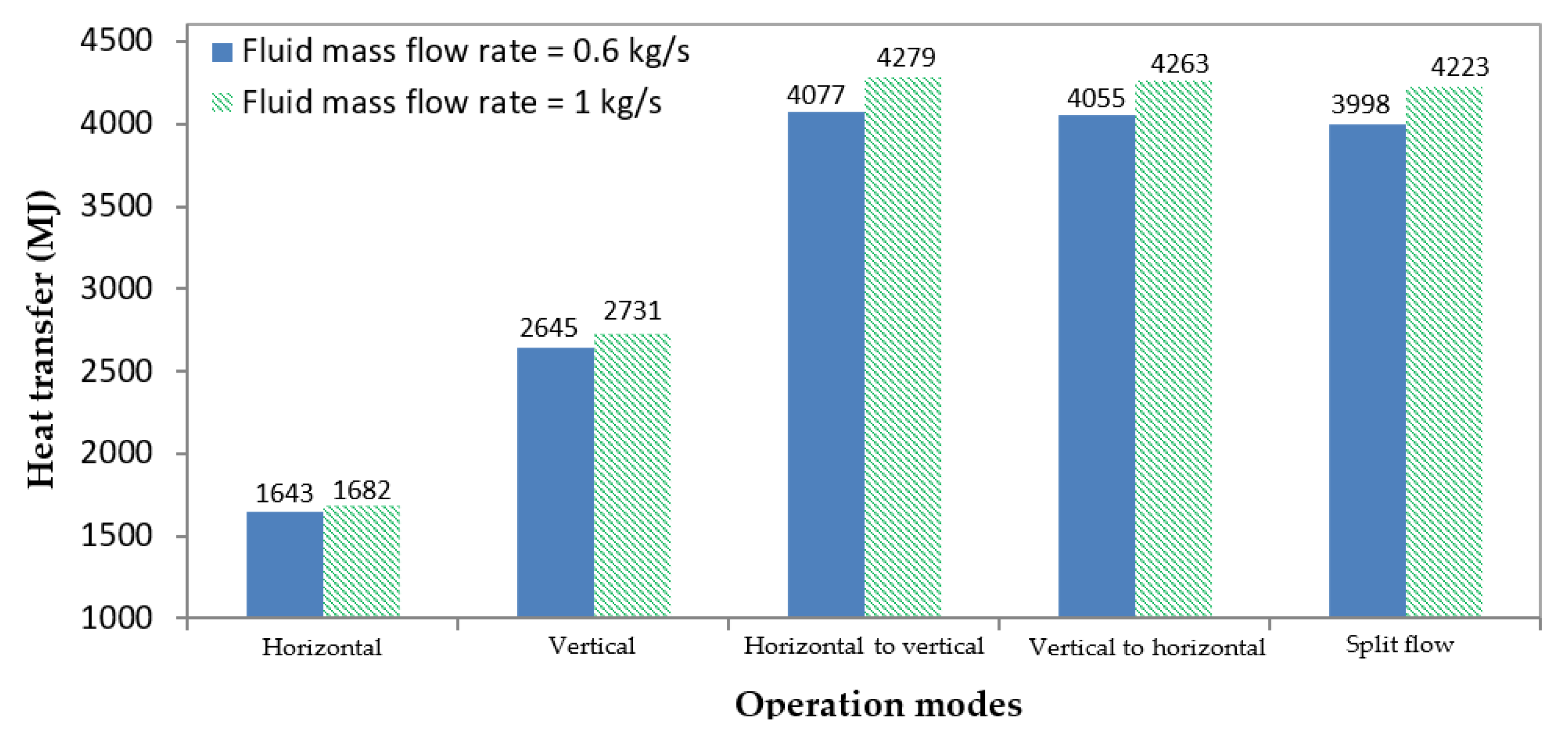
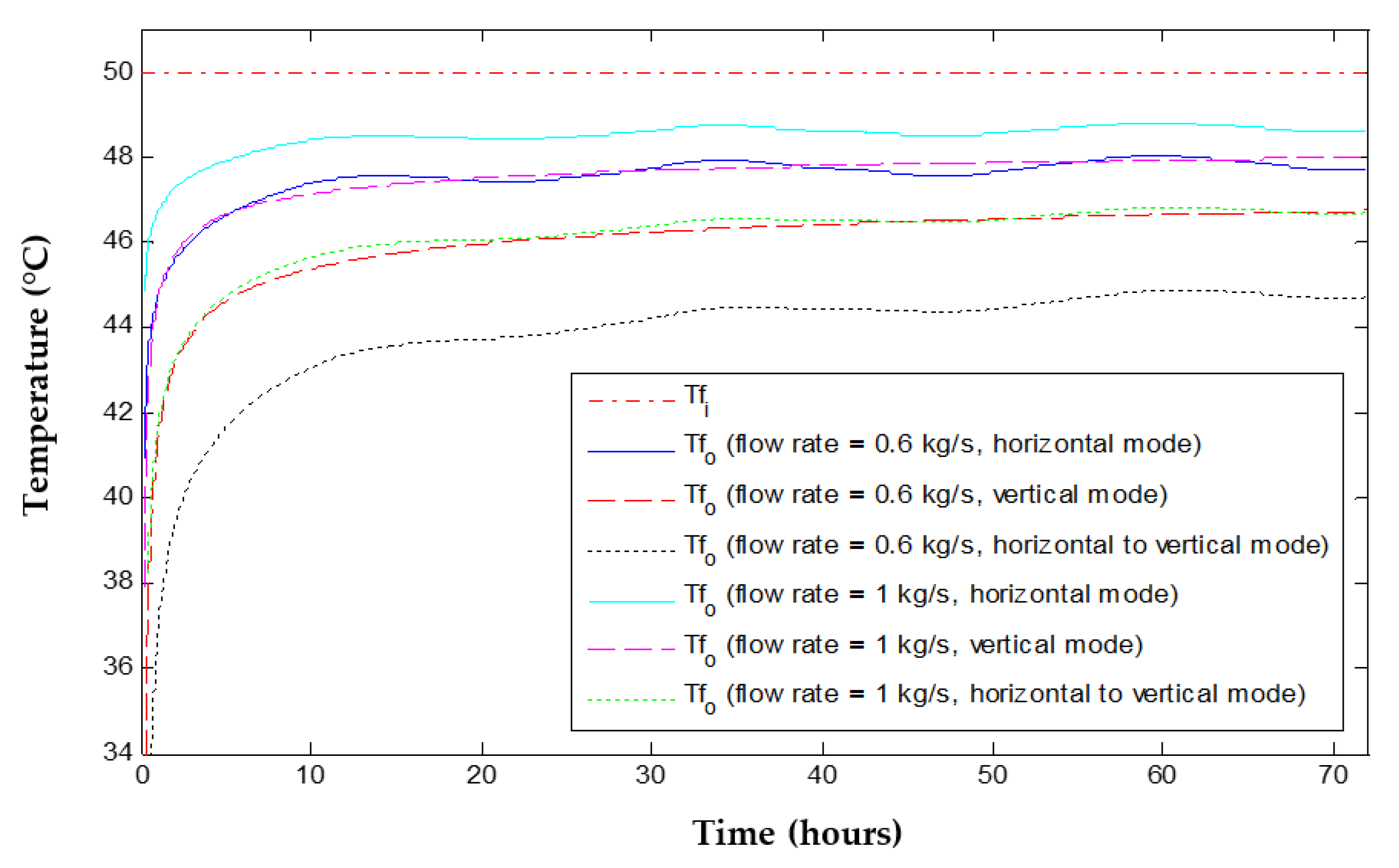
4.5. Variations of the Fluid Mass Flow Rate

Figure 16 shows the effect of the fluid mass flow rate on the amount of energy released by the GHE in 3 summer days in Adelaide. The performance of the GHE under two different fluid mass flow rates namely, 0.6 kg/s and 1 kg/s, was compared. The results of the simulation indicate that the amount of energy released by the GHE increased as the fluid flow rate increased. This tendency occurred because the mass flow rate affected the convective heat transfer coefficient of the fluid inside the GHE. The higher the mass flow rate, the higher the coefficient convective heat transfer was attained. As a result, it increased the heat transfer capacity and the amount of energy released by the GHE. As an example, Figure 17 shows the profile of the fluid temperature generated from the horizontal, vertical, and horizontal to vertical modes at two different mass flow rates namely, 0.6 kg/s and 1 kg/s. This figure shows that the outlet fluid temperature increased with the increase of fluid mass flow rate. This tendency occurred because at a higher mass flow rate, the time period during which the fluid makes contact with the pipe was shorter when compared to a relatively low flow rate. In addition, at a higher mass flow rate, the GHE released more heat into the surrounding soil and led to a quick increase in soil temperature, resulting in increased outlet fluid temperature. Varying the mass flow rate from 0.6 to 1 kg/s increased the amount of energy released by 2.4% for the horizontal mode and 3.3% for the vertical mode. The rate increases were 4.9%, 5.1%, and 5.6% for the horizontal to vertical, vertical to horizontal, and split flow mode, respectively.

5. Conclusions

In this paper, a combined GHE was proposed and its performance in five operational modes was analysed by using the validated models previously developed for horizontal and vertical arrangements of GHEs. The main conclusions, which followed from the calculations, are summarised as follows:
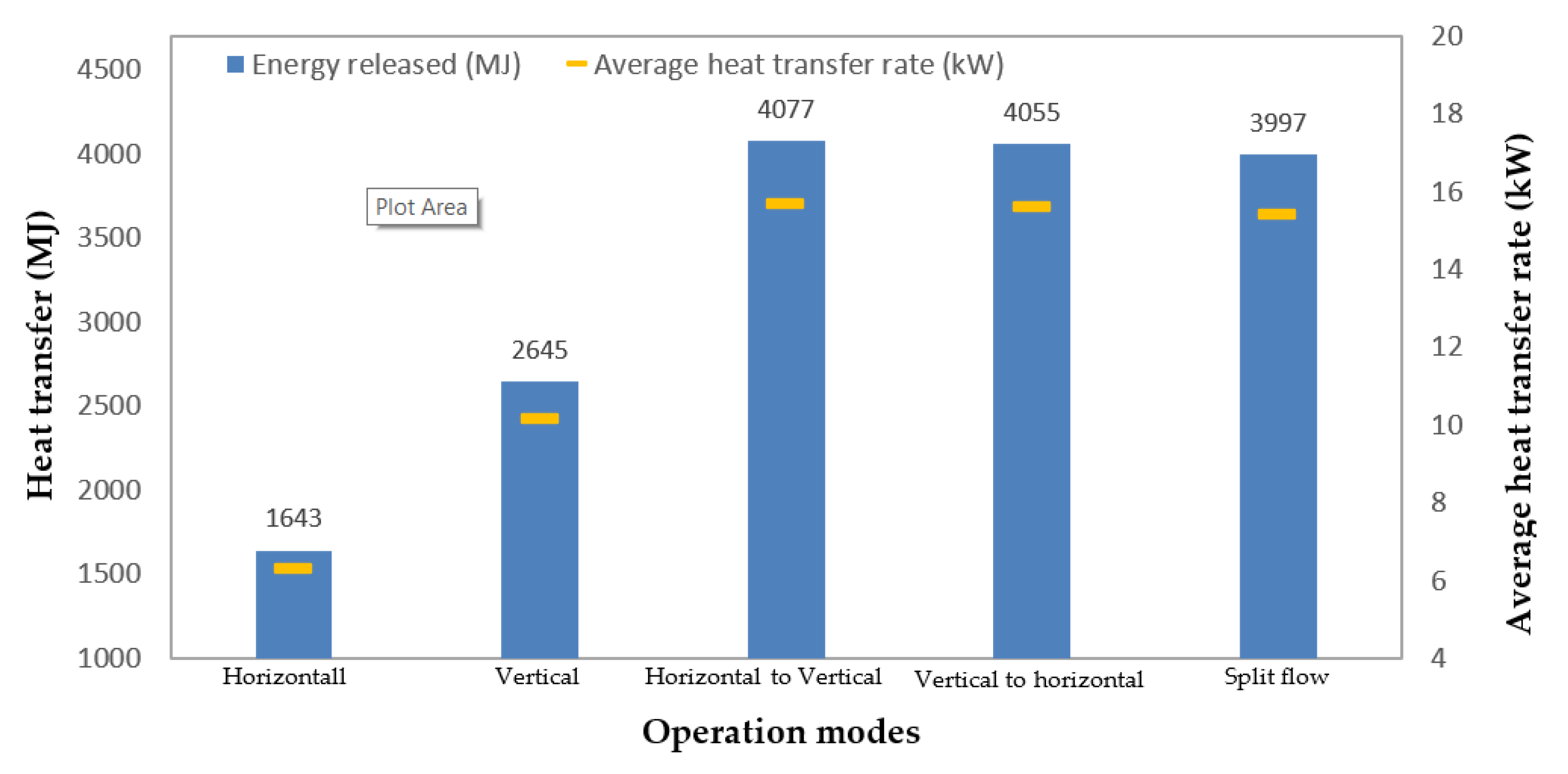
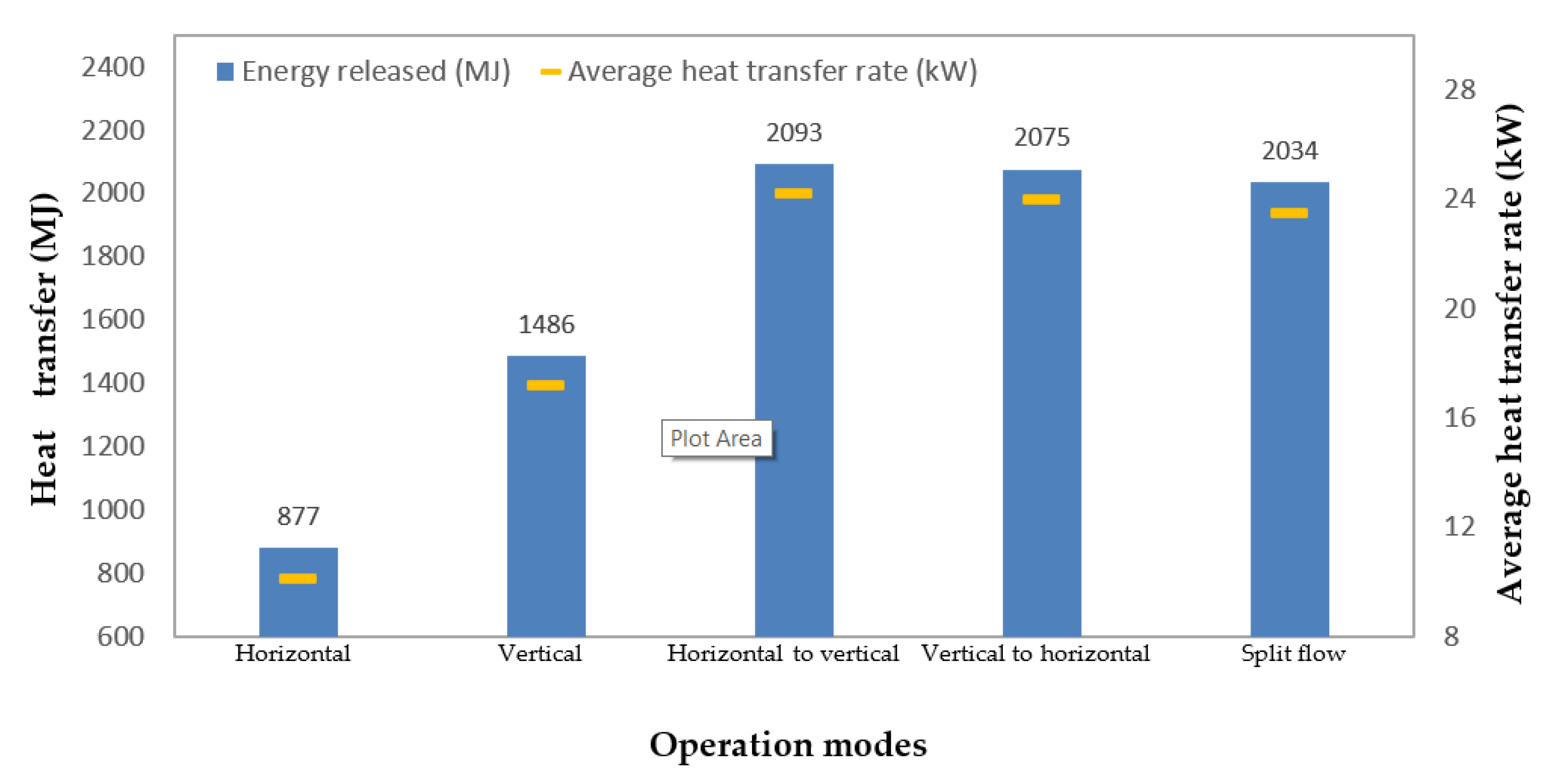
  • With the same length of the pipe system, the vertical GHE could release more energy than the horizontal GHE, as the initial soil temperature (in summer) at a deeper layer was lower than that at a shallow region;
  • When the GHE operated in combined modes, the amount of energy released by the GHE was increased, as the contact area, where heat was exchanged with the surrounding soil, was increased;
  • The series operations (horizontal to vertical or vertical to horizontal) of the GHE could release more energy than could be done in the split mode. The difference in the fluid velocity in the split flow and series modes contributed to the amount of energy released by the GHE;
  • The intermittent operation of the GHE might be conducted to cope with cyclic thermal loading. The intermittent operation could benefit the performance of the GHE as the degradation of the ground temperature during the operation of the GHE was largely recovered during the system shut down.
  • In the split flow mode, the ratio of the fluid mass flow rate did not significantly affect the amount of energy released by the GHE. The GHE with a ratio of mass flow rate of 40% horizontal and 60% vertical releases the highest amount of energy in the split flow operational mode.
  • Climate conditions had a significant effect on the GHE’s performance. The GHE installed in a temperate climate, corresponding to Adelaide’s conditions, could release more energy than the same installation located in a subtropical climate, such as Brisbane. This was due to the difference in the initial soil temperature.
  • Increasing the fluid mass flow rate could enhance the amount of energy released by the GHE as the fluid mass flow rate affected the coefficient of the convective heat transfer of the working fluid.

Author Contributions

Conceptualization, methodology, and results and were initiated and wrote by S.E.S., E.H. and A.K.; S.E.S. contributed to the experiment and writing—original draft preparation; Writing—review and editing, T.M.I.R., R.T.; Supervision by E.H. and A.K. All authors have read and agreed to the published version of the manuscript.

Funding

This research received no external funding.

Acknowledgments

The authors graciously acknowledge the support provided by the School of Mechanical Engineering, the University of Adelaide.

Conflicts of Interest

The authors declare no conflict of interest.

Nomenclature

A area of the pipe (m2) T g grout temperature (K)
A s amplitude of the annual air temperature (K) T m average annual air temperature (°C)
c f fluid specific heat (J/kg K) T p pipe temperature (K)
c s soil specific heat (J/kg K) T ( x , t ) ground temperature at a given depth x on calendar day t (°C)
c p pipe specific heat (J/kg K) T f i inlet fluid temperature (K)
d i n internal pipe diameter (m) T f o outlet fluid temperature
D e q equivalent diameter of the pipe (m) T f m i x final temperature of the mixed fluids (K)
h f convective heat transfer coefficient of fluid (W/(m2 K)) T s soil temperature (K)
H s soil heat source (W/m3) T f o h outlet temperature of the horizontal GHE (K)
k s soil thermal conductivity (W/(m K)) T f o v outlet temperature of the vertical GHE (K)
k g grout thermal conductivity (W/(m K)) v f velocity of the working fluid (m/s)
k v vegetation coefficient ( k v = 1 for bare ground, k v = 0.22 for year round full vegetation cover) V p volume of the pipe’s wall (m3)
L s centre to centre distance between two legs of the U pipe x soil depth (cm)
m ˙ fluid mass flow rate (kg/s) z axial distance of grout domain (m)
m ˙ f fluid mass flow rate (kg/s) α s soil diffusivity (m2/s)
m ˙ f h fluid mass flow rate in the horizontal GHE (kg/s) α g grout diffusivity (m2/s)
m ˙ f v fluid mass flow rate in the vertical GHE (kg/s) ρ f fluid density (kg/m3)
Qenergy released by the GHE (J) ρ p pipe density (kg/m3)
Q ˙ c a Convective heat transfer on the ground surface (W) ρ s soil density (kg/m3)
Q ˙ c f Convective heat transfer on the inner pipe surface (W) Δ t time period (s)
r radius of soil domain (m) Δ T m local site variable for the ground temperature (K)
r b radius of the borehole ρ f fluid density (kg/m3)
t time period (s) Δ T s soil temperature difference in summer and winter (K)
t 0 phase of air temperature wave (day) Δ r radial increment (m)
t c calendar day, where 1 January = 1 and so forth Δ z distance in the direction parallel to the pipe (m)
T f fluid temperature (K) ψ Courant number

References

  1. Sliwa, T.; Gonet, A. Theoretical Model of Borehole Heat Exchanger. J. Energy Resour. Technol. 2004, 127, 142–148. [Google Scholar] [CrossRef]
  2. Florides, G.; Christodoulides, P.; Pouloupatis, P. Single and double U-tube ground heat exchangers in multiple-layer substrates. Appl. Energy 2013, 102, 364–373. [Google Scholar] [CrossRef]
  3. Zhai, X.; Qu, M.; Yu, X.; Yang, Y.; Wang, R. A review for the applications and integrated approaches of ground-coupled heat pump systems. Renew. Sustain. Energy Rev. 2011, 15, 3133–3140. [Google Scholar] [CrossRef]
  4. Dai, L.; Li, S.; Duanmu, L.; Li, X.; Shang, Y.; Dong, M. Experimental performance analysis of a solar assisted ground source heat pump system under different heating operation modes. Appl. Therm. Eng. 2015, 75, 325–333. [Google Scholar] [CrossRef]
  5. Kjellsson, E.; Hellström, G.; Perers, B. Optimization of systems with the combination of ground-source heat pump and solar collectors in dwellings. Energy 2010, 35, 2667–2673. [Google Scholar] [CrossRef]
  6. Ozgener, O.; Hepbasli, A. Experimental performance analysis of a solar assisted ground-source heat pump greenhouse heating system. Energy Build. 2005, 37, 101–110. [Google Scholar] [CrossRef]
  7. Yang, W.; Sun, L.; Chen, Y. Experimental investigations of the performance of a solar-ground source heat pump system operated in heating modes. Energy Build. 2015, 89, 97–111. [Google Scholar] [CrossRef]
  8. Zajacs, A.; Lalovs, A.; Borodinecs, A.; Bogdanovics, R. Small ammonia heat pumps for space and hot tap water heating. Energy Procedia 2017, 122, 74–79. [Google Scholar] [CrossRef]
  9. Park, H.; Lee, J.S.; Kim, W.; Kim, Y. Performance optimization of a hybrid ground source heat pump with the parallel configuration of a ground heat exchanger and a supplemental heat rejecter in the cooling mode. Int. J. Refrig. 2012, 35, 1537–1546. [Google Scholar] [CrossRef]
  10. Man, Y.; Yang, H.; Wang, J. Study on hybrid ground-coupled heat pump system for air-conditioning in hot-weather areas like Hong Kong. Appl. Energy 2010, 87, 2826–2833. [Google Scholar] [CrossRef]
  11. Wang, S.; Liu, X.; Gates, S. Comparative study of control strategies for hybrid GSHP system in the cooling dominated climate. Energy Build. 2015, 89, 222–230. [Google Scholar] [CrossRef] [Green Version]
  12. Sagia, Z.; Rakopoulos, C.D.; Kakaras, E. Cooling dominated Hybrid Ground Source Heat Pump System application. Appl. Energy 2012, 94, 41–47. [Google Scholar] [CrossRef]
  13. Fan, R.; Gao, Y.; Hua, L.; Deng, X.; Shi, J. Thermal performance and operation strategy optimization for a practical hybrid ground-source heat-pump system. Energy Build. 2014, 78, 238–247. [Google Scholar] [CrossRef]
  14. Canelli, M.; Entchev, E.; Sasso, M.; Yang, L.; Ghorab, M. Dynamic simulations of hybrid energy systems in load sharing application. Appl. Therm. Eng. 2015, 78, 315–325. [Google Scholar] [CrossRef]
  15. Zhu, N.; Hu, P.; Lei, Y.; Jiang, Z.; Lei, F. Numerical study on ground source heat pump integrated with phase change material cooling storage system in office building. Appl. Therm. Eng. 2015, 87, 615–623. [Google Scholar] [CrossRef]
  16. Wu, W.; Li, X.; You, T.; Wang, B.; Shi, W. Combining ground source absorption heat pump with ground source electrical heat pump for thermal balance, higher efficiency and better economy in cold regions. Renew. Energy 2015, 84, 74–88. [Google Scholar] [CrossRef]
  17. You, T.; Shi, W.; Wang, B.; Wu, W.; Li, X. A new ground-coupled heat pump system integrated with a multi-mode air-source heat compensator to eliminate thermal imbalance in cold regions. Energy Build. 2015, 107, 103–112. [Google Scholar] [CrossRef]
  18. Li, X.; Lyu, W.; Ran, S.; Wang, B.; Wu, W.; Yang, Z.; Jiang, S.; Cui, M.; Song, P.; You, T.; et al. Combination principle of hybrid sources and three typical types of hybrid source heat pumps for year-round efficient operation. Energy 2020, 193, 116772. [Google Scholar] [CrossRef]
  19. Hou, G.; Taherian, H.; Li, L.; Fuse, J.; Moradi, L. System performance analysis of a hybrid ground source heat pump with optimal control strategies based on numerical simulations. Geothermics 2020, 86, 101849. [Google Scholar] [CrossRef]
  20. Allaerts, K.; Coomans, M.; Salenbien, R. Hybrid ground-source heat pump system with active air source regeneration. Energy Convers. Manag. 2015, 90, 230–237. [Google Scholar] [CrossRef]
  21. Sofyan, S.E.; Hu, E.; Kotousov, A.; Kotousov, A. A new approach to modelling of a horizontal geo-heat exchanger with an internal source term. Appl. Energy 2016, 164, 963–971. [Google Scholar] [CrossRef]
  22. Sofyan, S.E.; Hu, E.; Kotousov, A.; Riayatsyah, T.M.I.; Khairil; Hamdani. A new approach to modelling of seasonal soil temperature fluctuations and their impact on the performance of a shallow borehole heat exchanger. Case Stud. Therm. Eng. 2020, 22, 100781. [Google Scholar] [CrossRef]
  23. Sofyan, S.E.; Hu, E.; Kotousov, A. Modelling of a Horizontal Geo Heat Exchanger with an Internal Source Term Approach. Energy Procedia 2014, 61, 104–108. [Google Scholar] [CrossRef] [Green Version]
  24. Baggs, S.A. Remote prediction of ground temperature in Australian soils and mapping its distribution. Sol. Energy 1983, 30, 351–366. [Google Scholar] [CrossRef]
  25. Gu, Y.; O’Neal, D.L. Development of an equivalent diameter expression for vertical U-tube used in ground-coupled heat pumps. ASHRAE Trans. 1998, 104, 347–355. [Google Scholar]
  26. Zima, W.; Dziewa, P. Modelling of liquid flat-plate solar collector operation in transient states. Proc. Inst. Mech. Eng. Part A J. Power Energy 2011, 225, 53–62. [Google Scholar] [CrossRef]
  27. Geoserver, S.A.R.I. Soil Association Map. Available online: https://sarigbasis.pir.sa.gov.au/WebtopEw/ws/plans/sarig1/image/DDD/200471-235 (accessed on 4 October 2020).
  28. Prangnell, J.; McGowan, G. Soil temperature calculation for burial site analysis. Forensic Sci. Int. 2009, 191, 104–109. [Google Scholar] [CrossRef]
  29. Australian Government Bureau of Meteorology. Climate Data Online. Available online: http://www.bom.gov.au/climate/data/?ref=ftr (accessed on 4 October 2020).
Figure 1. (a) Schematic of the horizontal geothermal heat exchanger (GHE). (b) Schematic of the vertical GHE.
Energies 13 06598 g001
Figure 2. Schematic of the hybrid horizontal vertical GHE.
Energies 13 06598 g002
Figure 3. Schematic of the vertical GHE with an equivalent diameter.
Energies 13 06598 g003
Figure 4. Computational domain of the vertical GHE.
Energies 13 06598 g004
Figure 5. Typical soil temperature in Adelaide and Brisbane.
Energies 13 06598 g005
Figure 6. An example of ambient temperature in Adelaide and Brisbane on 3 consecutive summer days.
Energies 13 06598 g006
Figure 7. The absolute value of the internal heat source at various depths.
Energies 13 06598 g007
Figure 8. Energy released in 3 days and average heat transfer rate of the GHE under continuous operation condition in Adelaide (where the inlet fluid temperature = 50 °C, fluid mass flow rate = 0.6 kg/s, length of horizontal GHE = 200 m, length of vertical GHE = 200 m).
Energies 13 06598 g008
Figure 9. Profile of fluid temperature of the horizontal, vertical, and horizontal to the vertical mode in Adelaide.
Energies 13 06598 g009
Figure 10. Energy released in 3 days and average heat transfer rate of the GHE under intermittent operation in Adelaide (where the inlet fluid temperature = 50 °C, fluid mass flow rate = 0.6 kg/s, length of horizontal GHE = 200 m, and length of vertical GHE = 200 m).
Energies 13 06598 g010
Figure 11. Profile of the fluid temperature of the horizontal to the vertical mode in Adelaide.
Energies 13 06598 g011
Figure 12. Energy released in 3 days by the GHE with different ratio of mass flow rate in Adelaide (where the inlet fluid temperature = 50 °C, fluid mass flow rate = 0.6 kg/s, length of horizontal GHE = 200 m, and length of vertical GHE = 200 m).
Energies 13 06598 g012
Figure 13. Profile of the outlet fluid temperature of the GHE (with a split flow operation mode) under different flow rate ratios (Adelaide case).
Energies 13 06598 g013
Figure 14. Energy released in 3 days by the GHE under different climate conditions (where the inlet fluid temperature = 50 °C, fluid mass flow rate = 0.6 kg/s, length of horizontal GHE = 200 m, and length of vertical GHE = 200 m).
Energies 13 06598 g014
Figure 15. Profile of fluid temperatures of the horizontal, vertical, and the horizontal to vertical modes under different climate conditions.
Energies 13 06598 g015
Figure 16. Energy released in 3 days by the GHE with different mass flow rate in Adelaide (where the inlet fluid temperature = 50 °C, length of horizontal GHE = 200 m, and length of vertical GHE = 200 m).
Energies 13 06598 g016
Figure 17. Profile of fluid temperature of the horizontal, vertical, and the horizontal to vertical modes with variations in the fluid mass flow rates, in Adelaide.
Energies 13 06598 g017
Table 1. The parameters of the reference case.
ParametersValueUnitParametersValueUnit
Horizontal GHE--Circulation fluid (water)--
Total pipe length (L)200mInlet water temperature ( T f i )50°C
Burial depth (h)0.25mFlow rate ( m ˙ f )0.6kg/s
Pipe internal diameter ( d i n )0.04mSpecific heat ( c f )4188J/kg K
Pipe outer diameter ( d o u t )0.044mDensity ( ρ f )980kg/m3
Centre distance between pipe ( L s )0.28mSoil type in Adelaide: layered old dune sands [27]--
Distance of soil domain in x direction (z)0.14mThermal conductivity ( k s )1.3W/m K
Distance of soil domain in y direction (z)1.5mSpecific heat ( c s )1140J/kg K
Vertical GHE--Density ( ρ s )1500kg/m3
Total pipe length (L)200mSoil type in Brisbane: clay [28]--
Borehole depth (h)100mThermal conductivity ( k s )1.1W/m K
Borehole diameter ( D b )0.15mSpecific heat ( c s )1500J/kg K
Soil domain diameter ( D s )4mDensity ( ρ s )1300kg/m3
Pipe internal diameter ( d i n )0.04mGrout (vertical GHE)
Pipe outer diameter ( d o u t )0.044mThermal conductivity ( k g )2W/m K
Centre distance between pipes ( L s )0.07mSpecific heat ( c g )1140J/kg K
Density ( ρ g )1500kg/m3
Wind speed (Adelaide)4.9m/s
Wind speed (Brisbane)3.8m/s
Table 2. The parameters reference used to estimate the soil temperature.
ParameterAdelaideUnitBrisbaneUnit
Average annual air temperature (Tm)16.45°C25.4°C
Amplitude of the annual air temperature (As)11.9°C11.2°C
The local site variable for the ground temperature (∆Tm)2.5°C3°C
Vegetation coefficient ( k v )1-1-
Soil thermal diffusivity (α)0.7610−2 cm−2 s−10.5510−2 cm−2 s−1
Phase of air temperature wave (t0)10 (10 January)day19 (19 January)Day
Publisher’s Note: MDPI stays neutral with regard to jurisdictional claims in published maps and institutional affiliations.

