Article

Design and Implementation of Model Predictive Control Based PID Controller for Industrial Applications

1
Electrical and Control Engineering Department, College of Engineering & Technology, Arab Academy for Science, Technology and Maritime Transport (AASTMT), Alexandria 1029, Egypt
2
Key Laboratory of More Electric Aircraft Technology of Zhejiang Province, University of Nottingham, Ningbo 315100, China
*
Author to whom correspondence should be addressed.
Energies 2020, 13(24), 6594; https://doi.org/10.3390/en13246594
Submission received: 7 October 2020 / Revised: 27 November 2020 / Accepted: 30 November 2020 / Published: 14 December 2020
(This article belongs to the Section A1: Smart Grids and Microgrids)

Abstract

:
Advanced control approaches are essential for industrial processes to enhance system performance and increase the production rate. Model Predictive Control (MPC) is considered as one of the promising advanced control algorithms. It is suitable for several industrial applications for its ability to handle system constraints. However, it is not widely implemented in the industrial field as most field engineers are not familiar with the advanced techniques conceptual structure, the relation between the parameter settings and control system actions. Conversely, the Proportional Integral Derivative (PID) controller is a common industrial controller known for its simplicity and robustness. Adapting the parameters of the PID considering system constraints is a challenging task. Both controllers, MPC and PID, merged in a hierarchical structure in this work to improve the industrial processes performance considering the operational constraints. The proposed control system is simulated and implemented on a three-tank benchmark system as a Multi-Input Multi-Output (MIMO) system. Since the main industrial goal of the proposed configuration is to be easily implemented using the available automation technology, PID controller is implemented in a PLC (Programable Logic Controller) controller as a lower controller level, while MPC controller and the adaptation mechanism are implemented within a SCADA (Supervisory Control And Data Acquisition) system as a higher controller level.

1. Introduction

Industrial processes have become more complex and contain several control loops. The Proportional Integral Derivative (PID) controller is considered the most popular control loop for field engineers and plant operators due to its simple structure. Approximately 1/3 of control loops in plants utilize traditional PID controllers, while the other loops need to be enhanced through advanced control techniques [1]. In a typical plant, control loops are complex and require advanced control algorithms for lower costs and better performance. As a result, the tuning of the PID controller becomes challenging for field engineers especially for a process with multiple interacting loops, time delays, constraints, nonlinearities and uncertainties [2].
Several PID controller-tuning methods have been presented in the literature [3,4,5]. Many are based on the analysis of system responses to test signals and empirical rules, for instance, the Zigler-Nicholes and Cohen-Coon methods [6,7]. Some of the tuning methods use the modified PID controller such as Fractional Order PID [8,9] and Internal Model Control [10,11]. Artificial intelligence techniques could be used to adapt PID gains such as Fuzzy PID [12,13], Genetic Algorithm [14,15] and Neural Network [16]. Additionally, other advanced PID tuning techniques are available based on multi-objective optimization [17] or predictive control [18,19]. The adaptation techniques of the PID controller based on the advanced control theory, stated before, achieve the required target. However, most techniques remain in the research phase and have not been applied in industries mainly due to human and technology constraints. Moreover, most of these techniques are designed for a single control loop. Hence, it is necessary to design an adaptation technique that can be practically implemented in the industry for multiple PID loops for Multi-Input Multi-Output (MIMO) system.
Industrial plants can increase the profit and product quality and decrease the overall costs through the implementation of appropriate process control and optimization tools, which is known as Advanced Process Control (APC) and can be implemented by advanced automation system technology such as Distributed Control System (DCS). The APC covers different control techniques such as feed-forward control, cascade control, time delay compensators, supervision, multivariable, nonlinear and Model Predictive Control (MPC), adaptive algorithms and so forth [20]. To deal with the APC, three major factors should be considered as shown in Figure 1.
In the industrial field, the majority of operators are familiar with traditional control techniques rather than advanced control approaches, these approaches require more qualifications and expertise. Nevertheless, the APC algorithms require advanced automation technology and devices in contrast to traditional control techniques. Thus, the main challenge of APC remains to be the controller design through a combination of the existing automation technology and field operators’ knowledge as illustrated in Figure 1. The application of advanced control theory should be in a simple manner to facilitate the understanding and executability of the APC by field engineers and plant operators.
Since the industrial automation system is constructed in a multi-leveled or hierarchal structure [21,22], the advanced control algorithm can be applied centrally or distributed among different levels of automation hierarchy of the industrial plant to meet the APC challenges. Consequently, most advanced control theory is performed in a hierarchical control structure in various applications, for example, power system [23] and robotics [24]. MPC is an APC algorithm that has significant advantages, particularly for the MIMO system with constraints [25,26,27,28]. Regardless of the MPC effectiveness, it is still applied at the supervisory level for most industrial applications in optimizing the set point of the process instead of regulating the control loop due to human constraints and computational burden [29,30,31]. As stated above, PID remains preferred for industrial control loops as it is elementary and comprehensible by field engineers. The classical tuning of PID control is deemed ineffective in controlling industrial plants. This suggests that adopting the PID controller based on the APC technique is necessary. For this purpose, a combination of PID and MPC is recommended to be implemented in industrial applications. The PID controller adaptation based on MPC was introduced in References [32,33] for a Single-Input Single-Output (SISO) system without constraints. In this paper, the proposed technique adapts PID gains for MIMO with constraints based on MPC. This technique is applied in two stages: (1) Designing an MPC controller that achieves the required performance for a constrained MIMO system; (2) Identifying PID gains that give a similar performance of MPC by employing the Recursive Least Square (RLS) identification method.
The control task is implemented in a hierarchal control configuration of two levels as shown in Figure 2. Since the PID controller must satisfy a rapid response time for the controlled process, it will be implemented in the lower level, such as Programable Logic Controller (PLC) or other individual controllers. In contrast, the adaptation mechanism rate is slower than the sampling one of the process. Hence, the MPC control loop and the adaptation algorithm will be executed at the upper controller level such as SCADA system. This configuration allows the proposed technique to be suitable for different industrial processes.
To validate the proposed technique, an experimental nonlinear MIMO three-tank system is used to implement the proposed technique as it is a common benchmark that simulates many industrial processes, for example, wastewater treatment stations, petroleum refining plants and so forth. Other uses include testing and validating different control techniques and strategies [34].
Therefore, the main contributions of this paper are summarized as (1) Design an adaptation technique of PID for MIMO considering process constraints, human and existing technology constraints as well; (2) Integrate MPC, as one of the effective APC techniques, with PID to adapt its loop instead of adjusting the setpoint only; (3) Implement the control algorithm in a hierarchical structure considering the human background and industrial technology constraints, functionality and computational burden; (4) Validate the proposed technique on an experimental benchmark using industrial automation technology.
The remaining of this paper is organized as follows. Section 2 shows the proposed algorithm. Section 3 illustrates the simulation results of the proposed technique for the three-tank system. The experimental system and results are described in Section 4 and the conclusion is discussed in Section 5.

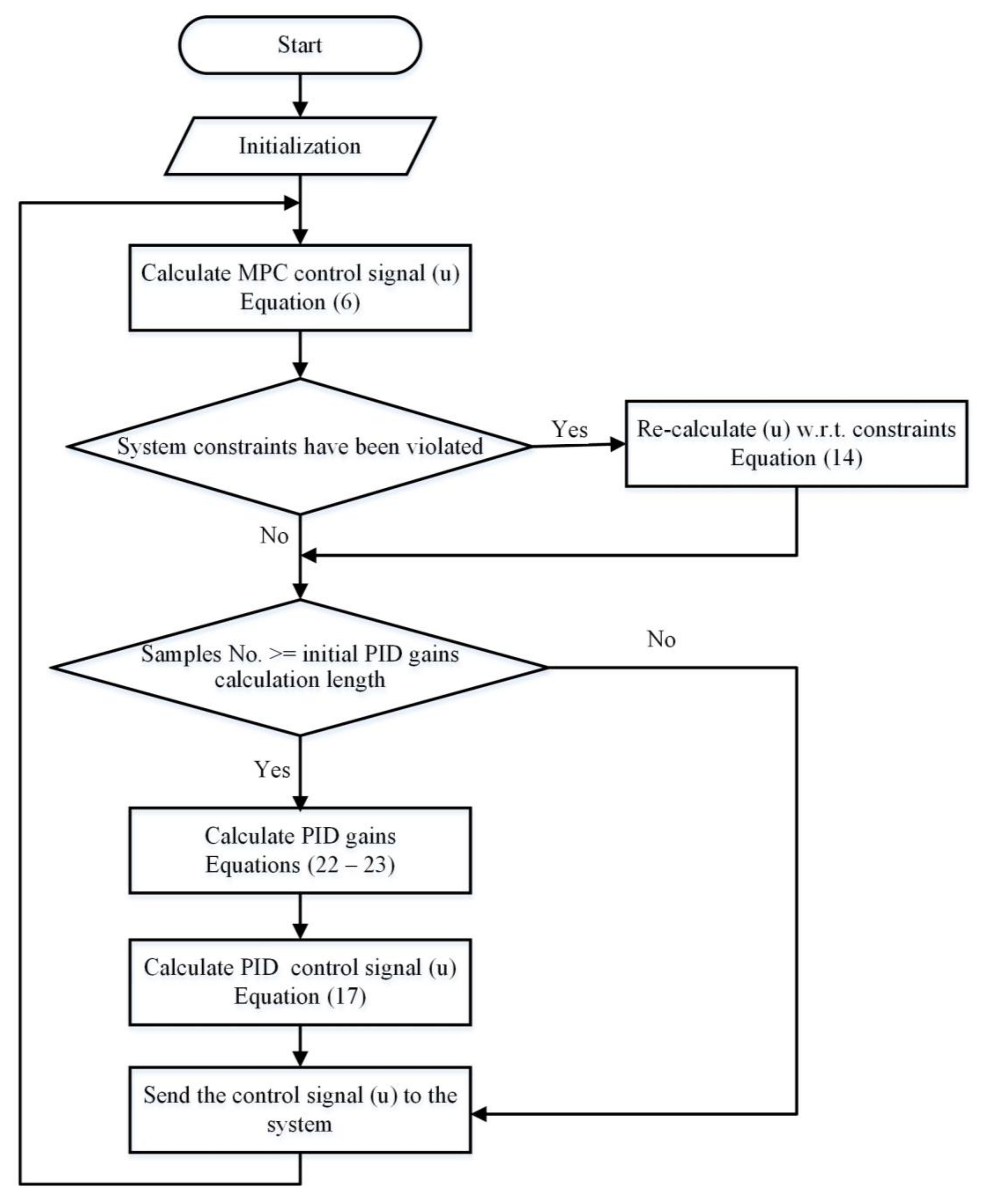
2. The Proposed Algorithm

The focus of the proposed method is to develop an online tuning mechanism of PID controllers for MIMO systems with constraints that can be implemented using industrial automation technology considering the human background. The algorithm is sectioned into two parts: Firstly, the control vector is computed using MPC; Secondly, PID controllers’ parameters are computed using the MPC output based on the RLS identification method.

2.1. MPC Design

MPC is applied for several industrial applications, which require higher performance and more robustness. The control signal is obtained by minimizing the cost function given by References [35,36]:
j = k = 1 n y e T k Q k e k + k = 0 n u 1 u T k R k u k ,
subject to a discrete state-space model:
x k + 1 = A x k + B u k
y k = C x k + D u k ,
where e k l 1 = y k l 1 r k l 1 is the error, y k l 1 is the system output, r k l 1 is the system reference, u k m 1 is the system input, Q k l l and R k m m are weighting matrices, x k n 1 is the system states, A n n ,   B n m   ,   C l n ,   D l m are the system parameters, ny is the prediction horizon value, nu is the control horizon value, m is the number of inputs, l is the number of outputs and n is the number of states. The recursive form of the model over the prediction horizon ny is given by:
x ^ k + 1 = P x   x k + H x   u ^ k
y ^ k + 1 = P   x k + H   u ^ k ,
where:
x ^ k + 1 = x k + 1 x k + 2 x k + 3 x k + n y ,   u ^ k = u k u k + 1 u k + 2 u k + n y 1 ,   P x = A A 2 A 3 A n y ,   H x = B 0 0 AB B 0 A 2 B AB B A n y 1 B A n y 2 B A n y 3 B ,
y ^ k + 1 = y k + 1 y k + 2 y k + 3 y k + n y ,   P = CA CA 2 CA 3 CA n y ,   H = CB 0 0 CAB CB 0 CA 2 B CAB CB CA n y 1 B CA n y 2 B CA n y 3 B .
x ^ k + 1 n n y 1 is the predicted system states, u ^ k m n y 1   is the system input, y ^ k + 1 l n y 1 is the system output, and P x n n y n , H x n n y m n y ,   P l n y n , H l n y m n y are the system parameters over the prediction horizon ny. The minimization of (1) with respect to u k without considering the variable constraints is given by:
u k MPC = L [ ( H T Q ^ k H + H T Q ^ T k H + 2 R ^   T k ) 1   2 H T Q ^ T k r ^ k P x k ] ,
where L m m n y = I m m   : O m m n y m , Im*m is an identity matrix and Om*(m*ny-m) is a zero matrix, r ^ k l n y 1 is the system reference, Q ^ k l n y l n y and R ^ k m n u 1 m n u 1 are weighting matrices. Solving the constrained optimization problem is considered one of MPC’s main aspects. System constraints can be represented in the inputs, inputs rates, outputs and states such as:
u _ k u k u ¯ k
Δ u _ k Δ u k Δ u ¯ k
y _ k y k y ¯ k
x _ k x k x ¯ k .
Since the output y k and x k are functions of the control input u k , then the state and output constraints can be presented generally as additional constraints for the input in the form of:
W k u k f k ,
where W k n c m and f k n c 1 are representing the system constraints parameters according to constraints number nc. The softening constraints method is one of the constraint handling methods and it requires a lower computational burden than other approaches [37,38]. In this method, the violation between the input signal and their constraints is merged into the cost function such as:
j = k = 1 n y e T k Q k e k + k = 0 n u 1 u T k R k u k + k = 0 n u 1 W k u k f k T S k W k u k f k ,
where S k m m is the weighting matrix. Considering the maximum input constraint:
u k   u ¯ k m 1  
then
f   =   u ¯ k     and   W ( k )   =   I ,
where u ¯ k m 1   is the upper boundary of the control signal. The control signal that minimizes the function (12) is given by:
u k MPC = L [ H T Q ^ k H + H T Q T k H + 2 R ^   T k + 2 S ^ T k 1 2 H T Q ^ T k r ^ k P x k + 2 S ^ T k u ¯ ^ k ]   ,
where u ¯ ^ k m n u 1 1 and S ^ k m n u 1 m n u 1 are the maximum limits of control signal and weighting matrix over the control horizon n u 1 . The proper selection of the weighting matrices Q k and R ( k ) is essential for the controller design to penalize the states or control inputs. Larger weighting values means more restricted variables. A design approach can be used to obtain the optimum values for the weighting factors [39]. By obtaining the control signal, u(k)MPC, it is required to adjust the PID controllers’ gains to satisfy the same behavior of MPC.

2.2. PID Controller Tuning
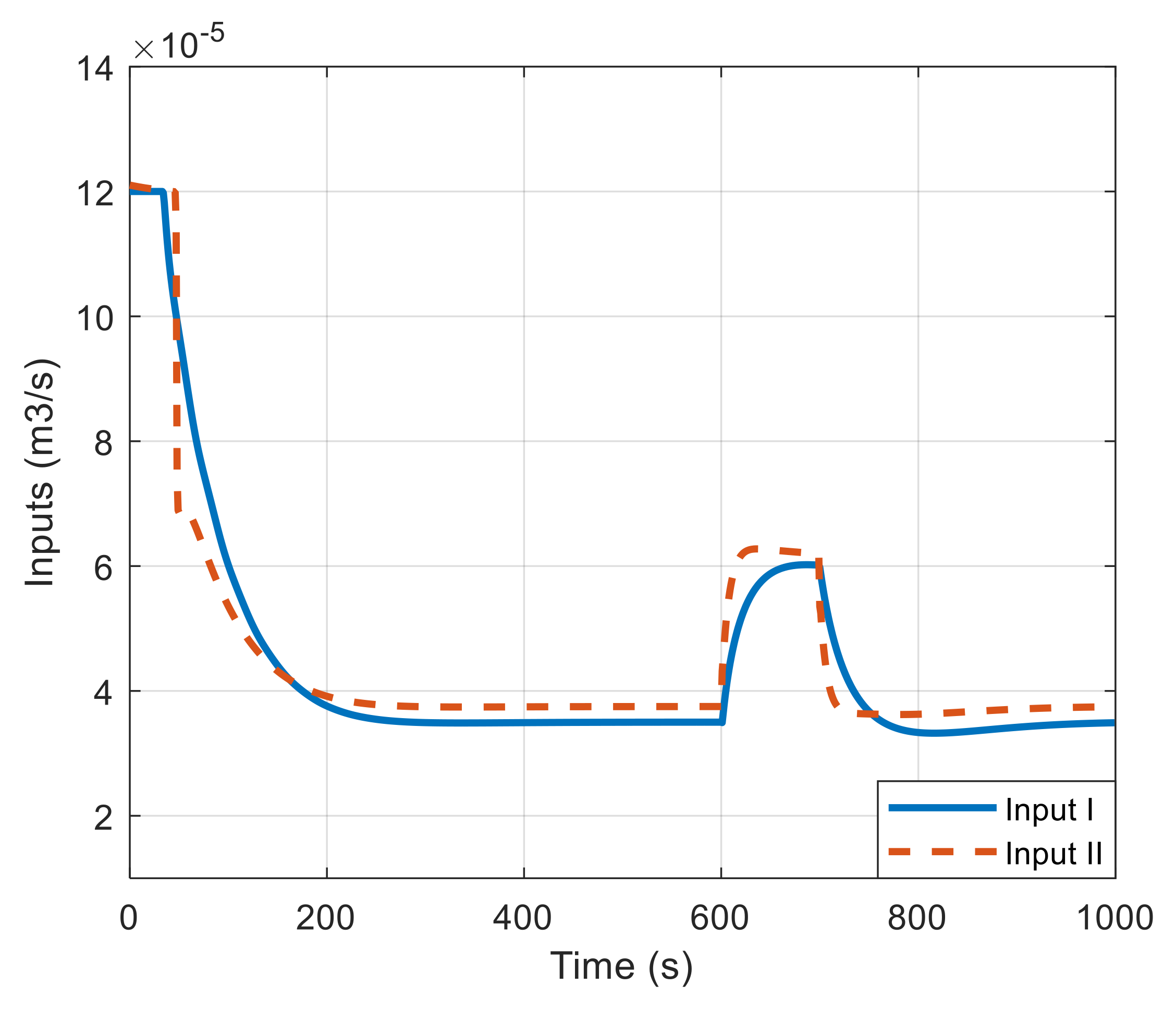
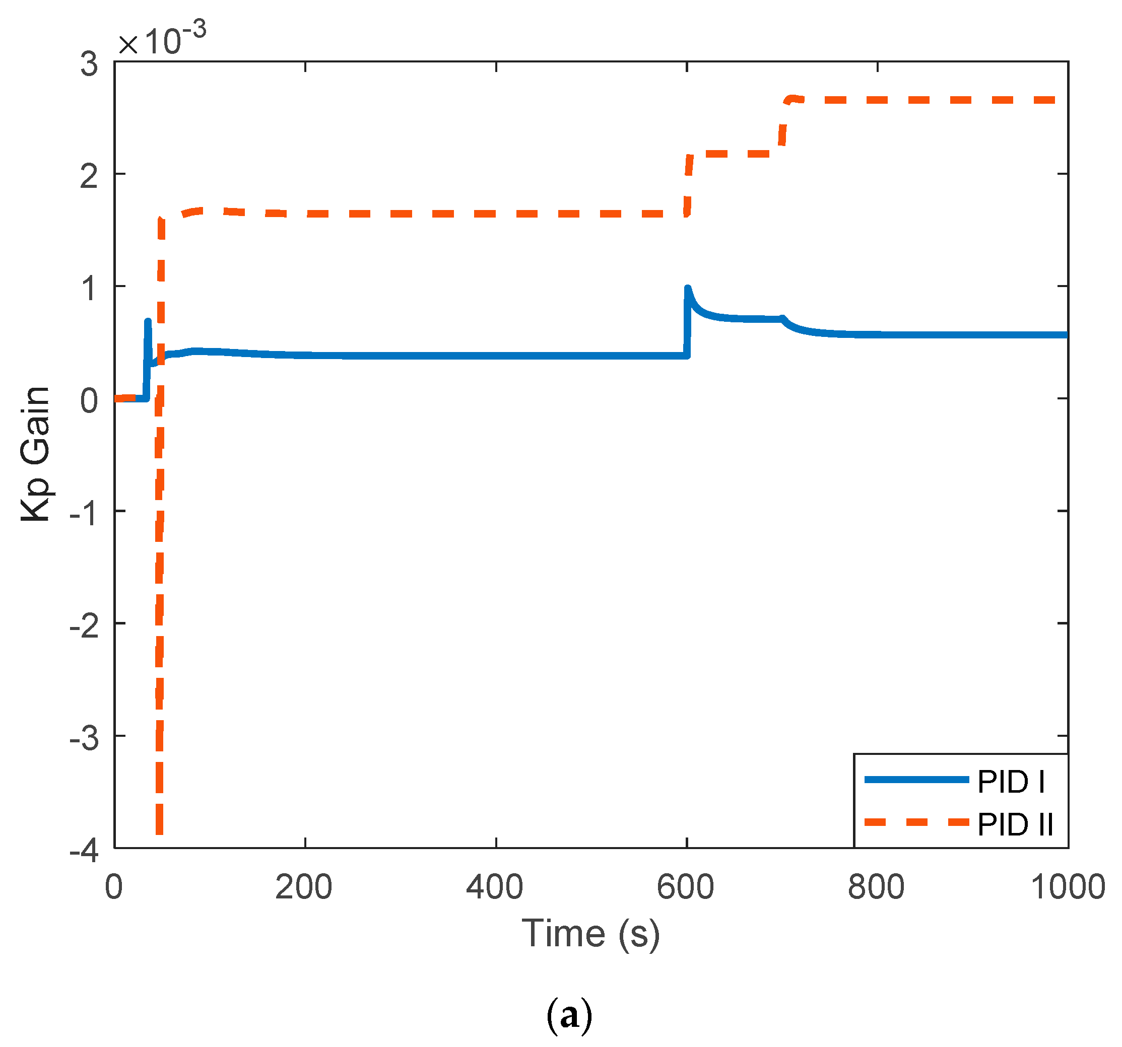
The general representation of the MIMO system is illustrated in Figure 3 employing C l m as a MIMO controller. In the case of PID controller it will be:
C s = c 11 c 1 l c m 1 c m l = ( k P 11 + k I 11 s + k D 11 s ) k P 1 l + k I 1 l s + k D 1 l s ( k P m 1 + k I m 1 s + k D m 1 s ) k P l m + k I l m s + k D m l s ,
where the number of PID controllers is l∗m and the total number of PID gains is the triple of l∗m. The continuous control signal u i t is obtained from:
u i t = j = 1 l k P i j e j t + k I i j e j t d t + k D i j d d t e j t
where e j t is the error, k P i j , k I i j and k D i j are the proportional, integral and derivative controller parameters for controller i ϵ   1 , 2 , m due to error signal j ϵ 1 , 2 , l . The discrete form of (16) can be represented as:
u i k = j = 1 l k P i j Δ e j k + k I i j T s e j k + k D i j T s Δ 2 e j k + u i j k 1 ,
where
Δ e j k = ( e j k e j k 1 ) ,   Δ 2 e j k = ( e j k 2 e j k 1 + e j k 2 )  
e j k , e j k 1 , e j k 2 are the error and Ts is the sampling time, then:
Δ u i k = u i k j = 1 l ( u i j k 1 ) = k P i 1   k I i 1   k D i 1     k P i l   k I i l   k D i l e j t   T s e j k   2 e j k T s     e j t   T s e j k 2 e j k T s T   .
The adaptation of PID gains is achieved using the RLS identification method based on MPC which will be implemented in the supervisory level controller; for example, DCS or SCADA system. As for the realization of PID, it will be executed in the field level controller (i.e., PLC) as illustrated in Figure 4. The RLS is considered an effective technique for estimating the parameters of a linear regression system. The identified PID model can be obtained by Reference [40]:
y k = 𝛉 T   Ψ k + ε k   ,
where θ is a column vector of parameters to be estimated from observations y k and Ψ k , while ε k is the noise. Then, a quadratic cost function based on the sum of the squares of the difference between the observed output and model predictions is obtained as follows:
j 𝛉 = 1 K k = 1 K α k y k 𝛉 T Ψ k 2 ,
where αk is a weighting scalar coefficient. In the case of a linearized system, such as the three-tank system in Section 3, a forgetting technique is used by forgetting the old samples [40] that make the weighting scale coefficient adaptable and it is obtained by:
α k = ρ K k δ k ,
where ρ is the forgetting factor, K is the estimation length, k is the sample number and δ k is the nominal scale factor for sample number k. The updated parameters 𝛉 k are given by:
𝛉 k = 𝛉 k 1 + G 1 k α k Ψ k   y k Ψ T k 𝛉 k 1 .
By applying the identification algorithm on the PID model in (18), considering:
𝛉 k = [ k P i 1   k I i 1   k D i 1     k P i l   k I i l   k D i l ] T
Ψ k = Δ e 1 k t s e 1 k Δ e 1 k t s Δ e l k t s e l k Δ e l k t s T
y k = Δ u i k M P C = u i k M P C u k 1 M P C .
The controller parameters in (23) will be estimated according to (20) and the number of initial samples in the recursive formula should be equal or greater than the number of PID gains to be estimated. To guarantee the proposed controller stability, let Uom is the possible control signal subspace which satisfies (11), where u MPC ∈ Uo= {u| W k u k f k } and Ҡ ⊆ 3m is the subspace of all possible values of PID controller parameters,   𝛉 . , in (23). Since terminal constraints ensure the stability of the MPC controller as discussed in Reference [34], then to ensure the stability of the adapted PID controller based on MPC is:
𝛉     Ҡ = {   𝛉 | u PID U o   } ,
where u PID is the control signal of the PID controller in (17). The control algorithm is computed based on the flow chart in Figure 5.

3. Simulation

The proposed control technique has been tested on the experimental three-tank system shown in Figure 6. For the three-tank system, the control problem is to maintain the levels at predefined values. The system is linearized around the operating point using Taylor expansion by considering the assumption L1>L3>L2. As illustrated in Figure 6, the system consists of three identical cylindrical tanks with equal cross-section area At. These tanks are connected by two pipes of the same cross-section area Ap and have the same outflow coefficient µ13 and µ32. The nominal outflow is located at the second tank and it has the same cross-section area as the coupling pipe between the cylinders but with a different outflow coefficient µ20. Two pumps control the inlet flow to the first and second tanks, whereas the third tank is uncontrollable. So, it is affected by the level in the two end tanks. Pumps flow rates are q1 and q2 respectively in m3/s with the same maximum flow rate Qmax.
The system can be described by the following flow balance equations [41]:
A t   d L 1 d t = q 1 t q 13 t
A t   d L 2 d t = q 2 t + q 32 t q 20 t
A t   d L 3 d t = q 13 t q 32 t ,
where q m n represents the flow rate from tank m to tank n (m, n=1, 2, 3 and mn). Using Torricelli law, it is equal to:
q m n t = µ m n A p s i g n   L m t L n t 2 g L 1 L 2
where g is the gravity constant, then:
q 13 = µ 13 A p 2 g L 1 L 3
q 32 = µ 32 A p 2 g L 3 L 2
q 20 = µ 20 A p 2 g L 2 .
The linearized state-space model parameters are given by:
A = A 11 A 12 A 13 A 21 A 22 A 23 A 31 A 32 A 33 ,   B = 1 A t   0 0   1 A t 0   0 ,   C = 1 0 0 0 1 0 0 0 1 ,   D   =   0 ,
where
A 11 =   µ 13   A p 2 g 2 A t 2 g L 10 L 30 ,   A 12 = A 21 = 0 ,   A 13 = A 31 = µ 13 A p 2 g 2 A t 2 g L 10 L 30 ,   A 22 = µ 32   A p 2 g 2 A t 2 g L 30 L 20 + µ 20   A p 2 g 2 A t 2 g L 20 ,   A 23 = A 32 = µ 32   A p 2 g 2 A t 2 g L 30 L 20 ,   A 33 = µ 32 A p 2 g 2 A t 2 g L 30 L 20 + µ 13 A p 2 g 2 A t 2 g L 10 L 30 .
L10, L20 and L30 are the operating points of the three levels, respectively. The controller input vector is u = q 1 q 2 T , while the system output vector y and the system state vector x are equal to Δ L 1 Δ L 2 Δ L 3 T . Since the system is relatively slow and has a time constant of 50 s, the sampling time has been chosen to be 1 s. After discretizing the model using the forward Euler approximation method and substituting by the system parameters in given Table 1, the model will be:
A = 0.988 6.34 10 5 0.0112 6.34 10 5 0.978 0.0111 0.0112 0.0111 0.9776 ,   B = 64.568 0.0014 0.0014 64.568 0.3650 0.3637 ,   C = 1 0 0 0 1 0 0 0 1 ,   D   =   0
Figure 7 and Figure 8 show the three tank levels response and input flow rates of the PID controller. The gains of PID are adapted using the classical reference tracking method [42] and are mentioned in Table 2. Figure 9 and Figure 10 show the system levels’ response and input flow rates of the PID controller based on MPC. The latter provides a faster response than the standalone PID, for example, the first tank level reaches the steady-state after 200 s taking into consideration the maximum flow rate, while it takes 400 s for the PID controller. Also, an overshoot has been observed for the levels’ response of the PID controller. For example, the first tank has an overshoot of 2.23 %, while it is about 0.5 % for MPC based PID controller.
A leakage disturbance has been imposed on the system at the sample of 600 and released after 100 s. MPC based PID exhibits a more robust behavior and full stabilization at the system operating points faster than the PID controller as illustrated in the figures. The prediction and control horizons of the MPC controller are calibrated to 10 samples, while the sampling time is 1 s as illustrated in Table 3. The adaptive PID gains based on the MPC controller are shown in Figure 11. The online adaptation for PID gains started after 10 s, as the RLS method adopts few samples to calculate the initial PID gains.

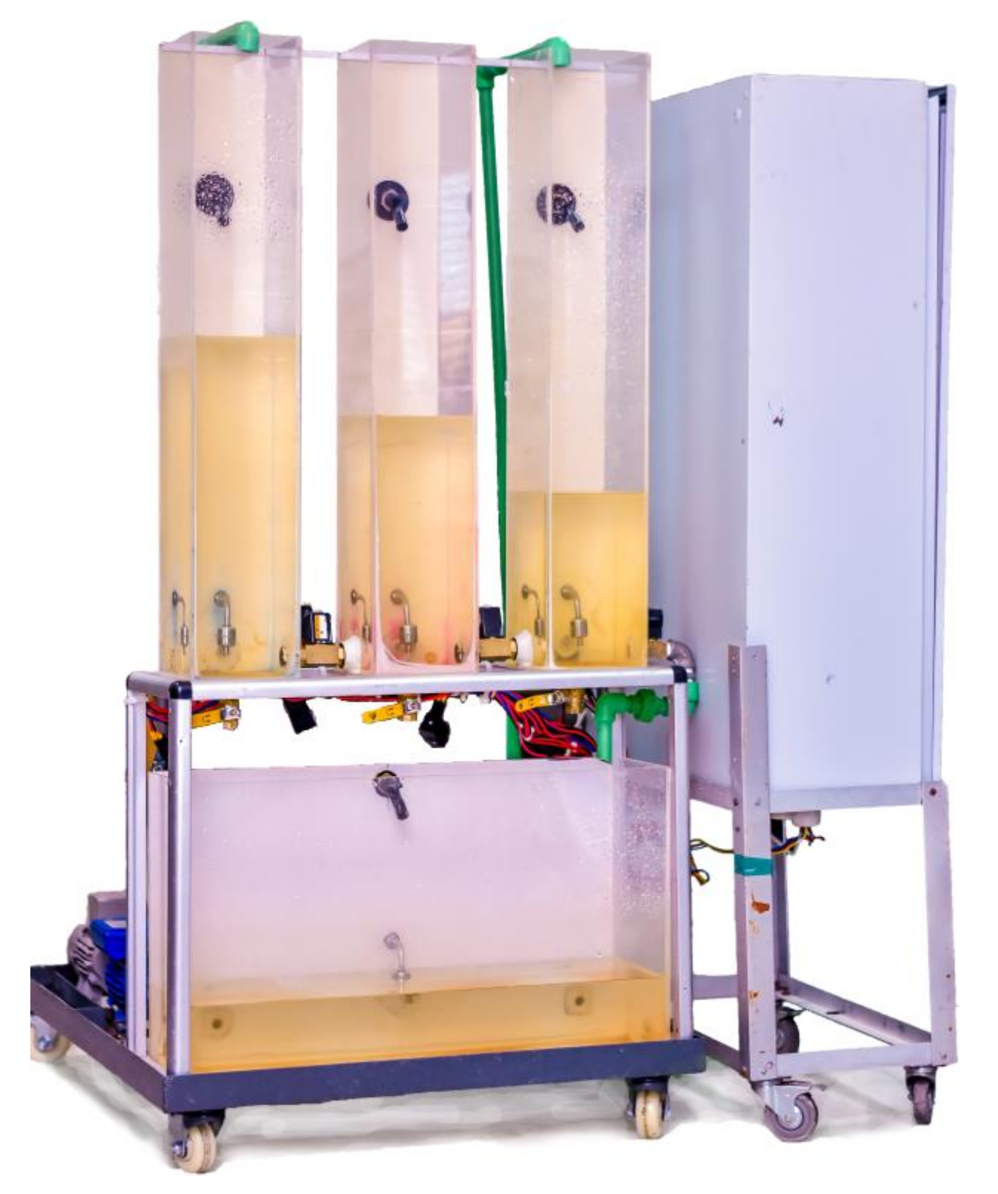
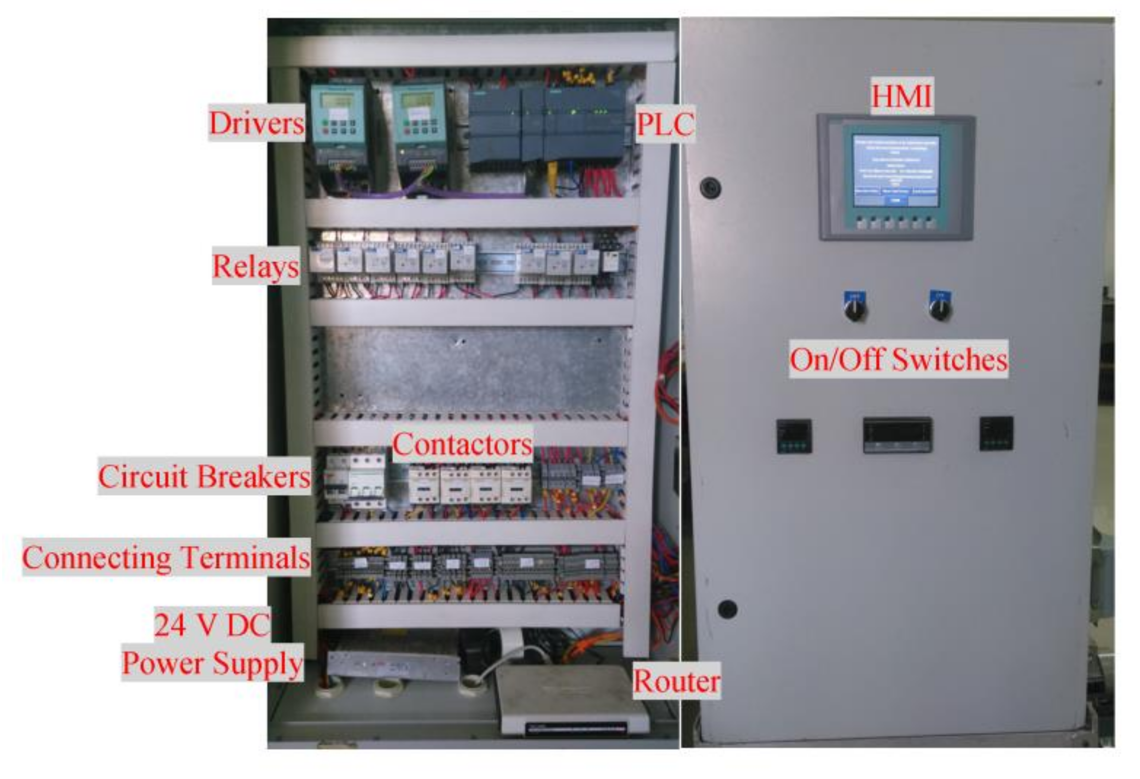
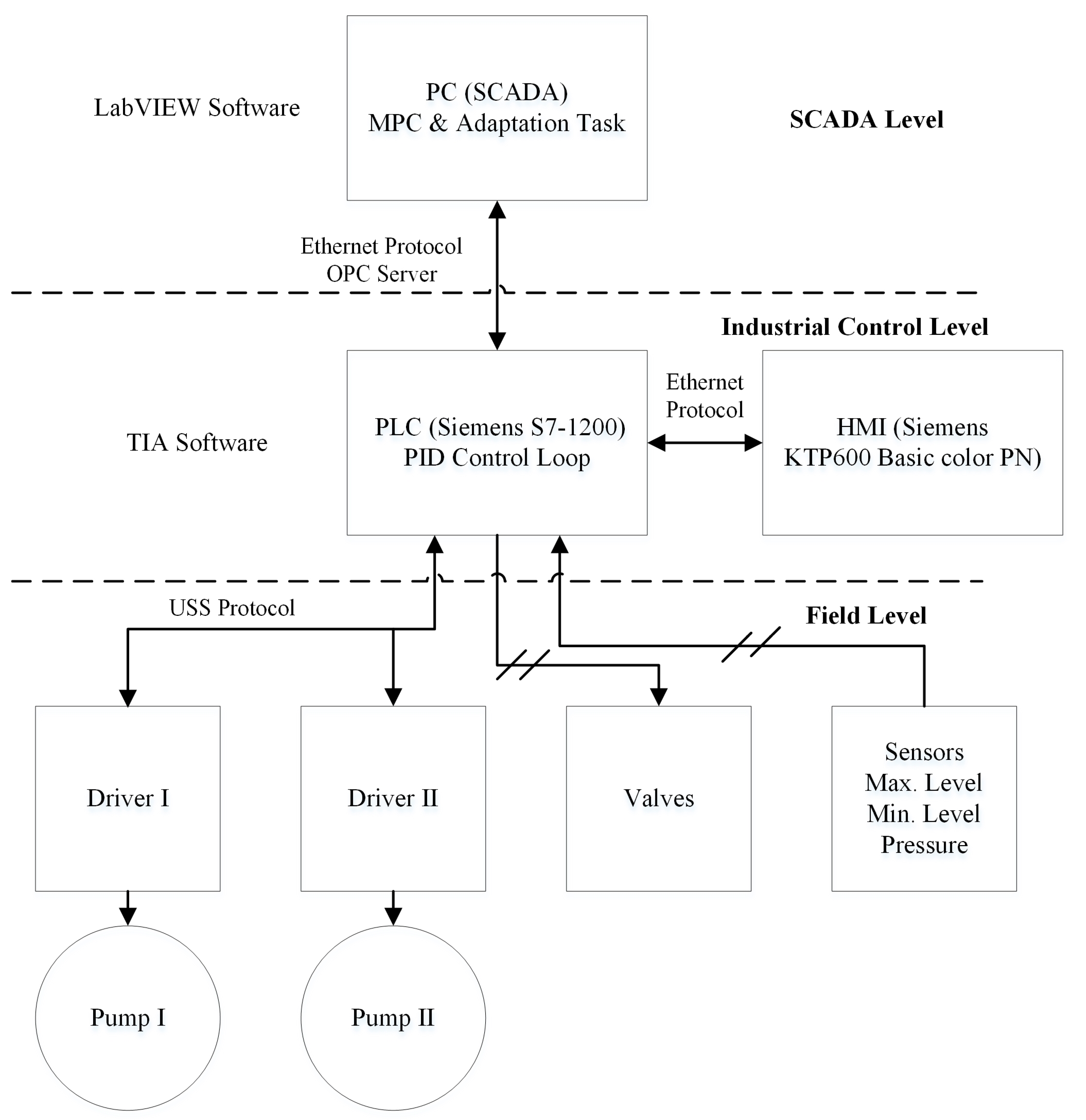
4. Experimental Work

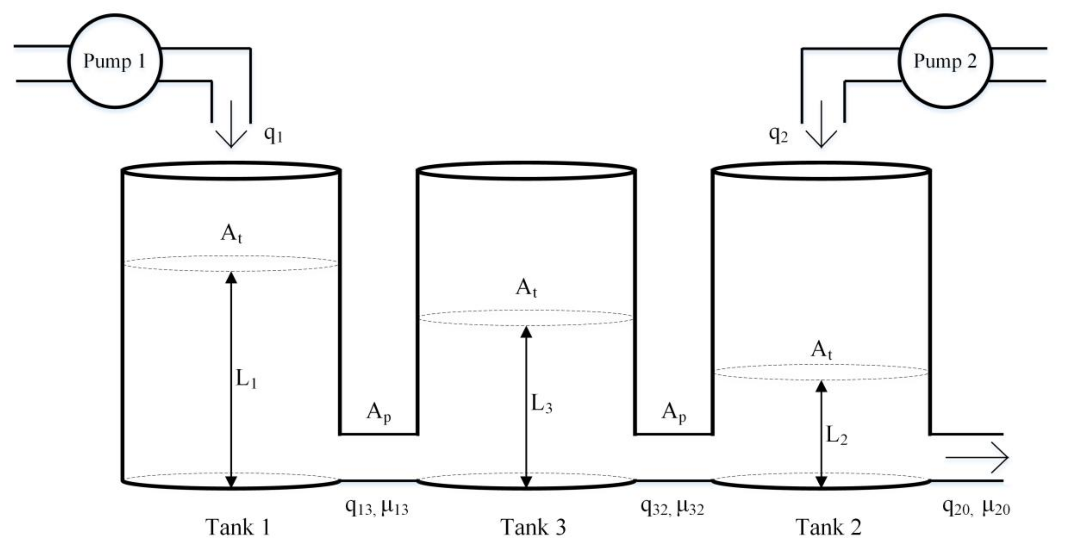
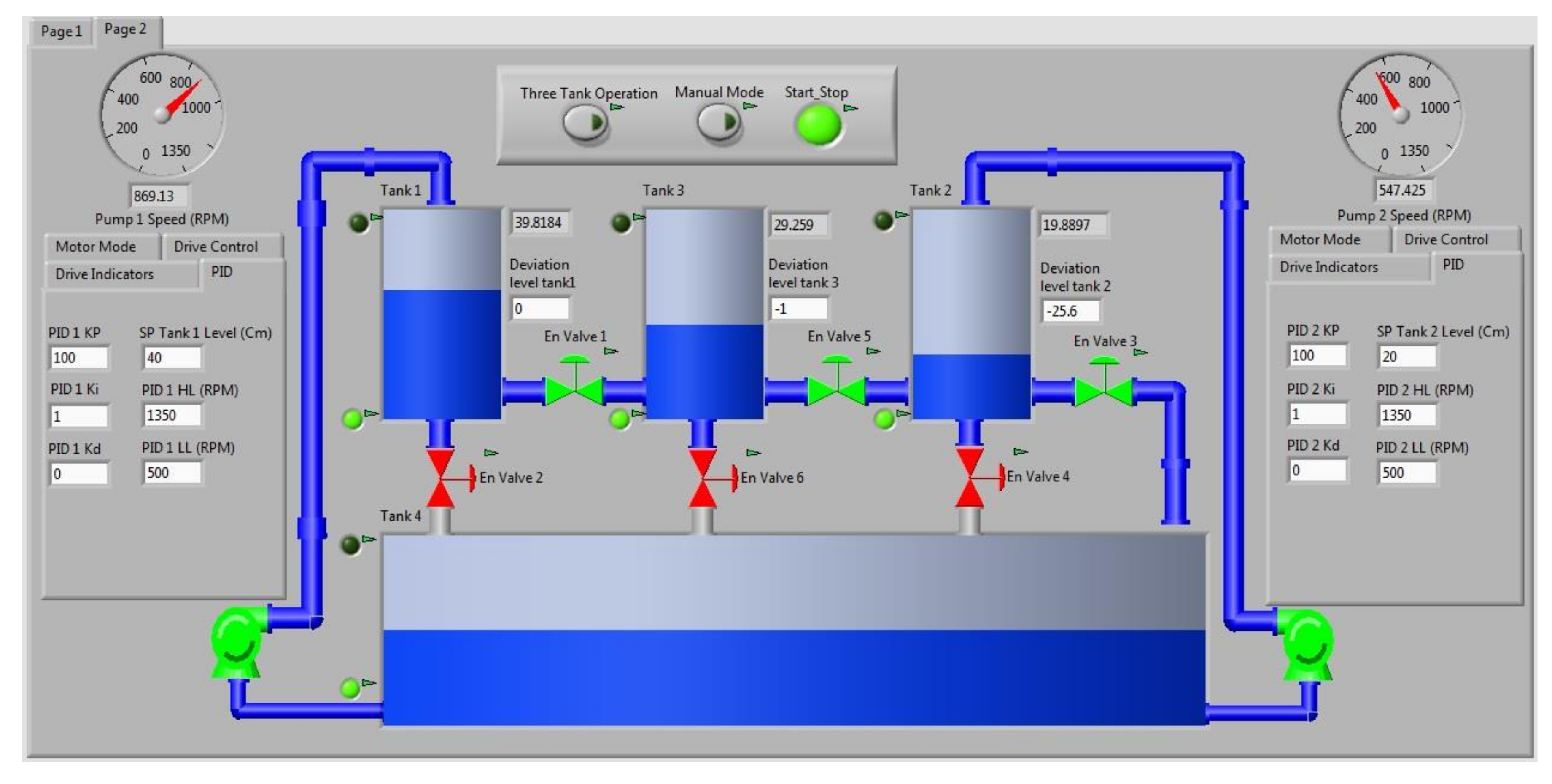
4.1. System Description
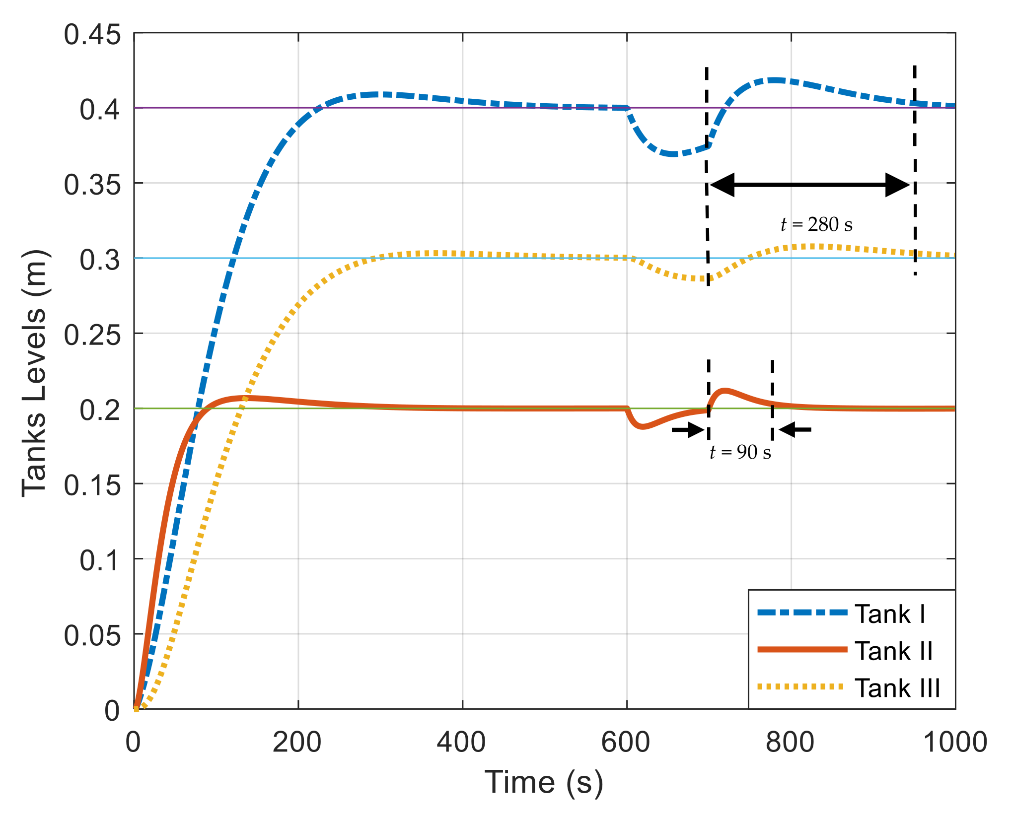
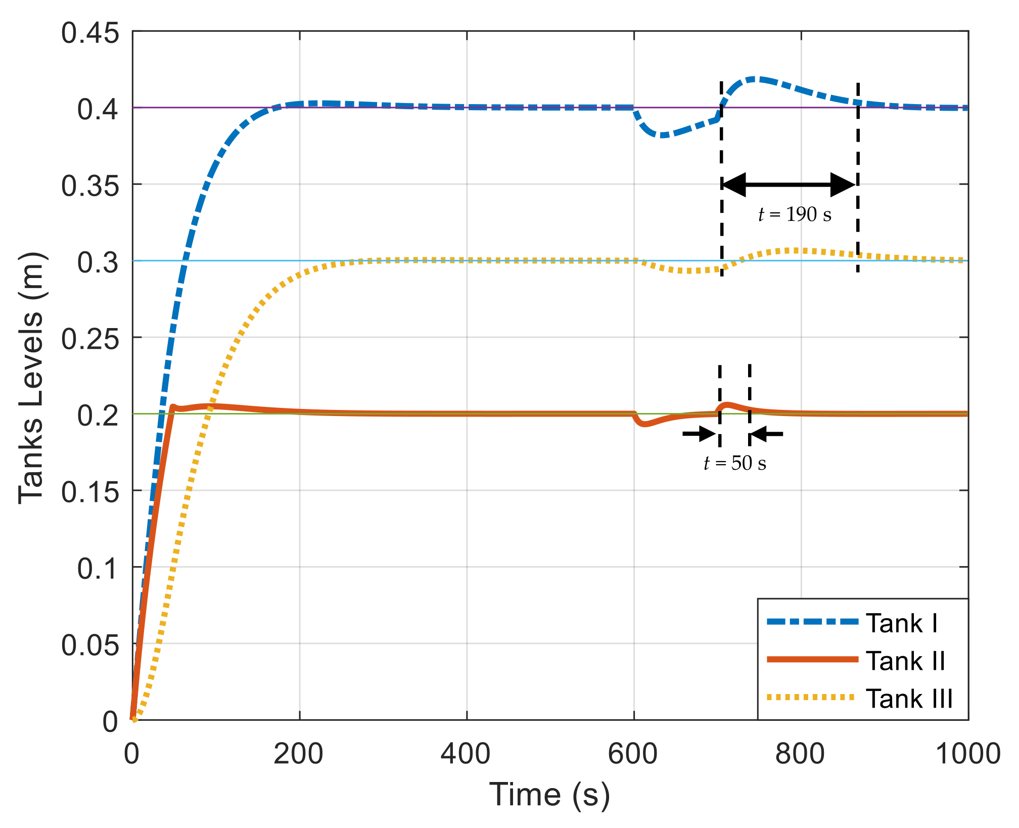
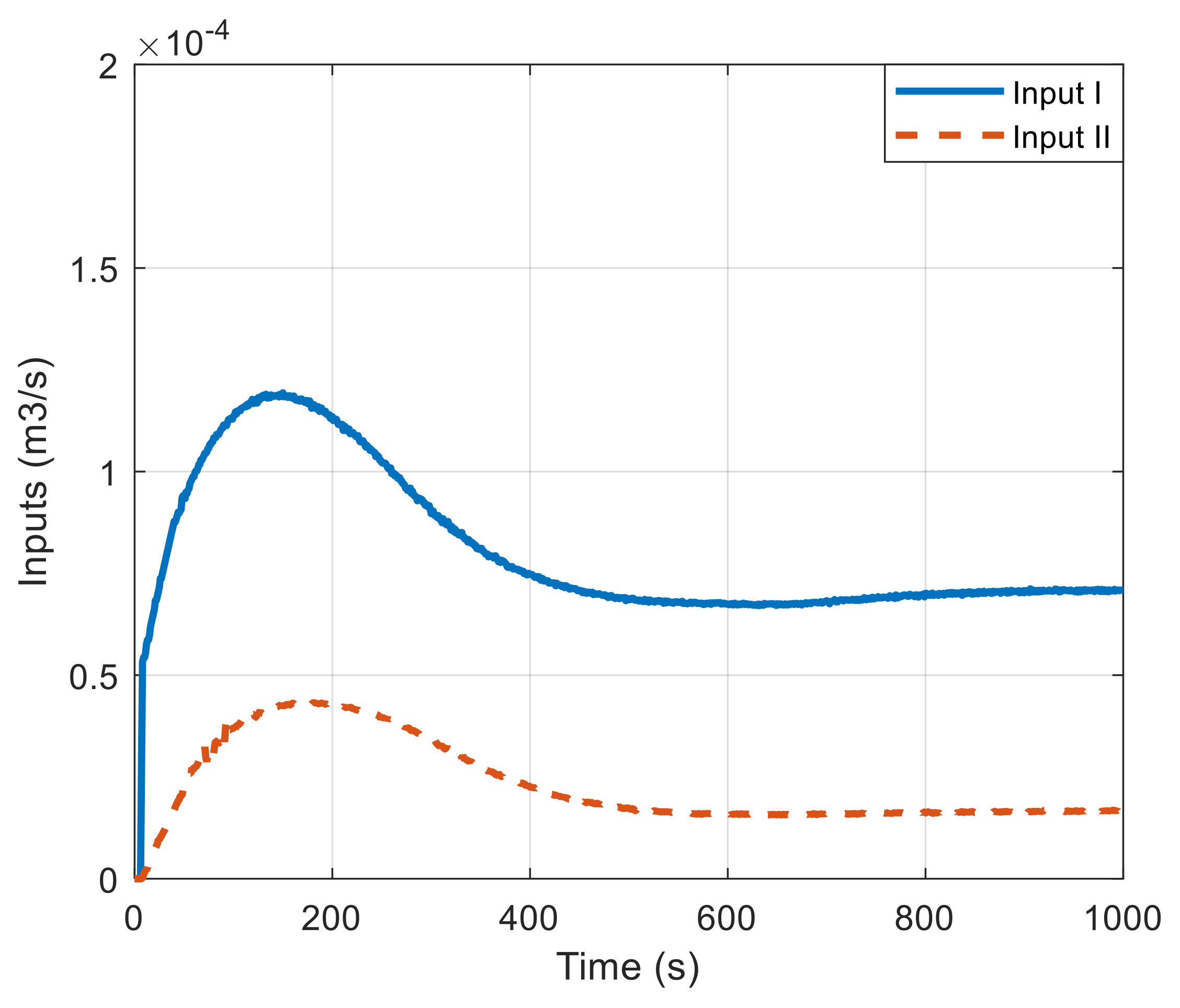
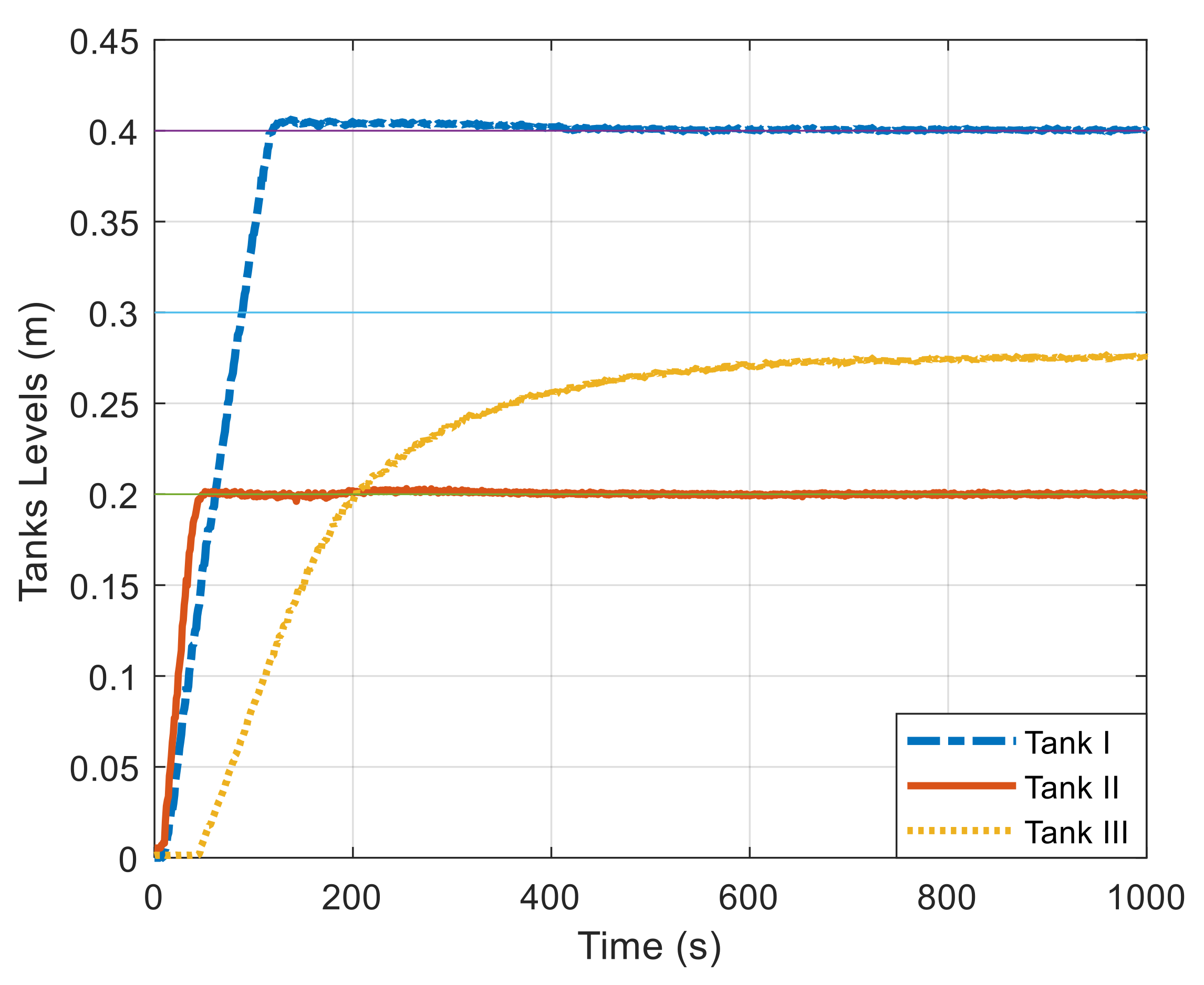
The experimental setup is represented in Figure 12. It is fully designed and implemented in the Automatic Control Laboratory of the Electrical and Control Engineering department within the AASTMT facilities. It consists of three identical square glass tanks, that is, not cylindrical as in the theoretical model. The first and second tanks are fed from the reservoir tank by two AC pumps controlled by Siemens SINAMICS G110–120 W drivers. The third tank is also connected to the first and second tanks by intermediated on/off valves. The discharge of the three tanks is controlled through an on/off valve attached to the second tank. Each tank has a manual valve to simulate the tank leakage. In addition, minimum and maximum level sensors are implemented for level safety. Moreover, a continuous level measurement for the three tanks is obtained through analogue pressure sensors. The necessary calibration process of the pressure sensors is performed.
The pump drivers are connected to the PLC through Universal Serial Interface (USS) communication protocol. USS is a serial protocol developed by Siemens Company to control its AC and DC drives. It is an access approach based on the master and slave concept for communications via a serial bus to read/write process data on the drives and to read/adjust drive parameters over the bus [43]. The relations between flow rate and pump speed, in RPM, are given by:
q 1 = 2 10 7 S p e e d 1 1 10 4   ( m 3 / s )
q 2 = 2 10 7 S p e e d 2 9 10 5   ( m 3 / s ) .
The pump’s operation could be more reliable based on [44]. As discussed earlier, the PID controller is implemented at the PLC, while its parameters are computed through the MPC controller at SCADA. Then, the parameters will be sent to the PLC through the communication network. To maintain the hierarchical control system structure, the MPC controller and the adaption task are implemented on a PC through Laboratory Virtual Instrument Engineering Workbench (Lab VIEW) software as the higher control level. Lab VIEW is a system design software and development platform used for graphical programming language from National Instruments Company. Alternatively, the PID control task is executed at Siemens PLC S7-1200 as a lower control level through Siemens Totally Integrated Automation (TIA) Software.
TIA is an engineering platform that integrates PLC controllers, HMI and motor drives in addition to other components for different automation tasks. The drives’ output voltages are applied to the motors through three-phase contactors. In case of driver’s failure, pumps can be operated directly online through interlocked contactors with the drivers’ contactors. The control cabinet is shown in Figure 13, it is equipped with Siemens KTP600 Basic color PN HMI for local system monitoring and control. The communication between PC and PLC relies on National Instruments Open Platform Communication (OPC) server through an Ethernet communication protocol. OPC is a standard interface for communicating different data sources including factories’ field devices, laboratories’ equipment and databases. Many industrial data acquisition and control devices, such as PLCs and Programmable Automation Controllers (PACs), are designed to work with the OPC foundation standard. The overall automation configuration is demonstrated in Figure 14.

4.2. Results

The experimental results have been obtained by employing Lab VIEW software. The MathScript Module has been used to develop the proposed algorithm structure through its built-in libraries and functions, for example, DCS Module, to maintain the PC SCADA system. One of the SCADA screens is shown in Figure 15. Different experiments have been carried out to obtain sufficient measurements to identify three-tank system parameters. The sampling time has been calibrated to be 1 s, while the system time constant is 48 s. After substituting by the system parameters given in Table 4, the state-space model for the experimental system is:
A = 0.9975 3.73 10 6 0.0025 3.73 10 6 0.9948 0.0029 0.0025 0.0029 0.9945 ,   B = 47.55 5.93   10 5 5.93   10 5 47.49 0.0602 0.0702 ,   C = 1 0 0 0 1 0 0 0 1 ,   D   =   0 .
Figure 16 and Figure 17 show the three-tank levels response and input flow rates of the PID controller with fixed gains, which are listed in Table 5. Figure 18 and Figure 19 represent the tank levels response and input flow rates of MPC or MPC based PID controller. MPC based PID shows a faster response for the two end tanks, the settling times are about 150 s for the first tank and 50 s for the second tank. On the other hand, the settling times for the PID controller are about 700 s for both tanks. A steady state error by 5 % of the third tank level for both controllers is observed, as it is uncontrollable state.
Additionally, no overshoots have been observed for the tank’s levels using MPC based PID controller, while for the PID controller, they are 10.9 % for the first tank and 13.3 % for the second tank. Besides, MPC based PID inputs satisfy the maximum flow rate constraints and reach the steady-state at the identified operating points in Table 4. A comparison between PID, MPC and MPC based PID for the first tank is illustrated in Table 6. The MPC calculation parameters are similar to the simulation parameters listed in Table 3, while the MPC based PID adaptable gains are illustrated in Figure 20. The RLS method requires more samples to calculate the initial experimental PID gains rather than the simulation case, so the online adaptation for PID gains started after 200 s.

5. Conclusions

The usage of automation systems and APC approaches are necessary for better performance, superior quality, and lower manufacturing costs. However, the human factor and the current automation technology should be considered during the implementation of the APC techniques. The adaptation of PID controllers for a MIMO system with constraints using an MPC controller is proposed. The proposed algorithm is executed in a hierarchical structure of two levels, one to implement PID controllers and the other to identify the PID controller gains using RLS to obtain the same performance of MPC. The proposed technique overcomes the limitation of both standalone PID and MPC controllers. It has been validated for a three-tank system as a MIMO nonlinear system with constraints. The simulation results show the effectiveness of the proposed technique. After that, it has been implemented for an experimental three-tank system setup. The experimental results show a superior transient performance of the MPC controller over the conventional PID controller without noticeable overshoot. Furthermore, MPC and MPC-based PID controllers have similar results; this reflects the effectiveness of the real implementation of the adaptation technique.

Author Contributions

Conceptualization, A.A., M.A. and E.E.Z.; methodology, A.A., M.A. and E.E.Z.; software, A.A.; validation, A.A. and M.A.; formal analysis, A.A., M.A. and E.E.Z.; writing—Original draft, A.A.; writing—Review & editing, A.A., M.A. and M.G. supervision, M.A., E.E.Z. and M.G. All authors have read and agreed to the published version of the manuscript.

Funding

This work was partly supported by the Natural Science Foundation of China through the project with code 51850410515. Also, the experimental setup was co-funded from AASTMT and EGEC Company in Egypt.

Conflicts of Interest

The authors declare no conflict of interest.

References

  1. Vandoren, V. Advances in Control Loop Optimization. Control Engineering 1 May 2008. Available online: https://www.controleng.com/articles/advances-in-control-loop-optimization (accessed on 15 July 2016).
  2. Taghizadeh, M.; Yarmohammadi, M.J. Development of a Self-tuning PID Controller on Hydraulically Actuated Stewart Platform Stabilizer with Base Excitation. Int. J. Control. Autom. Syst. 2018, 16, 2990–2999. [Google Scholar] [CrossRef]
  3. Wade, H.L. Basic and Advanced Regulatory Control: System Design and Application; ISA: Durham, NC, USA, 2017. [Google Scholar]
  4. Visioli, A. Practical PID Control; Springer Science and Business Media LLC: Berlin, Germany, 2006. [Google Scholar]
  5. Malouche, I.; Bouani, F. A New Adaptive Partially Decentralized PID Controller for Non-square Discrete-time Linear Parameter Varying Systems. Int. J. Control. Autom. Syst. 2018, 16, 1670–1680. [Google Scholar] [CrossRef]
  6. Nishikawa, Y.; Sannomiya, N.; Ohta, T.; Tanaka, H. A method for auto-tuning of PID control parameters. Automatica 1984, 20, 321–332. [Google Scholar] [CrossRef]
  7. Gyöngy, I.; Clarke, D. On the automatic tuning and adaptation of PID controllers. Control. Eng. Pract. 2006, 14, 149–163. [Google Scholar] [CrossRef]
  8. Li, M.; Zhou, P.; Zhao, Z.; Zhang, J. Two-degree-of-freedom fractional order-PID controllers design for fractional order processes with dead-time. ISA Trans. 2016, 61, 147–154. [Google Scholar] [CrossRef] [Green Version]
  9. Padula, F.; Visioli, A. Tuning rules for optimal PID and fractional-order PID controllers. J. Process. Control. 2011, 21, 69–81. [Google Scholar] [CrossRef]
  10. Begum, K.G.; Rao, A.S.; Radhakrishnan, T. Enhanced IMC based PID controller design for non-minimum phase (NMP) integrating processes with time delays. ISA Trans. 2017, 68, 223–234. [Google Scholar] [CrossRef]
  11. Wang, Q.; Lu, C.; Pan, W. IMC PID controller tuning for stable and unstable processes with time delay. Chem. Eng. Res. Des. 2016, 105, 120–129. [Google Scholar] [CrossRef]
  12. Savran, A.; Kahraman, G. A fuzzy model based adaptive PID controller design for nonlinear and uncertain processes. ISA Trans. 2014, 53, 280–288. [Google Scholar] [CrossRef]
  13. Fadaei, A.; Salahshoor, K. A novel real-time fuzzy adaptive auto-tuning scheme for cascade PID controllers. Int. J. Control. Autom. Syst. 2011, 9, 823–833. [Google Scholar] [CrossRef]
  14. Freire, H.; Oliveira, P.B.M.; Pires, E.J.S. From single to many-objective PID controller design using particle swarm optimization. Int. J. Control. Autom. Syst. 2017, 15, 918–932. [Google Scholar] [CrossRef]
  15. Chiou, J.-S.; Tsai, S.-H.; Liu, M.-T. A PSO-based adaptive fuzzy PID-controllers. Simul. Model. Pract. Theory 2012, 26, 49–59. [Google Scholar] [CrossRef]
  16. Sharma, R.; Kumar, V.; Gaur, P.; Mittal, A.P. An adaptive PID like controller using mix locally recurrent neural network for robotic manipulator with variable payload. ISA Trans. 2016, 62, 258–267. [Google Scholar] [CrossRef] [PubMed]
  17. Reynoso-Meza, G.; Carrillo-Ahumada, J.; Boada, Y.; Picó, J. PID controller tuning for unstable processes using a multi-objective optimisation design procedure. Ifac-Pap. 2016, 49, 284–289. [Google Scholar] [CrossRef]
  18. Lu, K.; Zhou, W.; Zeng, G.; Du, W. Design of PID controller based on a self-adaptive state-space predictive functional control using extremal optimization method. J. Frankl. Inst. 2018, 355, 2197–2220. [Google Scholar] [CrossRef]
  19. Çetin, M.; Iplikci, S. A novel auto-tuning PID control mechanism for nonlinear systems. ISA Trans. 2015, 58, 292–308. [Google Scholar] [CrossRef]
  20. Agarwal, R. How Advanced Process Control Lowers Cost and Enhances Industrial Production Efficiency; Schneider Electric: Rueil-Malmaison, France, 2014. [Google Scholar]
  21. Mehta, B.R.; Reddy, Y.J. Chapter 1—Industrial automation. In Industrial Process Automation Systems; Mehta, B.R., Reddy, Y.J., Eds.; Butterworth-Heinemann: Oxford, UK, 2015; pp. 1–36. [Google Scholar]
  22. Omer, A.I.; Taleb, M.M. Architecture of Industrial Automation Systems. Eur. Sci. J. 2014, 10, 273–283. [Google Scholar]
  23. Agundis-Tinajero, G.; Segundo-Ramírez, J.; Visairo-Cruz, N.; Savaghebi, M.; Guerrero, J.M.; Barocio, E. Power flow modeling of islanded AC microgrids with hierarchical control. Int. J. Electr. Power Energy Syst. 2019, 105, 28–36. [Google Scholar] [CrossRef] [Green Version]
  24. Chen, Y.; Qin, J.-C.; Dong, Z.-Y.; Liu, S.-A.; Zheng, H.-L. Multilayer hierarchical control for robotic coax-helicopter based on the H∞ robustness and mixing control scheme. Adv. Mech. Eng. 2017, 9, 1687814017720088. [Google Scholar] [CrossRef]
  25. Abd-Elgeliel, M.; Badreddin, E.; Gambier, A. Application of model predictive control for fault tolerant system using dynamic safety margin. In Proceedings of the 2006 American Control Conference, Minneapolis, MN, USA, 14–16 June 2006; p. 6. [Google Scholar]
  26. Zhang, J.; Yang, H.; Li, M.; Wang, Q. Robust Model Predictive Control for Uncertain Positive Time-delay Systems. Int. J. Control. Autom. Syst. 2019, 17, 307–318. [Google Scholar] [CrossRef]
  27. Lee, J.H. Model predictive control: Review of the three decades of development. Int. J. Control. Autom. Syst. 2011, 9, 415–424. [Google Scholar] [CrossRef]
  28. Huang, Z.; Yang, T.; Giangrande, P.; Galea, M.; Garcia, C.; Rivera, M.; Wheeler, P.; Rodriguez, J. Voltage Utilization Enhancement of Dual Inverters by Model Predictive Control for Motor Drive Applications. In Proceedings of the IEEE International Symposium on Predictive Control of Electrical Drives and Power Electronics (PRECEDE), Quanzhou, China, 31 May–2 June 2019; pp. 1–3. [Google Scholar] [CrossRef]
  29. Afram, A.; Janabi-Sharifi, F. Supervisory model predictive controller (MPC) for residential HVAC systems: Implementation and experimentation on archetype sustainable house in Toronto. Energy Build. 2017, 154, 268–282. [Google Scholar] [CrossRef]
  30. Riverso, S.; Mancini, S.; Sarzo, F.; Ferrari-Trecate, G. Model Predictive Controllers for Reduction of Mechanical Fatigue in Wind Farms. IEEE Trans. Control. Syst. Technol. 2016, 25, 535–549. [Google Scholar] [CrossRef] [Green Version]
  31. Ouammi, A.; Achour, Y.; Zejli, D.; Dagdougui, H. Supervisory Model Predictive Control for Optimal Energy Management of Networked Smart Greenhouses Integrated Microgrid. IEEE Trans. Autom. Sci. Eng. 2020, 17, 117–127. [Google Scholar] [CrossRef]
  32. Sato, T. Design of a GPC-based PID controller for controlling a weigh feeder. Control. Eng. Pract. 2010, 18, 105–113. [Google Scholar] [CrossRef]
  33. Xu, M.; Li, S.; Qi, C.; Cai, W. Auto-tuning of PID controller parameters with supervised receding horizon optimization. ISA Trans. 2005, 44, 491–500. [Google Scholar] [CrossRef]
  34. Kubalčik, M.; Bobál, V. Adaptive control of three tank system: Comparison of two methods. In Proceedings of the 16th Mediterranean Conference on Control and Automation, Ajaccio, France, 25–27 June 2008; pp. 1041–1046. [Google Scholar]
  35. Abdelrauf, A.A.; Abdel-Geliel, M.; Zakzouk, E. Adaptive PID controller based on model predictive control. In Proceedings of the 2016 European Control Conference (ECC), Aalborg, Denmark, 29 June–1 July 2016; pp. 746–751. [Google Scholar]
  36. Abdelrauf, A.A.; Saad, W.W.; Hebala, A.; Galea, M. Model Predictive Control Based PID Controller for PMSM for Propulsion Systems. In Proceedings of the 2018 IEEE International Conference on Electrical Systems for Aircraft, Railway, Ship Propulsion and Road Vehicles & International Transportation Electrification Conference (ESARS-ITEC), Nottingham, UK, 7–9 November 2018; pp. 1–7. [Google Scholar]
  37. Maciejowski, J.M. Predictive Control: With Constraints; Prentice Hall: Upper Saddle River, NJ, USA, 2002. [Google Scholar]
  38. Zhao, K.; Lü, X.; Zheng, W.; Huang, C. Direct relaxation of hard-constraint in Model Predictive Control. In Proceedings of the 2012 9th International Conference on Fuzzy Systems and Knowledge Discovery, Sichuan, China, 29–31 May 2012; pp. 2366–2370. [Google Scholar]
  39. Li, Y.; Liu, J.; Wang, Y. Design approach of weighting matrices for LQR based on multi-objective evolution algorithm. In Proceedings of the 2008 International Conference on Information and Automation, Changsha, China, 20–23 June 2008; pp. 1188–1192. [Google Scholar]
  40. Ikonen, E.; Najim, K. Advanced Process Identification and Control; Informa UK Limited: London, UK, 2001. [Google Scholar]
  41. Noura, H.; Theilliol, D.; Ponsart, J.C.; Chamseddine, A. Fault-Tolerant Control Systems: Design and Practical Applications; Springer: London, UK, 2009. [Google Scholar]
  42. Åström, K.J.; Hägglund, T. Advanced PID Control; ISA-The Instrumentation, Systems, and Automation Society: Pittsburg, PA, USA, 2006. [Google Scholar]
  43. Möller-Nehring, W.; Bohrer, W. Universal Serial Interface Protocol USS Protocol; Siemens Company: Munich, Germany, 1994. [Google Scholar]
  44. Galea, M.; Giangrande, P.; Madonna, V.; Buticchi, G. Reliability-Oriented Design of Electrical Machines: The Design Process for Machines’ Insulation Systems MUST Evolve. IEEE Ind. Electron. Mag. 2020, 14, 20–28. [Google Scholar] [CrossRef]
Figure 1. Advanced Process Control (APC) Factors.
Energies 13 06594 g001
Figure 2. Hierarchical control for the proposed technique.
Energies 13 06594 g002
Figure 3. General representation of the cascade controller for Multi-Input Multi-Output (MIMO) system feedback control.
Energies 13 06594 g003
Figure 4. The proposed algorithm structure.
Energies 13 06594 g004
Figure 5. The proposed algorithm flow chart.
Energies 13 06594 g005
Figure 6. Three tank system.
Energies 13 06594 g006
Figure 7. System response using fixed PID controller.
Energies 13 06594 g007
Figure 8. Input flow rates using fixed PID controller.
Energies 13 06594 g008
Figure 9. System response using MPC based PID controller.
Energies 13 06594 g009
Figure 10. Input flow rates using MPC based PID controller.
Energies 13 06594 g010
Figure 11. Adaptive gains of PID controller (a) KP, (b) KI and (c) KD.
Energies 13 06594 g011aEnergies 13 06594 g011b
Figure 12. Three tank system experimental setup.
Energies 13 06594 g012
Figure 13. Three tank system control cabinet.
Energies 13 06594 g013
Figure 14. Three tank system automation levels configuration.
Energies 13 06594 g014
Figure 15. PC SCADA system.
Energies 13 06594 g015
Figure 16. Experimental setup levels’ response using fixed PID controller.
Energies 13 06594 g016
Figure 17. Experimental setup input flow rates using fixed PID controller.
Energies 13 06594 g017
Figure 18. Experimental setup levels’ response using MPC based PID controller.
Energies 13 06594 g018
Figure 19. Experimental setup input flow rates using MPC based PID controller.
Energies 13 06594 g019
Figure 20. Experimental adaptable gains of (a) PID I and (b) PID II.
Energies 13 06594 g020
Table 1. Three tank system parameters.
Tank cross section area (At)0.0154 m2
Pipe cross-section area (Ap)5 × 10⁻⁵ m2
Outflow coefficient (µmn)µ13 = 0.5, µ32 = 0.5, µ20 = 0.675
Maximum flow rate constraint (Qmax)1.2 × 10⁻⁴ m3/s
Maximum level (Lmax)0.62 m
Operating pointQ1 = 0.35 × 10⁻⁴ m3/s, Q2 = 0.375 × 10⁻⁴ m3/s
L10 = 0.4 m, L20 = 0.2 m, L30 = 0.3 m
Table 2. PID fixed gains.
PID IPID II
KP4.29×10−4KP10.83 × 10−4
KI5.32 × 10−6KI3.94 × 10−5
KD−1.42 × 10⁻⁴KD−13.51 × 10⁻⁴
Table 3. The simulation data.
Prediction horizon (ny)10
Control horizon (nu)10
Sampling time (Ts)1 s
Table 4. Experimental three-tank system parameters.
Tank cross-section area (At)0.021 m2
Pipe cross-section area (Ap)1.26677 × 10⁻⁴ m2
Outflow coefficients (µmn) µ 13 = 0.06
µ 32 = 0.07
µ 20 = 0.074
Maximum flow rates (Qmax)Q1 = 1.7 × 10⁻⁴ m3/s (1350 RPM)
Q2 = 1.8 × 10⁻⁴ m3/s (1350 RPM)
Maximum level (Lmax)0.65 m
Operating points q 1 = 7.5 × 10⁻⁵ m3/s (875 RPM)
q 2 = 1.7 × 10⁻⁵ m3/s (535 RPM)
L10= 0.4 m
L20= 0.2 m
L30= 0.3 m
Table 5. Experimental PID fixed gains.
PID IPID II
KP100KP100
KI1KI1
KD10KD10
Table 6. Comparison of different control configuration results.
ControllerPIDMPCMPC Based PID
Criteria
PerformanceSettling Time (s)700150150
Overshoot %10.900
RealizationSimple & centralized in PLCDifficult & centralized in SCADASimple & distributed in PLC and SCADA
ConstraintsNot applicableEasy to handleEasy to handle
Sampling timeLowHighLow
Publisher’s Note: MDPI stays neutral with regard to jurisdictional claims in published maps and institutional affiliations.

