Abstract
The combined cooling, heating, and power (CCHP) microgrid system is good for energy gradient utility. At the same time, it can promote the renewable energy (RE) consumption and abate environmental pollution. In a CCHP microgrid system, the electrical energy storage (EES), which can storage and release electrical energy, plays an indispensable role. A robust optimization model of the CCHP microgrid participating in power market transaction is constructed to calculate the CCHP microgrid operation cost in 4 cases. The results show that the EES can significantly reduce the cost of the CCHP microgrid by 13.21%, compared with 8.36% in Group 1 without renewable energy. The EES can reduce the reserved capacity of micro gas turbine units to deal with the precariousness of RE generation and then reduce the CCHP microgrid operation cost by reducing the purchase of energy from the power grid and arbitrage. Finally, the calculation method of comprehensive value of the EES is constructed. The comprehensive value of the EES is higher in Group 2 with renewable energy compared with Group 1 without renewable energy. Through net present value (NPV) calculation and sensitivity analysis, it is found that the RE penetration level and EES cost have the greatest impact on the economic performance of EES. This shows that with the continuous rising of the RE penetration level and the gradual decrease of EES cost, great potential still waits to be tapped in the comprehensive value of EES in the future.
1. Introduction
With the global climate deterioration and energy consumption crisis becoming increasingly obvious, the clean and efficient use of energy has become a focus recently [1]. The growth and efficient use of renewable energy (RE) has become an essential part of the energy strategy of many countries. According to the data released by the International Renewable Energy Agency (IRENA) in 2020, by the end of 2019, the cumulative installed capacity of global RE was 2537 GW [2]. The newly installed capacity was 176 GW [3], with a year-on-year increase of 7.9% [3], of which the total newly installed capacity of wind and solar energy accounted for 90% [3]. However, the RE output has the attributes of fluctuation and randomness [4]. When extensive accessing to the power grid, the renewable energy may threaten the security and stability of the power grid. In addition, such as curvature condition of wind power and photovoltaic power will result in invalid investment problems [5].
A combined cooling, heating, and power (CCHP) microgrid system is an integrated energy system which combines load, energy equipment, RE, natural gas, electric power, and other energy [6,7,8]. The CCHP microgrid system is good for energy gradient utility. At the same time, it can promote the RE consumption and abate environmental pollution [9]. In a CCHP microgrid system, the electrical energy storage system, which can storage and release energy, plays an indispensable role. Its extremely strong flexibility can instantly stabilize the impact of the randomness of renewable energy generation on the CCHP microgrid system [10]. While promoting renewable energy consumption, electrical energy storage access to a CCHP microgrid can also increase the stability of the CCHP microgrid operation, optimize the operation status of conventional units, reduce dependence on the main grid, and reduce environmental pollution caused by emissions [11]. Therefore, the comprehensive value of electrical energy storage discussed in this paper is the stacking revenues which can reduce the system cost when it is connected to a CCHP microgrid. The comprehensive value of electrical energy storage includes arbitrage value brought by charging and discharging to help renewable energy consumption, increasing the stability of CCHP microgrid operation, cutting the transaction cost of power energy from the main grid and environmental value brought by emission reduction. At present, the electrical energy storage power station can only obtain arbitrage revenue, which generally cannot cover its extremely high investment cost, and its economic performance is poor [12]. Therefore, it is urgent to calculate the value of electrical energy storage in practical application, so as to provide reference for pricing energy storage services and formulating incentive compensation policies in the power market.
The relevant research on energy storage value calculation first appeared in the research on improving the security and stability of energy storage equipment connected to the power system [13]. The optimization objectives of related research can be divided into two categories: economy and security. However, at that time, energy storage is not considered as an independent subject in the power system, only the change of optimization constraints after considering its technical characteristics [14,15,16]. The economics of energy storage are not the main research issues. In the case of power and capacity of energy storage determined, the current research on the value of energy storage can be divided into the following three categories: (1) Considering the technical and economical performance of energy storage equipment, the comprehensive evaluation of different types of energy storage is carried out. The relevant scholars have comprehensively considered such indicators as maximum charge and discharge efficiency [17], self discharge rate [17], capacity cost [18], energy storage system profile [18], energy saving and emission reduction efficiency [19], and the like. (2) The whole life cycle technical and economical study of energy storage is carried out. Some researchers use the financial analysis method of net present value (NPV) [20], investment payback period [21], and other indicators to study this problem. Some scholars use the methods of life cycle cost of storage (LCCOS) and leveled cost of energy (LCOE) [22] and cost-benefit analysis [23] to analyze and evaluate the economic performance of energy storage in a long time scale from the perspective of investors. (3) Study the single value of energy storage in a certain scenario. Khastieva D (2019) proposes a mathematical model of incorporating regulatory constraints into commercial regulatory investment planning [24]. In IEEE 118 bus system, the case study of 6-node shows that energy storage investment is a supplement to transmission expansion and helps to improve social welfare value. The potential application of a typical South Norwegian house with BIPV system for on-site battery energy storage was studied in Ref. [25]. The results show that such a system has better techno-economical performance than its counterpart. Ogland-Hand J D (2019) separately investigate the value that the bulk energy storage (BES) system can reduce the carbon dioxide emission and water demand of the whole system [26]. According to the characteristics of net load, BES technology and the price of carbon dioxide and water, the operation of BES can not only improve the utilization rate of traditional energy generation capacity, but also improve the utilization rate of renewable energy generation capacity.
Considering there are few researches on the quantitative calculation of energy storage value at present, most of the related research on energy storage value is single value measurement of energy storage and focus on the whole life cycle analysis with a long time scale. The future energy storage technology, cost, and benefit are uncertain, so it is essential to study comprehensive value of electrical energy storage application in a shorter time scale combined with the current new application scenarios of energy storage. At present, a large number of researchers have studied the energy storage application effect when energy storage is combined with the operation of the microgrid system with multi energy. Ref. [27] proposed a microgrid to participate in a day-ahead market operation optimization strategy considering demand response (DR). When implementing DR, the microgrid operation cost dropped by 4.17%. Sensitivity analysis results reveal that the microgrid operation cost drops with the raise of the energy storage capacity. In order to keep the conservatism and computational complexity at a low level, a stochastic-robust coordinated optimization model for the CCHP micro-grid considering multi-energy operation and power trading is proposed in Ref. [28] by combining stochastic optimization and robust optimization methods. The numerical results show the effectiveness of the proposed stochastic-robust method, and find that the energy storage system plays an important role in the CCHP microgrid. Ref. [29] proposed a novel operation model which called the Wasserstein-based two-stage distributional robust optimization (WTSDRO) for the CCHP microgrid participation in the day-ahead marked. The results show that due to the existence of flexible resources such as the energy storage system and demand response, the operation cost and carbon dioxide emission of the whole system will be further reduced after reasonable scheduling. Ref. [30] proposed a piecewise least squares linearization method. The results show that the standard error of the performance curve can be reduced by at least 20.97% compared with the segment broken-line linearization method. Compared with the least square linearization method, the standard error of the performance curve can be reduced by at least 75.49%.
In terms of solving methods, some scholars generate random scenarios of wind power output through uncertain probability density functions and use the stochastic optimization algorithm to calculate the optimal operation strategy [27,31,32]. Some scholars reduce the generated random scenarios and then use the piecewise linearization method [33] or directly use the intelligent algorithm to solve the problem [34,35]. Some scholars use the robust optimization algorithm to solve the problem [28,29]. A stochastic optimization method is established based on scenarios by many scholars [27,31,32]. When there are too few scenes, the expression of uncertainty will be distorted. If there are too many scenes, the efficiency of solving the model will be affected. The robust optimization algorithm has the advantages of no need of accurate probability distribution information of uncertain parameters and fast calculation. It has unique advantages in solving the uncertainty problem introduced by the CCHP microgrid system with high complexity [29]. Especially, the effective construction of uncertainty of wind and photovoltaic RE helps to improve the accuracy of energy storage value calculation.
A robust optimization model of the CCHP microgrid participating in power market transaction is constructed to calculate the comprehensive value of electrical energy storage in this article. In this context, the innovation points are as follows:
- (1)
- The uncertainty set of wind power and photovoltaic output is constructed to solve the problem that wind power is difficult to accurately predict. Based on the uncertainty set, the CCHP microgrid operation optimization model, including renewable energy and electrical energy storage, is transformed into a two-stage robust optimization model. This method could significantly increase the accuracy of energy storage value measurement by handling the volatility of RE in the CCHP microgrid.
- (2)
- This paper focuses on the comprehensive value of energy storage equipment in the CCHP microgrid participating in power market transactions, including the impact of the operation cost of the CCHP microgrid, the cost of trading energy with the main grid (MG), the micro gas turbine units generation, the consumption of renewable energy, and reduction of emission. The results can provide a reference for the pricing of energy storage services and the making of incentive compensation policies.
- (3)
- In this paper, a typical CCHP microgrid system with electrical energy storage is constructed to test the two-stage robust optimization model feasibility of the comprehensive value calculation of electrical energy storage in the CCHP microgrid with RE.
The rest of the article is structured as follows: Section 2 establishes the CCHP microgrid model with electrical energy storage and renewable energy. In Section 3, firstly, the mathematical model of the CCHP microgrid unit is constructed. Secondly, a two-stage robust optimization model of the CCHP microgrid is constructed by building the uncertainty set of wind power and photovoltaic power. Finally, the solution method is given. Section 4 shows the simulation data, analyzes and discusses the simulation results, and makes a sensitivity analysis. Finally, the conclusion is in Section 5.
2. CCHP Microgrid Model
The structure of the CCHP microgrid system with renewable energy and energy storage is shown in Figure 1. The CCHP microgrid units of the CCHP microgrid includes micro gas turbine, wind turbine, solar PV unit, electrical energy storage system, gas-fired boiler, heat recovery device, absorption chiller, and electric chiller. Each unit operates in coordination to satisfy the demand of power, cooling, and heat load. In the Figure 1, different colors represent different energy flows in the CCHP microgrid, and the arrows represent the flow direction of energy. For example, yellow represents natural gas, green represents power, red represents thermal power, and blue represents cold power. The CCHP microgrid can participate in the power market. Therefore, the bidirectional arrow is used to indicate that power flows between the MG and the CCHP microgrid, and the unidirectional arrow indicates that natural gas can only be purchased by the CCHP microgrid.
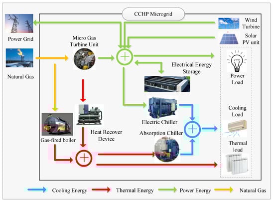
Figure 1.
The combined cooling, heating, and power (CCHP) microgrid architecture.
3. Problem Formulation
3.1. Mathematical Model of the CCHP Microgrid Units
Mathematical model of each unit of the CCHP microgrid is as follows:
3.1.1. Micro Gas Turbine Units
Micro-gas turbine (MT) units operating cost during the time period is as follows:
where indicates the natural gas price purchased by the CCHP microgrid; presents the generation efficiency of the MT; and indicate the generation power and natural gas consumption of the MT at time ; accounts for natural gas heat-value.
Accordingly, the thermal power output of the MT at time is as follows:
where and demonstrate the heat loss rate and energy efficiency coefficient of the MT.
3.1.2. Wind Turbine
The wind turbine (WT) generation is primarily determined by wind speed, the correlation between wind speed and WT output is discussed in Ref. [36]. The functional relationship is:
where indicates the wind turbine output power at time ; presents wind speed at time ; and indicate the cut in and cut out wind speed of WT; and account for output power and rated wind speed of WT.
3.1.3. Solar PV Units
The solar PV units generation mainly depends on the intensity of light radiation. The model of solar PV units generation is discussed in Ref. [37], and the functional relationship is:
where is solar PV units generation at time ; and represent the light intensity and the angle of light incident on the photovoltaic panels; and demonstrate the conversion efficiency and area of the photovoltaic panels.
3.1.4. Gas-Fired Boiler
The operating cost of the gas-fired boiler (GB) during the time period is:
where is energy efficiency coefficient of the GB; and indicate the output thermal power and natural gas consumption of the GB.
3.1.5. Heat Recover Device
The heat recovery device (HR) recovers heat power from the MT at time is as follows:
where is the heat recovery efficiency of the HR.
3.1.6. Electrical Energy Storage
Because the timescale chosen in this paper is daily date, , which indicates reasonable initial residual energy of electrical energy storage (EES) is given in the operation scheduling. The residual energy of the EES is still , after charging and discharging operation of EES at the end of one day. This method not only improves the efficiency of solving the model, but also ensures the continuity of the calculation results in time [27].
The relation between residual energy and charging power and discharging power of the EES during the time period is as follows:
where and indicate charging and discharging efficiency of EES; and present the energy loss rate and power energy loss of the EES at time . Equation (8) represents the natural energy loss of EES under actual working condition state.
The operating cost of the EES during the time period is as follows:
where is the unit operating cost of the EES at time . It should be noted that the origin of power energy acquired by the EES when the EES is charging power cannot be determined at time . So, the cost of power energy during the charging period cannot be distinguished by the supply source of the power energy. Therefore, this article introduces opportunity cost to solve this matter. If the CCHP microgrid operator starts charging the EES at time , he will give up the income of selling this part of power energy to the power market at the market price at time . Therefore, this paper considers that the cost of the power energy is power price of market at time .
3.1.7. Absorption Chiller and Electric Chiller
Mathematical formulas about energy output and input of the absorption chiller (AC) and the electric chiller (EC) are as follows:
where and are the cooling output power and heat input power of AC at time ; and account for the cooling output power and electric input power of the EC at time ; and indicate the energy efficiency coefficients of the AC and the EC, respectively.
3.1.8. The Transaction of Power Energy from MG
The transaction cost of power energy between the CCHP microgrid and MG is:
where is the market price of power energy of the MG at time ; presents the CCHP microgrid trading power energy with MG at time . When , it means the CCHP microgrid purchasing power energy from MG at time . When , it means the CCHP microgrid selling power energy to MG at time .
3.2. CCHP Microgrid Two-Stage Robust Optimization Model
The CCHP microgrid can meet the demand of users for cooling, thermal and electric energy through the integrated energy supply system, so as to improve the energy utilization efficiency. As an integrated energy system with high flexibility, the CCHP microgrid can also optimize the next day’s microgrid operation and scheduling by using the historical data of market power price, cooling, thermal and power load, wind turbine and solar PV unit output. In this article, the CCHP microgrid is connected to the grid. It sells power energy to the main grid when the energy over supplies, and purchases energy from the main grid when power supply is insufficient.
3.2.1. Hypothetical Conditions
On the premise of generality, for the sake of facilitate the calculation, the assumptions put forward in this article are as follows:
- (1)
- The security constraints within the CCHP microgrid energy network have been solved and the grid loss within the CCHP microgrid is ignored as well.
- (2)
- The marginal cost of WT and solar PV unit power generation is 0.
- (3)
- The CCHP microgrid is the price taker when it participates in power market. Therefore, the CCHP microgrid operation strategy in this market will not have an influence on clearing price of power market.
3.2.2. Uncertainty Modeling
When the CCHP microgrid participates in the day-ahead market, it is necessary to declare the trading plan of the next day in advance. However, because of stochastic fluctuation of the WT and PV generation, the actual trading power of the next day will deviate from the previous declaration. In this paper, the uncertainty characteristics of the wind and photovoltaic power are described by establishing the uncertainty sets. Based on the uncertainty sets, the CCHP microgrid robust optimization scheduling model is established, which can make the optimization results more realistic and the energy storage value calculated more accurate.
- (1)
- Uncertainty set of WT generation
For the sake of building the uncertainty set of WT generation, it is important to analyze the historical data of WT generation [38]. According to the method of reference [38], after selecting a continuous range that can cover all scenarios of WT generation in the selected time period, the corresponding uncertainty can be expressed by the uncertainty set with certain radius constraint as follows:
- (2)
- Uncertainty set of solar PV units generation
Similarly, the uncertainty set of solar PV units generation is established as follows:
where and are the uncertainty sets of WT and solar PV units generation; and represents the actual WT and solar PV units generation; , , , and indicate the minimum and maximum limits of wind turbine and solar PV unit output at time respectively; is the number of time periods in a day which took 24 in this paper; and account for the budgets to control the size of the uncertain sets. Their value range is . The larger the value of and , the larger the uncertainty sets are.
3.2.3. Objective Function
The objective function of the two-stage robust optimization model is minimizing the total CCHP microgrid operating cost. The objective function constructed is:
where and are the cost of power curtailment of WT and solar PV units during the time period ; and indicate the abandoned power of WT and solar PV units at time ; and present the penalty price of power curtailment of WT and solar PV units; is the environmental cost which is the cost paid by the CCHP microgrid due to environmental pollution at time ; demonstrates the unit pollutant emission cost per equivalent mass (EM); is the total emissions of pollutant type from the CCHP microgrid; indicates the EM of pollutant type . The formulas of each type of are as follows:
where , , and are the total emissions of the pollutant of , , and total suspended particles (TSP); , , and present the producing coefficients of the pollutant of , , and TSP; , , and indicate the processing coefficients of the pollutant of , , and TSP by treatment facilities; accounts for the quantity of natural gas used by unit at time .
3.2.4. Constraints
The constraints include two periods. The first period is the day-ahead dispatch stage. The second period is the real-time dispatch stage. Due to the uncertainty of WT and solar PV units generation, the CCHP microgrid needs to adjust other flexible resources in the system to counteract the corresponding influence. These constraints have been demonstrated as follows:
- (1)
- The first stage
(a) Constraints for multiple power balances:
where , , and indicate power, thermal, and cooling load of the CCHP microgrid at time ; Equations (24)–(26) enforce the electrical, thermal, and cooling power of the CCHP microgrid balances at any time, respectively.
(b) Operational constraints for MT:
where and indicate the MT minimum and maximum output power, and represent the minimum and maximum climbing rate of the MT.
(c) Operational constraints for EES:
Equations (7) and (8)
where and present EES minimum and maximum residual energy capacity; and indicate the EES minimum and maximum climbing rate; and demonstrate the 0–1 variables, which present the EES charging and discharging state at time . When is 1, it indicates that EES is in the charging state. When is 0, it indicates that the EES is in the non-charging state. When is 1, it indicates that the EES is in discharging state. When is 0, it indicates that the EES is in non-discharging state. Formula (32) guarantees EES will not charge and discharge at the same time in a certain period of time.
(d) Constraints for power curtailment of wind turbine and solar PV unit:
where and are the allowable proportion of abandoned power for wind turbine and solar PV unit.
(e) Constraints for the GB, HR, EC, AC and the main grid:
Equations (5), (6), (10) and (11)
where , , , , and are the maximum power of the main grid, GB, HR, AC, and EC, respectively.
- (2)
- The second stage
The first stage constraint model does not consider the influence of the uncertainty of WT and solar PV units generation in real-time stage. If it wants to introduce the uncertainty of WT and solar PV units generation sets (13–16) into the constraints, it needs the CCHP microgrid to retain the re-adjustment power space of the controllable unit in day-ahead scheduling. By this way, the influence of the volatility of WT and solar PV units generation can be reduced. Therefore, the robust operation constraint set is added to the first stage constraint model:
where consisted by all decision variables; is adjustment of the CCHP microgrid to the deviation between the real-time and predicted WT and solar PV units generation. For a determined , if there always exist in the case of any and within the uncertainty sets of WT and solar PV units generation, then is considered as the robust solution of the two-stage robust optimization model of the CCHP microgrid. See Formulas (A1)–(A15) in Appendix A for detailed derivation.
3.3. Model Solving Method
Due to the second stage of robust constraints, the model cannot be solved at first hand. According to the column and constraint generation (C & CG) algorithm in reference [20], the model in this paper is transformed into a corresponding the corresponding bi-level optimization model containing a main problem (MP) and a sub problem (SP).
3.3.1. Main Problem
(MP) Objective function: Equation (17)
s.t. Equation (2), Equations (6)–(16), Equations (24)–(39)
- (1)
- Constraints for multiple power balances:
- (2)
- Operational constraints for MT:
- (3)
- Operational constraints for EES:
- (4)
- Operational constraints for the GB, HR, EC, AC and the main grid:
3.3.2. Sub Problem
According to the optimal solution of the main problem, the sub problem is constructed as follows:
s.t. Equations (A4)–(A15)
where , indicates the index set about the worst-case scenario of the uncertainty sets of WT generation and solar PV units generation . The worst-case scenario of the and means that under such situation, it is most difficult to re-adjust the power of all controllable units in the CCHP microgrid. Therefore, if the robust optimization strategy can meet the worst-case scenario, then the strategy can meet all the actual situations. are the summation of non-negative slack variables added to solve the sub problem. The model solving process of this bi-level optimization model is shown in Figure 2.
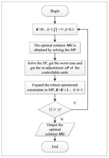
Figure 2.
The algorithm flow chart for model solving.
4. Simulation and Discussion
4.1. Simulation Information
The established model is verified on a CCHP micro-grid, which is shown in Figure 1. In order to show how the renewable energy (RE) affects the value of the EES in the CCHP microgrid, 4 cases are considered in the simulation. The results of the 4 cases are compared and analyzed in the following part. The specific settings of the 4 cases are as follows:
Case 1: Without RE and EES.
Case 2: Without RE and with EES.
Case 3: With RE and without EES.
Case 4: With RE and EES.
The uncertainty sets of WT and solar PV units generation are based on the wind speed and illumination data of typical days in each quarter. In the 4 cases, the Monte Carlo simulation method is used to generate light radiation scenarios, which is needed for building the uncertainty sets of solar PV units generation. The wind speed scenarios are generated with the Weibull probability density function. The time scale chosen in this paper is one day. The daily operation time is divided into 24 periods, where each period is an hour. The uncertainty sets of 24-h WT and solar PV units generation are shown in Figure 3 and Figure 4. The value of budgets and is 6. The forecast day-ahead price of power market is shown in Figure 5. The cooling, thermal and power load are shown in Figure 6. The other important parameters in the CCHP microgrid optimization model are shown in Table 1. This paper uses YALMIP solver toolbox of MATLAB (R2016a, MathWorks, Natick, MA, USA) to solve the model.
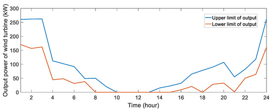
Figure 3.
Uncertainty range of output power of wind turbine.
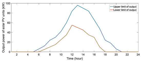
Figure 4.
Uncertainty range of output power of solar PV units.
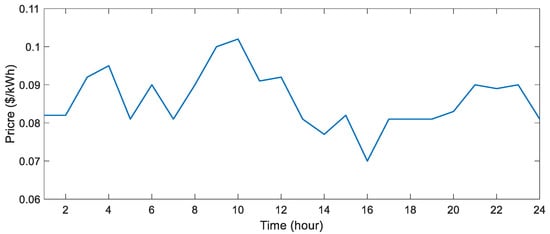
Figure 5.
Expected day-ahead market price curve.
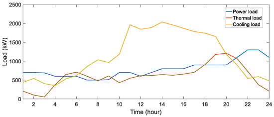
Figure 6.
The expected cooling, thermal and power load curve of the CCHP microgrid.

Table 1.
Simulation parameters.
4.2. Results and Discussion
The CCHP microgrid optimized operation cost in 4 cases is shown in Table 2. In Case 1, Case 2, Case 3, and Case 4, the CCHP microgrid optimized operation costs are $1518.03, $1391.11, $1419.68, and $1232.07, respectively. This results show that the renewable energy and the electrical energy storage will influence the CCHP microgrid scheduling and finally influence the operation cost. In order to simplify the analysis of this part, Case 1 and Case 2 are defined as Group 1; Case 3 and Case 4 are defined as Group 2. Economic analysis and sensitivity analysis of electrical energy storage will be discussed at the end of this section.
Table 2.
Optimal operation cost of the CCHP microgrid in 4 cases.
In Group 1, the CCHP microgrid operation cost without renewable energy is reduced by 8.36% after the CCHP microgrid installing the electrical energy storage. This shows that the CCHP microgrid can improve the flexibility of operation after installing the electrical energy storage. Due to the existence of the power price difference in electricity market, the CCHP microgrid can use the operation of EES to reduce the CCHP microgrid operation cost. In Group 2, the CCHP microgrid operation cost with renewable energy is reduced by 13.21% after the CCHP microgrid installing the electrical energy storage. Compared with Group 1 without renewable energy, the CCHP microgrid operation cost is reduced more after installing electrical energy storage. This shows that electrical energy storage in Case 4 can improve the stability of RE output and create more economic value.
The total CCHP microgrid operation cost and composition in four cases are shown in Figure 7. In the figure, positive value represents cost and negative value represents revenue. The sum of positive and negative values is the CCHP microgrid operation cost in this case. As shown in the figure, the cost of power energy transaction between the CCHP microgrid and MG accounts for the largest proportion of the total cost, followed by the cost of MT, the cost of GB and the environmental (ENV) cost. In Group 1, the environmental cost and the cost of MT and GB remained basically unchanged. The electrical energy storage can reduce the CCHP microgrid operation cost by reducing the purchase energy from MG and charging and discharging arbitrage. In Group 2, the environmental cost and the cost of GB remained basically unchanged. The electrical energy storage can reduce the reserved capacity of MT to deal with the volatility of RE generation and then reduce the CCHP microgrid operation cost by reducing the purchase of energy from MG and arbitrage. In Case 3 and Case 4, the abandoned power of wind turbine and solar PV unit is 0, which means the CCHP microgrid can promote renewable energy consumption.
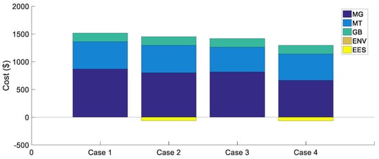
Figure 7.
The operation cost and composition of the CCHP microgrid under different cases.
After comparing the operation cost under four cases, the value of electrical energy storage can be calculated by analyzing the operation cost of the cases with and without electrical energy storage. For each group, the value of EES can be calculated as follows:
- EES value in Group 1 = Case 1 operation cost—Case 2 operation cost,
- EES value in Group 2 = Case 3 operation cost—Case 4 operation cost.
Figure 8 shows the EES comprehensive value and composition under the groups with the CCHP microgrid with and without renewable energy. As shown in the figure, the comprehensive value of energy storage is higher in Group 2 compared with Group 1. The electrical energy storage will also change MT operation state and then change MT operation cost. Figure 9 shows MT generation in four cases. Figure 10 shows the trading energy with the MG in four cases. In the figure, positive value presents the CCHP microgrid purchases energy from MG, and negative value presents the CCHP microgrid sells energy from MG. Figure 11 shows the EES output power in two cases. The positive value in the figure indicates the EES charging power and the negative value indicates the EES discharging power. As shown in the figure, MT output is basically the same under Case 1 and Case 2. From the results of this paper, in Group 1 without renewable energy, the electrical energy storage has no significant impact on the MT operation. In Group 2 with renewable energy, the electrical energy storage can reduce the reserve capacity provided by the MT for renewable energy and then increase MT output, which can cut the CCHP microgrid operation cost. It will increase the cost of MT and environmental cost while reducing the cost of power energy purchase. As shown in Figure 10 and Figure 11, compared with Case 3, the input power of the main grid is lower and the time of output power of the main grid is more frequent in Case 4. At the same time, for the sake of reducing the volatility of RE output, the electrical energy storage needs to reserve part of the capacity. Therefore, the operation of EES is less active in Case 4.
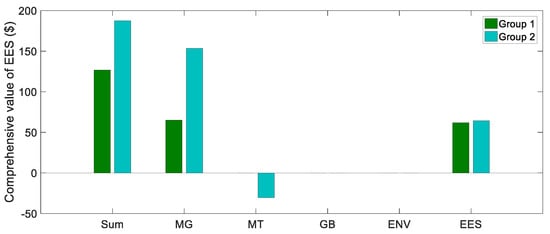
Figure 8.
Comprehensive value and composition of the EES under 2 Groups.
Figure 9.
MT output power under 4 Cases.
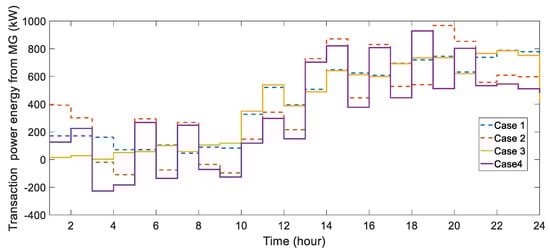
Figure 10.
The transaction power energy from the MG under 4 Cases.
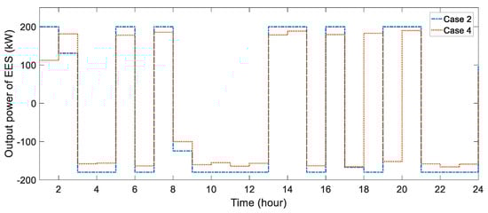
Figure 11.
The output power of the EES under 2 Cases.
The economic analysis of net present value (NPV) of the EES power plant is carried out in this paper. NPV refers to the sum of the net cash flow discounted to the present value at the beginning of the project according to a certain discount rate. The calculation and analysis of the investment benefit of energy storage plant is based on the cash inflow and cash outflow in each year of the life cycle, which correspond to the operation income and operation cost of each year in the life cycle, respectively. The calculation formula is as follows:
where is the net cash flow in year ; accounts for cash inflow, that is, the annual revenue of EES; presents cash outflow; and n are discount rate and life cycle of the EES power station; and indicate the total investment cost and operation and maintenance cost in the year ; is cash flow factor; and demonstrate the unit power conversion system capital expenditure and unit storage capital expenditure respectively; D is the total operation days of the EES power plant in a year. and account for the discharging and charging power of the EES at the time of the day .
In the calculation of this paper, the EES power plant installed in the CCHP is lithium ferrophosphate batteries with mature technology and common application. The parameter values are as follows: -$300/kW, -$228/kWh, -7%, n-8, and the residual value rate of the EES power plant is 5% after the end of the operation life. Three cases are constructed for NPV calculation. In Case 1, the EES power plant can only obtain arbitrage revenue (AR) brought by charging and discharging power to help renewable energy consumption. In Case 2, the revenue of the EES equals its comprehensive value (CV). In Case 3, on the basis of the Case 2, the EES can reduce the CO2 emission of the CCHP microgrid and it is assumed that the CCHP microgrid can participate in the carbon market. Carbon price is based on the Regional Greenhouse Gas Initiative (RGGI) carbon market in September 2019, which is $5.20/t.
The results are shown in Figure 12. In Case 1, if the EES can only obtain arbitrage revenue, the NPV is −87.82 thousand dollars. This shows that in this scenario, it is not attractive for investors to build an energy storage power plant, for its revenues cannot cover costs and the net revenue is negative. In Case 2 and Case 3, the NPV of the EES power plant is 180.61 and 269.26 thousand dollars, respectively. This shows that the comprehensive value of EES to the CCHP system can make the project owner obtain revenues. With the development of carbon market, the value of EES will further increase. In this particular example, though comprehensive value over the costs, the available profit is less than the costs, making the project economically infeasible for the investors. It is beneficial for the whole system to put the EES power plant into operation. System managers need to understand the comprehensive value of EES so as to support cost-effective storage deployment.
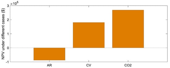
Figure 12.
The NPV of the EES under 3 Cases.
Sensitivity analysis of the RE penetration, market price difference coefficient (PDC), total capital expenditure, and the capacity of EES are also carried out in this paper. The PDC represents the degree of electricity price fluctuation which is calculated as follow:
where is PDC; presents the electricity price higher than the average price; indicates the electricity price is the electricity price below average price; is the average price.
Figure 13 shows the sensitivity analysis results of RE penetration level and PDC. It can be seen that with the increase of RE penetration rate and PDC, the NPV of EES is also increasing. This shows that EES can achieve better performance and obtain more value in the scenario of high RE penetration and large price fluctuation. Through the comparison of curves position and slope, it can be seen that the influence of RE penetration on EES revenue is greater than that of PDC. Under the same degree of change, the rise of the RE penetration level will bring more value and bring more marginal value as well. This shows that in the future, with the continuous development of RE and the continuous rising of the RE penetration level, EES will perform better and obtain more value.
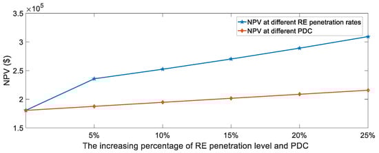
Figure 13.
Sensitivity analysis of RE penetration level and market price difference coefficient (PDC).
Figure 14 shows the sensitivity analysis results of EES capacity and total capital expenditure. In the figure, the blue line indicates the influence on increased EES capacity on NPV of EES, and the red line indicates the influence on the reduction of total capital expenditure on NPV of EES. It is thus clear that the growth of EES capacity has little effect on NPV. With the increase of EES capacity, NPV first increases and then decreases. This shows that there is a reasonable interval for the allocation of EES capacity. If it exceeds the reasonable range, the marginal revenue from the increased capacity is not enough to make up for the marginal capital cost brought by the increase of capacity, so the benefit of EES will decrease. With the decrease of total capital expenditure, the NPV of EES increases gradually. This shows that with the continuous development of EES technology, the cost of EES gradually decreases, and the comprehensive value of EES will further increase.
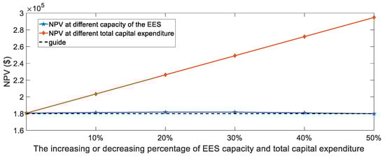
Figure 14.
Sensitivity analysis of EES capacity and total capital expenditure.
5. Conclusions
In this article, a robust optimization model of the CCHP microgrid participating in power market transaction is constructed to calculate the CCHP microgrid operation cost in 4 cases. The results show that EES can significantly cut the CCHP microgrid cost by 13.21%, compared with 8.36% in Group 1 without renewable energy. The electrical energy storage can reduce the reserved capacity of MT to deal with the volatility of RE generation and then reduce the CCHP microgrid operation cost by reducing the purchase of energy from MG and arbitrage. Finally, the calculation method of EES comprehensive value is constructed. The comprehensive value of EES includes the cost reduction of the MT, environment, and power energy transaction from MG and arbitrage. The comprehensive value of electrical energy storage is higher in Group 2 with renewable energy compared with Group 1 without renewable energy. Through NPV calculation and sensitivity analysis, it is found that the RE penetration level and EES cost have the greatest impact on the economic performance of EES. This shows that with the continuous improvement of the RE penetration level and the gradual decrease of EES cost, great potential still waits to be tapped in the comprehensive value of EES in the future.
In the last few years, with the practice and popularization of the demand response program, this research can be extended to discuss EES value applying in the demand response program. The EES can be applied to cooling thermal and power demand to measure the EES value applying in the CCHP microgrid demand response program.
Author Contributions
H.L. proposed the concept of this research and completed the manuscript. X.W., B.L. and P.L. analyzed the empirical data. H.Z., Y.W. and Z.M. gave some suggestions. All authors have read and agreed to the published version of the manuscript.
Funding
This research received no external funding.
Acknowledgments
This study is supported by the National Natural Science Foundation of China (Grant No.71973043), the Fundamental Research Funds for the Central Universities (2019QN077), and the Natural Science Foundation of Hebei Province of China (G2020502004).
Conflicts of Interest
The authors declare no conflict of interest.
Appendix A
The second stage:
- (1)
- Constraints for multiple power balances:
- (2)
- Operational constraints for MT
- (3)
- Operational constraints for EES:
- (4)
- Operational constraints for the GB, HR, EC, AC and the main grid:
References
- Pu, L.; Wang, X.; Tan, Z.; Wang, H.; Yang, J.; Wu, J. Is China’s electricity price cross-subsidy policy reasonable? Comparative analysis of eastern, central, and western regions. Energy Policy 2020, 138, 111250. [Google Scholar] [CrossRef]
- Lin, B.; Ankrah, I. Renewable energy (electricity) development in Ghana: Observations, concerns, substitution possibilities, and implications for the economy. J. Clean. Prod. 2019, 233, 1396–1409. [Google Scholar] [CrossRef]
- McGee, J.; Greiner, P.T. Renewable energy injustice: The socio-environmental implications of renewable energy consumption. Energy Res. Soc. Sci. 2019, 56, 101214. [Google Scholar] [CrossRef]
- Obara, S.; Sato, K.; Utsugi, Y. Study on the operation optimization of an isolated island microgrid with renewable energy layout planning. Energy 2018, 161, 1211–1225. [Google Scholar] [CrossRef]
- Ajeigbe, O.A.; Munda, J.; Hamam, Y. Optimal Allocation of Renewable Energy Hybrid Distributed Generations for Small-Signal Stability Enhancement. Energies 2019, 12, 4777. [Google Scholar] [CrossRef]
- Heitkoetter, W.; Medjroubi, W.; Vogt, T.M.; Agert, C. Comparison of Open Source Power Grid Models—Combining a Mathematical, Visual and Electrical Analysis in an Open Source Tool. Energies 2019, 12, 4728. [Google Scholar] [CrossRef]
- Davison-Kernan, R.; Liu, X.; McLoone, S.; Fox, B. Quantification of wind curtailment on a medium-sized power system and mitigation using municipal water pumping load. Renew. Sustain. Energy Rev. 2019, 112, 499–507. [Google Scholar] [CrossRef]
- Wang, Q.; Zhan, L. Assessing the sustainability of renewable energy: An empirical analysis of selected 18 European countries. Sci. Total Environ. 2019, 692, 529–545. [Google Scholar] [CrossRef]
- Zhao, H.; Li, B.; Wang, X.; Lu, H.; Li, H. Evaluating the performance of China’s coal-fired power plants considering the coal depletion cost: A system dynamic analysis. J. Clean. Prod. 2020, 275, 122809. [Google Scholar] [CrossRef]
- Hussain, A.; Bui, V.-H.; Bui, V.-H.; Im, Y.-H.; Lee, J.Y. Optimal Energy Management of Combined Cooling, Heat and Power in Different Demand Type Buildings Considering Seasonal Demand Variations. Energies 2017, 10, 789. [Google Scholar] [CrossRef]
- Woo, C.K.; Zarnikau, J. Renewable energy’s vanishing premium in Texas’s retail electricity pricing plans. Energy Policy 2019, 132, 764–770. [Google Scholar] [CrossRef]
- Yao, S.; Zhang, S.; Zhang, X. Renewable energy, carbon emission and economic growth: A revised environmental Kuznets Curve perspective. J. Clean. Prod. 2019, 235, 1338–1352. [Google Scholar] [CrossRef]
- Gharibeh, H.F.; Yazdankhah, A.S.; Azizian, M.R. Energy management of fuel cell electric vehicles based on working condition identification of energy storage systems, vehicle driving performance, and dynamic power factor. J. Energy Storage 2020, 31, 101760. [Google Scholar] [CrossRef]
- Hou, H.; Xu, T.; Wu, X.; Wang, H.; Tang, A.; Chen, Y. Optimal capacity configuration of the wind-photovoltaic-storage hybrid power system based on gravity energy storage system. Appl. Energy 2020, 271, 115052. [Google Scholar] [CrossRef]
- Balsamo, F.; Capasso, C.; Lauria, D.; Veneri, O. Optimal design and energy management of hybrid storage systems for marine propulsion applications. Appl. Energy 2020, 278, 115629. [Google Scholar] [CrossRef]
- Hao, Y.; He, Q.; Du, D. A trans-critical carbon dioxide energy storage system with heat pump to recover stored heat of compression. Renew. Energy 2020, 152, 1099–1108. [Google Scholar] [CrossRef]
- Zhao, H.; Guo, S.; Zhao, H. Comprehensive assessment for battery energy storage systems based on fuzzy-MCDM considering risk preferences. Energy 2019, 168, 450–461. [Google Scholar] [CrossRef]
- Yazdani, S.; Deymi-Dashtebayaz, M.; Salimipour, E. Comprehensive comparison on the ecological performance and environmental sustainability of three energy storage systems employed for a wind farm by using an emergy analysis. Energy Convers. Manag. 2019, 191, 1–11. [Google Scholar] [CrossRef]
- Han, X.; Wei, Z.; Hong, Z.; Liang, D. Adaptability assessment method of energy storage working conditions based on cloud decision fusion under scenarios of peak shaving and frequency regulation. J. Energy Storage 2020, 32, 101784. [Google Scholar] [CrossRef]
- Rodrigues, D.L.; Ye, X.; Xia, X.; Zhu, B. Battery energy storage sizing optimisation for different ownership structures in a peer-to-peer energy sharing community. Appl. Energy 2020, 262, 114498. [Google Scholar] [CrossRef]
- Afzali, P.; Shoa, N.A.; Rashidinejad, M.; Bakhshai, A. Techno-economic study driven based on available efficiency index for optimal operation of a smart grid in the presence of energy storage system. J. Energy Storage 2020, 32, 101853. [Google Scholar] [CrossRef]
- Mostafa, M.H.; Aleem, S.H.E.A.; Ali, S.G.; Ali, Z.M.; Abdelaziz, A.Y. Techno-economic assessment of energy storage systems using annualized life cycle cost of storage (LCCOS) and levelized cost of energy (LCOE) metrics. J. Energy Storage 2020, 29, 101345. [Google Scholar] [CrossRef]
- Liu, J.; Hu, C.; Kimber, A.; Wang, Z. Uses, Cost-Benefit Analysis, and Markets of Energy Storage Systems for Electric Grid Applications. J. Energy Storage 2020, 32, 101731. [Google Scholar] [CrossRef]
- Khastieva, D.; Hesamzadeh, M.R.; Vogelsang, I.; Rosellon, J.; Amelin, M. Value of energy storage for transmission investments. Energy Strat. Rev. 2019, 24, 94–110. [Google Scholar] [CrossRef]
- Sharma, P.; Kolhe, M.; Sharma, A. Economic performance assessment of building integrated photovoltaic system with battery energy storage under grid constraints. Renew. Energy 2020, 145, 1901–1909. [Google Scholar] [CrossRef]
- Ogland-Hand, J.D.; Bielicki, J.M.; Wang, Y.; Adams, B.M.; Buscheck, T.A.; Saar, M.O. The value of bulk energy storage for reducing CO2 emissions and water requirements from regional electricity systems. Energy Convers. Manag. 2019, 181, 674–685. [Google Scholar] [CrossRef]
- Zhao, H.; Lu, H.; Li, B.; Wang, X.; Zhang, S.; Wang, Y. Stochastic Optimization of Microgrid Participating Day-Ahead Market Operation Strategy with Consideration of Energy Storage System and Demand Response. Energies 2020, 13, 1255. [Google Scholar] [CrossRef]
- Wang, Y.; Tang, L.; Yang, Y.; Sun, W.; Zhao, H. A stochastic-robust coordinated optimization model for CCHP micro-grid considering multi-energy operation and power trading with electricity markets under uncertainties. Energy 2020, 198, 117273. [Google Scholar] [CrossRef]
- Wang, Y.; Yang, Y.; Tang, L.; Sun, W.; Li, B. A Wasserstein based two-stage distributionally robust optimization model for optimal operation of CCHP micro-grid under uncertainties. Int. J. Electr. Power Energy Syst. 2020, 119, 105941. [Google Scholar] [CrossRef]
- Cui, Q.; Ma, P.; Huang, L.; Shu, J.; Luv, J.; Lu, L. Effect of device models on the multiobjective optimal operation of CCHP microgrids considering shiftable loads. Appl. Energy 2020, 275, 115369. [Google Scholar] [CrossRef]
- Kim, H.; Kim, M.-K.; Lee, J. A two-stage stochastic p-robust optimal energy trading management in microgrid operation considering uncertainty with hybrid demand response. Int. J. Electr. Power Energy Syst. 2021, 124, 106422. [Google Scholar] [CrossRef]
- Ji, L.; Niu, D.; Huang, G. An inexact two-stage stochastic robust programming for residential micro-grid management-based on random demand. Energy 2014, 67, 186–199. [Google Scholar] [CrossRef]
- Zhu, C.; Xu, B.; Nie, Y.Z. An Integrated Design and Operation Optimal Method for CCHP System. Energy Procedia 2019, 158, 1360–1365. [Google Scholar] [CrossRef]
- Guo, J.; Li, Y.; Shen, Y.; Li, H. An incentive mechanism design using CCHP-based microgrids for wind power accommodation considering contribution rate. Electr. Power Syst. Res. 2020, 187, 106434. [Google Scholar] [CrossRef]
- Cao, Y.; Wang, Q.; Du, J.; Nojavan, S.; Jermsittiparsert, K.; Ghadimi, N. Optimal operation of CCHP and renewable generation-based energy hub considering environmental perspective: An epsilon constraint and fuzzy methods. Sustain. Energy, Grids Netw. 2019, 20, 100274. [Google Scholar] [CrossRef]
- Qasemi, K.; Azadani, L.N. Optimization of the power output of a vertical axis wind turbine augmented with a flat plate deflector. Energy 2020, 202, 117745. [Google Scholar] [CrossRef]
- Zaraket, J.; Aillerie, M.; Salame, C.; Losson, E. Output Voltage Changes in PV Solar Modules after Electrical and Thermal Stresses. Experimental Analysis. Energy Procedia 2019, 157, 1404–1411. [Google Scholar] [CrossRef]
- Jalali, M.; Zare, K.; Seyedi, H.; Alipour, M.; Wang, F. Distributed model for robust real-time operation of distribution systems and microgrids. Electr. Power Syst. Res. 2019, 177, 105985. [Google Scholar] [CrossRef]


Publisher’s Note: MDPI stays neutral with regard to jurisdictional claims in published maps and institutional affiliations |
© 2020 by the authors. Licensee MDPI, Basel, Switzerland. This article is an open access article distributed under the terms and conditions of the Creative Commons Attribution (CC BY) license (http://creativecommons.org/licenses/by/4.0/).