Abstract
This paper proposes a particle filter (PF)-based electricity load prediction method to improve the accuracy of the microgrid day-ahead scheduling. While most of the existing prediction methods assume electricity loads follow normal distributions, we consider it is a nonlinear and non-Gaussian process which is closer to the reality. To handle the nonlinear and non-Gaussian characteristics of electricity load profile, the PF-based method is implemented to improve the prediction accuracy. These load predictions are used to provide the microgrid day-ahead scheduling. The impact of load prediction error on the scheduling decision is analyzed based on actual data. Comparison results on a distribution system show that the estimation precision of electricity load based on the PF method is the highest among several conventional intelligent methods such as the Elman neural network (ENN) and support vector machine (SVM). Furthermore, the impact of the different parameter settings are analyzed for the proposed PF based load prediction. The management efficiency of microgrid is significantly improved by using the PF method.
1. Introduction
Since the increasing penetration level of renewable-based distributed generators (RE-DGs) such as photovoltaic-based (PV) arrays and wind turbines [1], the energy management and operation of a microgrid becomes more challenging. The uncertainty introduced by these RE-DGs and electricity loads emphasizes the importance of an accurate prediction method in the microgrid day-ahead scheduling [2,3]. The neural network method is a typical representative of data-driven forecasting methods. It is widely used in the predicting electricity load [4,5,6]. A variety of new neural network structures are produced by combining with other techniques in forecasting research, such as Elman neural network (ENN) [7,8,9], recurrent neural networks (RNN) [10,11,12,13], recurrent extreme learning machine (RELM) [14]. These new neural networks not only have the structural advantages of traditional neural networks, but also have some improvements in calculation efficiency and operating cost. Besides, some mature artificial intelligence algorithm models (such as support vector machines (SVM) [15,16,17,18], support vector regression (SVR) [19,20], and fuzzy logic [21,22]) that used to solve prediction problems with nonlinear characteristics, are applied to forecast electricity load. Due to the difference of the practical problems and the diversity of feature selection methods, there is no regular feature selection model method and various classifiers have different effects on the result of feature selection. It is difficult to determine which feature selection method can bring optimal estimated performance to the model for the first time when facing practical problems. Another important factor affecting data-driven method is data sampling.
In practice, the data provided to the power load system is affected by the operative mode of the equipment, and the operating environment, which are regularly non-linear and non-Gaussian as shown in Figure 1. It can not accurately predict for traditional intelligent forecasting models. To get more accurate prediction results, A hybrid model based on improved empirical mode decomposition, autoregressive integrated moving average, and wavelet neural network optimized by fruit fly optimization algorithm is presented by Zhang et al. [23]. The hybrid model divided the state information of power load into two parts: linear and nonlinear. The linear part is regarded as a definite linear time series, which changes steadily with time. The nonlinear part has high volatility and randomness, which is mainly affected by historical power load and future weather conditions (such as temperature). However, this disadvantage is to increase the calculation cost and accumulated error caused by the separate calculation. For addressing the issues in data-driven, the particle filter (PF) method is introduced to electricity load forecasting, and optimal assign power references to make better decisions in microgrid day-ahead scheduling. According to the literatures, PF-based method has been widely used in remaining useful life forecasting [24,25,26,27], filtering and state estimation for nonlinear systems [28,29,30]. Since the particle filter is on the basis of Bayesian sampling estimation, it is better suitable for solving nonlinear and non-Gaussian problem. As a sequential important sampling (SIS) filter algorithm, the probability density function (PDF) of the particle filter is represented by particles. The PDF will change with particles. Therefore, the prediction precision of the PF-based method is higher than the traditional function-driven method for electricity power load. To our knowledge, this is the first description in the literature of the using PF-based method for electricity load forecasting in day-ahead scheduling.
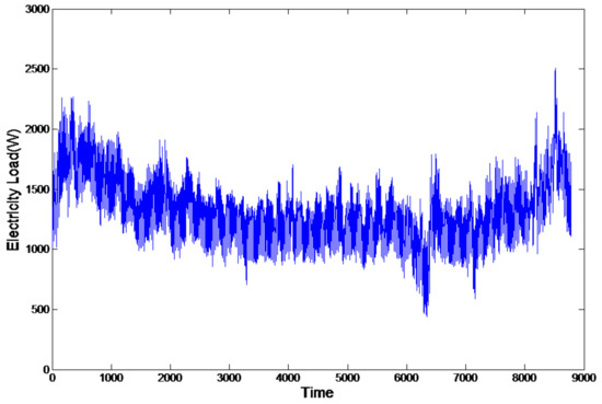
Figure 1.
Variations of actual electricity load of in the city of Ottawa during the year 2004.
Our work and innovation are emphasized in the rest of this paper which is organized as follows: Section 2 provides deterministic grid-connected microgrid day-ahead scheduling formulation is built. Section 3 is the description of the PF method. Comparison results on a distribution system with ENN-based method and SVM-based method are shown in Section 4. The analysis results of Day-ahead scheduling are also presented in this section. The influence factors and the number of particles for the PF method are discussed in Section 5. The final section concludes the paper.
2. Deterministic Grid-Connected Microgrid Day-Ahead Scheduling Formulation
As the same as most previous studies, the deterministic grid-connected microgrid day-ahead scheduling can be regarded as the nonlinear optimization problem Equation (1) [31]:
All parameters and corresponding notations are shown in Table 1.

Table 1.
Nomenclature, reprint with permission [31], 2017, IET GTD.
For this microgrid day-ahead scheduling, the main objective is to obtain optimized cost by rationalizing the distribution which utilizes forecasted power production from uncontrollable DGs and loads demand of power references for all controllable DGs. It can be seen from the cost function as shown in Equation (1), the is an active power. It means that the can be either positive or negative. When is positive, it needs to be injected from the main grid. Because the power produced by the DGs is less than the consumed power by load. On the contrary, when is negative, the power produced by the DGs is more than the consumed power by load, it can be transported to the main grid. As shown in Figure 2, the photovoltaic prediction data, the time of use (TOU) electricity price, and all-day prediction load data are the main input parameters for day-ahead optimal scheduling. Since the TOU is fixed, the PV is relatively stable and less fluctuation, the accuracy of OPF is mainly determined by the precision of the electricity power load prediction. Hence, it is imperative to accurately predict electricity power load demand. Since the variation of actual electricity load is drastic and non-Gaussian distribution, it is a huge challenge to predict electricity load by using the general prediction method. Moreover, OPF is not a linear system model due to it consisting of various kinds of noise distributions. Although we use the Modified Harr two-point model to estimate the variation ranges, it cannot accurately predict the electricity load. The estimation accuracy and efficiency of this method are easily infected by the number of input variables. In the past, the traditional Kalman filter (KF) was extensively used to load forecasts. However, the deficiency of KF-based method is that it is not suitable for the non-Gaussian and nonlinear system dynamics of electricity load. Furthermore, the calculation burden of the KF-based method is too heavy. Since the particle filter is on the basis of Bayesian sampling estimation, it is better suitable for solving nonlinear and non-Gaussian problem. As a sequential important sampling (SIS) filter algorithm, the probability density function (PDF) of the particle filter is represented by particles. The PDF will change with particles. Hence, satisfactory prediction results were achieved by utilizing PF-based method for electricity power load in grid-connected microgrid day-ahead scheduling.
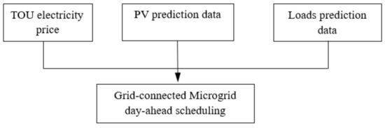
Figure 2.
Key input for grid-connected mircrogrid day-ahead scheduling.
3. Particle Filtering Based Prediction
As mentioned above, the actual electricity load system is nonlinear and non-Gaussian, so it is unsuitable to analyze the electricity load forecasting problem using analytic methods. Particle Filter which also called Bayesian Importance Sampling relies upon a sequential important sampling (SIS) filter algorithm. For nonlinear and non-Gaussian systems, it is often complicated to get an analytic solution. In order to avoid the problem, the integration is used to investigate the solution of nonlinear operator equation in the PF-based method. Furthermore, the integral calculations are substituted by a series of particles. According to their importance, the particles will be given different weights in the posterior probability density. The error between the distribution characteristics represented by particles and the posterior probability distribution of the system state gradually decreases as the number of particles increased. When the particles reached a certain scale, it is approximately equal to each other. The represents active power demand. In the paper, it can be estimated by the probability density function which is constructed from measured active power. The details are as follows:
The t and represent time step and sampling interval, respectively. The is the required power in the starting stage. According to iteration criteria, the value of can be calculated the . In addition, the represents the measured value by sensor. The represents degradation or increasing rate, C represents discrete change with unusual demand active power. , C follow the complex Gaussian distribution with , . The is random noise at time step t.
Similar to other SIS algorithms, the posterior PDF can be represented by a set of random particles with their associated weights as follows:
where i is the i-th particle, N is the number of particles. The weights for each particles is variable and constantly updating. It is determined by the observed values of the system. For each particle,
where, is the observed value, is the unobserved system state, is the transition density function. and the is the optimal function. Since it is complicated to establish a suitable optimization function, it is common to select
The modified algorithm flow is described as shown in Figure 3.
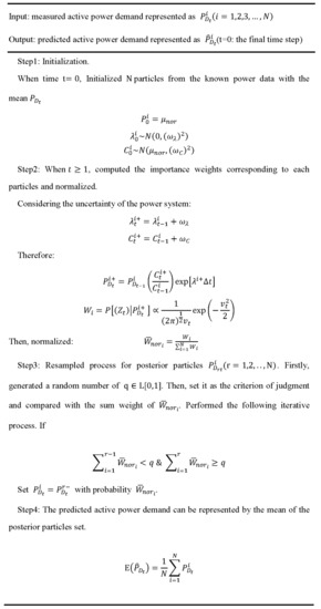
Figure 3.
The development PF-based algorithm flow.
4. Case Studies and Validations
To prove the effectiveness of the PF-based algorithm, an equivalent 44 kV distribution feeder system in the city of Ottawa (see Figure 4) is used to test load prediction for distribution system day-ahead scheduling. It can be seen from Figure 4, this system contains a 230 kV utility source, a 230/44 kV transformer, a 20 Mvar capacitor bank, two circuit breakers, a PV-DGs, a natural gas turbine and a diesel generator. There are six loads in the system. Readers can refer our previous paper [31] for detailed system parameters. According to [32], the PV power is calculated by solar irradiance, system load data and temperature. In this work, for the simplification, we assume that the measurements of solar irradiance and temperature are consistent with the actual value. Therefore, the accuracy of the distribution system day-ahead scheduling is only affected by the prediction accuracy of the system load. In the rest of this section, we will analyze the electricity load prediction based on the PF method. Then, the impact of load forecast errors on the microgrid day-ahead scheduling is investigated. Furthermore, we compare our proposed particle filter method with two typical artificial intelligence methods including SVM and ENN.
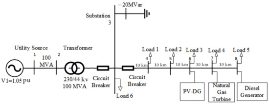
Figure 4.
Equivalent distribution feeder system.
4.1. Electricity Load Prediction
The historical electricity load data of Ottawa, for two years (from 1 January 2004, 24:00 to 31 December 2005, 24:00) is utilized to confirm the accuracy and validity of our presented PF-based method. Furthermore, to validate the effectiveness and performance of PF-based method, we compare our proposed method with two maturely and commonly used electricity load intelligent predicting methods, i.e., SVM and ENN.
Firstly, the electricity load data set was divided into two categories. The data from 1 January 2004 to 31 December 2004 composed the training set. The rest of the data from 1 January 2005 to 31 December 2005 was composed the set. For the sake of narrative and to make the results clear, we selected three typical moments of every day (i.e., 10:00, 15:00, and 21:00) for discussion. The year divide into spring (January, February, March), summer (April, May, June), autumn (July, August, September) and winter (October, November, December) seasons in 2004 and 2005. This representation provides the expected results for the whole year.
The predicted results for electricity load in different moments are shown in Figure 5. The errors between predictions and actual values are also shown in these figures. It can be seen from Figure 5, comparing with SVM and ENN, the PF-based method predictions (represented in red star) is the most accurate. Furthermore, it can accurately represent the trend of the actual measured value (represented in black circle) by the sensor. Especially in the summer and winter, even when the electricity load vary more dramatically than other seasons, the PF-based method is more efficient and stable predictions than SVM and ENN. Note that the vertical bold black lines in the picture are the border lines of different data sets (training and testing, respectively). It is not difficult to find that the trend of electricity load in the two years is roughly the same.
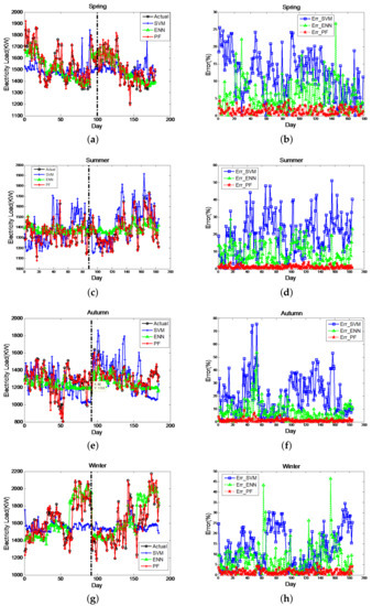
Figure 5.
Four seasons of electricity load predictions and errors at 10:00 everyday. (a) predictions of Spring, (b) errors of Spring, (c) predictions of Summer, (d) errors of Summer, (e) predictions of Autumn, (f) errors of Autumn, (g) predictions of Winter, (h) errors of Winter.
As for the moment of 10:00 in the morning, Figure 5 shows the comparisons of the different predicting method and actual electricity load. It is obvious that PF-based method is relatively better with an error less than 5% while the SVM-based and ENN-based are almost more than 10% and 20%, respectively. Hence, the prediction accuracy of electricity load was improved by around 50% by using our proposed PF-based method. Furthermore, the biggest error of SVM-based in autumn reached 75.6%. The worst predicted result in winter of ENN-based is 46.2%. However, the results of PF-based for four seasons are stable except for a few unusual results in the fall. Since the figure shows similar results for the moment of 15:00 in the afternoon and 21:00 in the evening, we do not give these figures in this paper. Comparing with SVM-based and ENN-based methods, the PF-based method achieved higher precision at the moment of 15:00 in the afternoon. The predicted curve almost coincides with the actual electricity load. The forecast error is less than 10% in spring and summer. The most of error in winter is below 5%. The mean absolute percentage error (MAPE) of the PF-based method is about 3%. There are also some poor predictions which are up to about 20% as the same as mentioned before. For the moment of 21:00 in the evening, all of these three method have relatively poor predicting behaviors. For the SVM-based and ENN-based methods, most errors are in the range of 10–30% in spring, summer and winter. In the fall, the performance of the SVM-based method is poor. The biggest error of this method is about 67.2%. Although the PF-based method also has some unusual results in four seasons, most of the results are satisfactory. Especially the largest error rate in fall of PF-based method is 17.6% which is also the biggest error in all seasons and all moments mentioned before. Therefore, we can come to the conclusion that the PF-based method is predicted to be more accurate than the other two methods.
Furthermore, due to the MAPE and standard deviation (SD) are easy to understand, the MAPE and (SD) is used to represent the accuracy of different algorithm. The detailed mathematical definition for MAPE and (SD) are as follows:
where is the actual measured value of electricity load for kth day, is the prediction of electricity load for kth day, N is the number of days predicted, is the mean of actual electricity load. The performance indicators of SVM, ENN, and PF are given in Table 2.
Table 2.
Performance metrics of different algorithms for electricity load prediction.
As shown in Table 2, all performance indicators of our proposed PF-based method are lower than ENN-based and SVM-based algorithms for four seasons at different moments. It is clear that the PF-based method is more accurate than the other two comparison methods. Specifically, the fluctuation range of MAPE values based on PF-based method is 1.01–3%. The SVM-based and ENN-based fluctuation ranges are 7.04–13.24%, 4.47–9.33%, respectively. The maxima and minima of MAE for PF-based method is 41.55 and 9.54. The maximum and minimum values for the other two methods are 171.47 and 68.03, which are several higher than the PF-based algorithm. For the performance metrics of RMSE, the PF-based method is in the range of 0.95–3.35. However, the SVM-based method and ENN-based method are in the range of 10.06–16.04, 6.38–13.91, respectively. Therefore, obviously, the prediction accuracy of the PF-based method is higher and more stable than SVM-based and ENN-based for electricity load predicted.
4.2. Impact of Prediction Errors on Microgrid Day-Ahead Scheduling
As mentioned in Section 2, the microgrid day-ahead scheduling is used to optimize operation through accurately predicting power production from uncontrollable DGs and load demand to reasonably allocate the optimal reference power to all controllable DGs. This means when the load demand predictions have higher accuracy, then the reference power will be more suitable. So it can achieve optimal operation by reducing cost. After comparing and verifying the accuracy and stability of the PF-based method for electricity load which is utilized to discuss the scheduled DGs . Similarly, we also compared the three different methods at 10:00, 15:00 and 21:00 for four seasons. The comparing results are presented in Figure 6, Figure 7 and Figure 8. It is confirmed that the forecasted power by PF-based method fits active power more accurately than the other two methods at every moment in four seasons. Moreover, the PF-based method performs with better stability than SVM-based and ENN-based method for forecasting. The summary of calculating results of the scheduled DG power is presented in Table 3.
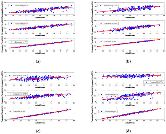
Figure 6.
The regression results of active power for four seasons at 10:00 every day, (a) spring, (b) summer, (c) autumn, (d) winter.
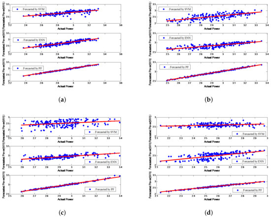
Figure 7.
The regression line of active power for four seasons at 15:00 every day, (a) spring, (b) summer, (c) autumn, (d) winter.
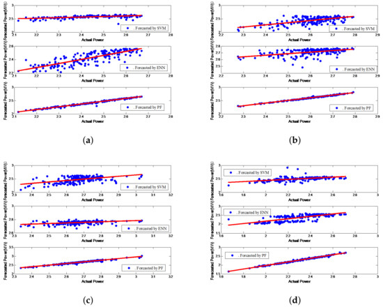
Figure 8.
The regression line of active power for four seasons at 21:00 every day, (a) spring, (b) summer, (c) autumn, (d) winter.
Table 3.
Impaction of predicted errors on microgrid day-ahead scheduling for different algorithms.
As seen from Figure 6, the regression estimates for forecasting power using a different method at each active (actual) power along the regression line shown in these figures. The forecasting power by PF-based method was performed with actual power in every season at 10:00. It is obvious that the MAPE values of all seasons are not more than 1%. However, the MAPE values of ENN-based method and SVM-based method are both higher than 2%. The maximum error occurs at utlizing the SVM-based method whose MAPE value is 7.97 in the summer. Furthermore, it is not difficult to see that our proposed PF-based algorithm obtained more stable forecasting than others. Especially, the MAPE value of summer (0.41) is approximately equal to the value of autumn (0.42) for the PF-based method.
For the moment of 15:00 and 21:00, Figure 7 and Figure 8 show the obtained regression lines of the comparison for the different methods. The results also demonstrate the superiority of the PF-based method. Specifically, all the MAPE values of our proposed PF-based algorithm is less than 1.5%. The maximum and minimum are 1.36% and 0.33%, respectively. The MAPE values of the other two methods are quite different. The maximum and minimum are 8.48% and 2.80%, respectively. It means that the PF-based method achieved nearly 7–8 times less MAPE than the other method. Therefore, this superiority is especially clear when comparing with the ENN-based and SVM-based method.
Additionally, as shown in Table 2 and Table 3, it is noticed that all evaluation criterion of the PF-based method for electricity load is better than SVM-based method and ENN-based method. Same as electricity load, the calculating results of scheduled DG power for PF-based method outperforms the other two methods. The reason is that prediction errors are inherently unavoidable. Since the PF-based method has better forecasting performance, is stable for all the testing electricity load data, the calculating results of scheduled DG power is also better beyond doubt.
5. Discussion
The testing results and comparisons confirmed that our proposed PF-based algorithm is powerful and stable for forecasting electricity load. Furthermore, due to more accurate predictions of electricity load, it will assign optimal power references active power for all controllable DGs, and make better operational decisions for microgrid day-ahead scheduling. This means that the management of microgrid day-ahead scheduling is greatly determined by the accuracy of the electricity load prediction.
Since the setting of relevant parameters of the particle filter algorithm is important to the accuracy of predictions, it is not trivial to find the optimal parameters. Firstly, the quantity of selected particles will have a direct impact on calculating time in the prediction process, large amounts of particles will lead to temporal redundancy in the computation, or the accuracy of the forecast is decreased. Next, the setting of system noise is also extremely important to the accuracy of the predicted result. The forecast data will have little variation when the system noise is too small. Otherwise, it will make the data change too violent and lead the forecasting data to deviate from the actual value. The selection of different parameter values for the particle filter algorithm on the prediction result has distinct effects, as shown in Figure 9. The comparison results of the particle filter algorithm within different parameters are carried out. Results obtained are shown in Table 4, where it can be clearly observed that the accuracy of the forecast results decreased significantly when the parameter is not getting properly selected. When the parameters of the PF algorithm are select to be sub-optimal, the accuracy of prediction results is still higher than other algorithms, but it is not the highest. It notes that improper parameters (for instance, particle leanness and strong noise) will result in higher prediction errors. The best prediction results came from only when the parameters are optimal. As for solving different practical problems, there is no fixed criterion for the selection of calculation parameters in the particle filter. Therefore, the process of particle filter optimal prediction becomes complicated. The setting of the number of particles in the particle filter algorithm will directly affect the computing time of the prediction process and the accuracy of the prediction results. Generally speaking, the more particles you set, the more accurate the prediction result will be. The computing time will increase accordingly. In order to reduce the computational cost under the premise of ensuring a certain prediction accuracy, we conduct preliminary comparison experiments to select the optimal number of particles. Through the comparative experiment of setting different particle numbers in three typical time periods in the spring of 2004 as shown in Table 5. It can be seen from the prediction results that when the number of particles is between 100 and 2500 and the number of set particles increases, the MAPE of the prediction results will gradually decrease while the computing time will gradually increase. When the number of particles set is increased to 3000, the computing time is still increasing, but the accuracy of the prediction results has no obvious change at this time. Compared with the setting of 2500 particles, the MAPE of the prediction results is only reduced by 0.1%. Therefore, in the actual prediction process of the particle filter, the optimal number of particles is set to 2500, so that the prediction results can achieve higher accuracy and reduce the computation quantity.
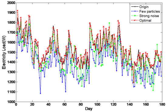
Figure 9.
Particle filter (PF)-based prediction with different parameters.
Table 4.
Performance metrics of particle filter for four seasons with different paraments.
Table 5.
The influence of the number of particles on the computing results.
6. Conclusions
Due to the properties of nonlinear and non-Gaussian distributions, the issue of prediction has always been a difficult problem for electricity load. This also leads to the difficulty of obtaining accurate microgrid operation decisions. To provide accurate load prediction for the microgrid day-ahead scheduling, a PF-based method is proposed in this work. The historical electricity data of Ottawa, Ontario, Canada, for two years is used to certify the accuracy and validity of our proposed PF-based method. Testing and comparing results show that good performance and stability regardless of any time of any seasons. It is noticeable that this superiority is especially clear when compared with the ENN-based method and SVM-based method. Furthermore, an equivalent 44 kV distribution feeder system is utilized to prove the validity and accuracy of PF-based load prediction for distribution system day-ahead scheduling. The results confirmed that by accurately predicting electricity load and robustly providing the scheduled DG power for microgrid operation center, the PF-based predicted method can be an efficient and reliable tool to improve the accuracy and confidence for the decision making in microgrid energy management. Additionally, the performance metrics of particles and the influence of different numbers of particles are discussed. In future work, we will introduce the PF-based algorithm to island microgrids.
Author Contributions
Conceptualization, Q.C. and Y.Y.; writing—original draft preparation; S.L.; methodology, H.C.; supervision, writing—review and editing, C.Y.; writing—review and editing, M.A.; investigation. All authors have read and agreed to the published version of the manuscript.
Funding
This work was supported in part by National Natural Science Foundation of China under Grants 61902168, 61963026, 51765049; in part by Jiangxi Natural Science Foundation under Project 20192BAB215045; in part by Opening Fund of Tianjin Key Laboratory of Civil Aircraft Airworthiness and Maintenance (Civil Aviation University of China).
Conflicts of Interest
The authors declare no conflict of interest.
References
- Rinaldi, S.; Pasetti, M.; Flammini, A.; Ferrari, P.; Sisinni, E.; Simoncini, F. A testing framework for the mon-itoring and performance analysis of distributed energy systems. IEEE Trans. Instrum. Meas. 2015, 68, 3831–3840. [Google Scholar] [CrossRef]
- Farzan, F.; Jafari, M.A.; Masiello, R. Toward optimal day-ahead scheduling and operation control of microgrids under uncertainty. IEEE Trans. Smart Grid 2015, 6, 499–509. [Google Scholar] [CrossRef]
- Ghose, T.; Pandey, H.W.; Gadham, K.R. Risk assessment of microgrid aggregators considering demand response and uncertain renewable energy sources. J. Mod. Power Syst. Clean Energy 2019, 7, 1619–1631. [Google Scholar] [CrossRef]
- Yildiz, B.; Bilbao, J.I.; Sproul, A.B. A review and analysis of regression and machine learning models on commercial building electricity load forecasting. Renew. Sustain. Energy Rev. 2017, 93, 1104–1122. [Google Scholar] [CrossRef]
- Rana, M.; Koprinska, I. Forecasting electricity load with advanced wavelet neural networks. Neurocomputing 2016, 182, 118–132. [Google Scholar] [CrossRef]
- Dash, S.K.; Dash, P.K. Short-term mixed electricity demand and price forecasting using adaptive autoregressive moving average and functional link neural network. J. Mod. Power Syst. Clean Energy 2019, 7, 1241–1255. [Google Scholar] [CrossRef]
- Siddarameshwara, N.; Yelamali, A.; Byahatti, K. Electricity short term load forecasting using elman recurrent neural network. In Proceedings of the 2010 International Conference on Advances in Recent Technologies in Communication and Computing, Kottayam, India, 16–17 October 2010. [Google Scholar]
- Xie, K.; Yi, H.; Hu, G.; Fan, Z. Short-term power load forecasting based on elman neural network with particle swarm optimization. Neurocomputing 2019, 26, 22–59. [Google Scholar] [CrossRef]
- Kelo, S.; Dudul, S. A wavelet elman neural network for short-term electrical load prediction uder the influence of temperature. Int. J. Electr. Power Energy Syst. 2012, 43, 1063–1071. [Google Scholar] [CrossRef]
- Alam, S. Recurrent Neural Networks in Electricity Load Forecasting; Royal Institute of Technolgy: Stockholm, Sweden, 2018. [Google Scholar]
- Zheng, J.; Xu, C.; Zhang, Z.; Li, X. Electric load forecasting in smart grids using long-short-term-memory based recurrent neural network. In Proceedings of the 2017 51st Annual Conference on Information Sciences and Systems (CISS), Baltimore, MD, USA, 22–24 March 2017. [Google Scholar]
- Ugurlu, U.; Oksuz, I.; Tas, O. Electricity price forecasting using recurrent neural networks. Electr. Power Energy Syst. 2018, 11, 1255. [Google Scholar] [CrossRef]
- Ni, K.L.; Wang, J.Z.; Tang, G.Y.; Wei, D.X. Research and application of novel hybrid model based on a deep neural network for electricity load forecasting: A case study in Australia. Energies 2019, 12, 2467. [Google Scholar] [CrossRef]
- Ertugrul, O. Forecasting electricity load by a novel recurrent extreme learning machines approach. Electr. Power Energy Syst. 2016, 78, 429–435. [Google Scholar] [CrossRef]
- Fu, Y.; Li, Z.; Zhang, H.; Xu, P. Using support vector machine to predict next day electricity load of public buildings with sub-metering devices. Procedia Eng. 2015, 121, 1016–1022. [Google Scholar] [CrossRef]
- Ayub, N.; Javaid, N.; Mujeeb, S.; Zahid, M.; Khan, W.Z.; Khattak, M.U. Electricity load forecasting in smart grids using support vector machine. In International Conference on Advanced Information Networking and Applications; Springer: Cham, Switzerland, 2019. [Google Scholar]
- Ma, Z.; Zhong, H.; Xie, L.; Xia, Q.; Kang, C. Month ahead average daily electricity price profile forecasting based on a hybrid nonlinear regression and SVM model: An ERCOT case study. J. Mod. Power Syst. Clean Energy 2018, 6, 281–291. [Google Scholar] [CrossRef]
- Ahmad, W.; Ayub, N.; Ali, T.; Irfan, M.; Awais, M.; Shiraz, M.; Glowacz, A. Towards short term electricity load forecasting using improved support vector machine and extreme learning machine. Energies 2020, 13, 2907. [Google Scholar] [CrossRef]
- Chen, Y.; Xu, P.; Chu, Y.; Li, W.; Wu, Y.; Ni, L.; Bao, Y.; Wang, K. Short-term electrical load forecasting using the support vector regression(svr) model to calculate the demand response baseline for office buildings. Appl. Energy 2017, 195, 659–670. [Google Scholar] [CrossRef]
- Yaslan, Y.; Bican, B. Empirical mode decomposition based denoising method with support vector regression for time series prediction: A case for electricity load forecasting. Measurement 2017, 103, 52–61. [Google Scholar] [CrossRef]
- Badran, R.M.O.; Abdulhadi, E. A fuzzy inference model for short-term load forecasting. Energy Policy 2009, 37, 1239–1248. [Google Scholar]
- Mukhopadhyay, P.; Mitra, G.; Banerjee, S.; Mukherjee, G. Electricity load forecasting using fuzzy logic: Short term load forecasting factoring weather parameter. In Proceedings of the 2017 7th International Conference on Power Systems (ICPS), Pune, India, 21–23 December 2017. [Google Scholar]
- Zhang, J.; Wei, Y.; Li, D.; Tan, Z.; Zhou, J. Short term electricity load forecasting using a hybrid model. Energy 2018, 158, 774–781. [Google Scholar] [CrossRef]
- Wang, D.; Yang, F.; Tsui, K.-L.; Zhou, Q.; Bae, S.J. Remaining useful life prediction of lithium-ion batteries based on spherical cubature particle filter. IEEE Trans. Instrum. Meas. 2016, 65, 1282–1291. [Google Scholar] [CrossRef]
- Yang, C.; Lou, Q.; Liu, J.; Yang, A.Y. Particle filtering-based methods for time to failure estimation with a real-world prognostic application. Appl. Intell. 2018, 48, 2516–2526. [Google Scholar] [CrossRef]
- Li, K.; Wu, J.; Zhang, Q.; Su, L.; Chen, P. New particle filter based on ga for equipment remaining useful life prediction. Sensors 2017, 17, 696. [Google Scholar] [CrossRef]
- Li, L.; Saldivar, A.A.F.; Bai, Y.; Li, Y. Battery remaining useful life prediction with inheritance particle filtering. Energies 2019, 12, 2784. [Google Scholar] [CrossRef]
- Kim, J.; Vaddi, S.S.; Menon, P.K.; Ohlmeyer, E.J. Comparison between nonlinear filtering techniques for spiraling ballistic missile state estimation. IEEE Trans. Aerosp. Electron. Syst. 2012, 48, 313–328. [Google Scholar]
- Nan, X.; Qiu, T.; Li, J.; Li, S. A nonlinear filtering algorithm combining the kalman filter and the particle filter. Acta Electron. Sin. 2013, 41, 148–152. [Google Scholar]
- Rigatos, G.G. Particle filtering for state estimation in nonlinear industrial systems. IEEE Trans. Instrum. Meas. 2019, 58, 3885–3900. [Google Scholar] [CrossRef]
- Liu, S.C.; Liu, P.X.; Wang, X.Y.; Wang, Z.J.; Meng, W.C. Effect of correlated photovoltaic power and load uncertainties on grid-connected microgrid day-ahead scheduling. IET Gener. Transm. Distrib. 2017, 11, 3620–3627. [Google Scholar] [CrossRef]
- Dobos, A.P. Pvwatts Version 5 Manual; NREL: Golden, CO, USA, 2015. [Google Scholar]


Publisher’s Note: MDPI stays neutral with regard to jurisdictional claims in published maps and institutional affiliations. |
© 2020 by the authors. Licensee MDPI, Basel, Switzerland. This article is an open access article distributed under the terms and conditions of the Creative Commons Attribution (CC BY) license (http://creativecommons.org/licenses/by/4.0/).