Leakage Inductances of Transformers at Arbitrarily Located Windings

Abstract

The article presents the calculation of the leakage inductance in power transformers. As a rule, the leakage flux in the transformer window is represented by the short-circuit inductance, which affects the short-circuit voltage, and this is a very important factor for power transformers. This inductance reflects the typical windings of power transformers well, but is insufficient for special transformers or in any case of the internal asymmetry of windings. This paper presents a methodology for calculations of the self- and mutual-leakage inductances for windings arbitrarily located in the air window. It is based on the 2D approach for analyzing the stray field in the air zone only, using discrete partial differential operators. That methodology is verified with the finite element method tested on real transformer data.

1. Introduction

In the long history of research on power transformers, countless books have been published, for example [1,2,3,4,5,6,7]. Theoretically, basic construction and operational problems were solved there. In addition to single-phase and three-phase transformers, new types of special power transformers for power system control, power electronics, and electric and traction have been designed. Two approaches are used to analyze the properties of transformers. The first is based on Maxwell’s field equations. The second is based on Kirchhoff’s equations with mutual-inductances. The field approach is mainly used for transformer design problems, the second for operational problems when the transformer is part of the system. The field approach uses the design data of magnetic circuits and windings, the circuital approach requires relations between the linked fluxes of lumped inductances of the transformer windings and the winding currents. Due to the magnetic non-linearity of the transformer ferromagnetic core, these relations are non-linear, which can only be determined by solving Maxwell’s equations [8,9,10,11,12,13,14,15]. Nowadays, software packages allow us to combine the field and the circuit approaches and calculate output values like currents or voltages at transient or steady-states that are interesting for engineers [16]. However, this is costly and time-consuming and seems inappropriate for solving operational problems in systems with power transformers. Therefore, simplified methods for calculating the lumped parameters of a transformer are often used [17,18,19,20,21,22].

To overcome the difficulties of 2D or 3D non-linear magnetic field computation in the whole transformer magnetic circuit, the relations between linked fluxes ψ_n and currents i_n of elementary windings, which are necessary for the Kirchhoff’s equations of transformers, can be presented in the form:

$$\left[\begin{array}{c}{\psi }_1\\ {\psi }_2\\ ⋮\\ {\psi }_{\mathrm{N}}\end{array}\right]=\left\{\left[\begin{array}{cccc}{\mathrm{L}}_{1,1}^{\mathsf{\mu }}(i)& {\mathrm{L}}_{1,2}^{\mathsf{\mu }}(i)& \cdots & {\mathrm{L}}_{1,\mathrm{N}}^{\mathsf{\mu }}(i)\\ & {\mathrm{L}}_{2,2}^{\mathsf{\mu }}(i)& \cdots & {\mathrm{L}}_{2,\mathrm{N}}^{\mathsf{\mu }}(i)\\ & & \ddots & ⋮\\ (\mathrm{sym})& & & {\mathrm{L}}_{\mathrm{N},\mathrm{N}}^{\mathsf{\mu }}(i)\end{array}\right]+\left[\begin{array}{cccc}{\mathrm{L}}_{1,1}^{\mathsf{\sigma }}& {\mathrm{L}\prime }_{1,2}^{\mathsf{\sigma }}& \cdots & {\mathrm{L}\prime }_{1,\mathrm{N}}^{\mathsf{\sigma }}\\ & {\mathrm{L}\prime }_{2,2}^{\mathsf{\sigma }}& \cdots & {\mathrm{L}\prime }_{2,\mathrm{N}}^{\mathsf{\sigma }}\\ & & \ddots & ⋮\\ (\mathrm{sym})& & & {\mathrm{L}\prime }_{\mathrm{N},\mathrm{N}}^{\mathsf{\sigma }}\end{array}\right]\right\}\left[\begin{array}{c}{i}_1\\ i_2\\ ⋮\\ i_{\mathrm{N}}\end{array}\right]i=\{i_1,i_1,\dots ,i_{\mathrm{N}}\}$$

(1)

The above two matrices can be calculated separately using a simplified method. The first matrix has inductances, due to fluxes in the core, and the second one results from the leakage field in the transformer windows. Inductances ${\mathrm{L}}_{n,m}^{\mathsf{\mu }}(i)$ are non-linear, taking into account the saturation of the ferromagnetic core, and may depend on all winding currents. This matrix can be determined using circuit representation of ferromagnetic core with non-linear lumped parameters, omitting fluxes in the air. The second matrix, containing the leakage inductances, can be found taking into account only the window zone and assuming that ${\mathsf{\mu }}_{\mathrm{Fe}}\to \infty$. The leakage inductances ${\mathrm{L}}_{n,m}^{\mathsf{\sigma }}$ are constant because the window zone is magnetically linear.

For symmetrically designed power transformers, with magnetic circuits and winding locations sketched in Figure 1, the matrices in (1) take extremely simple forms, which are well known from books and textbooks. Commonly, those matrices are determined by three lumped parameters: Non-linear magnetizing inductance ${\mathrm{L}}_{\mathsf{\mu }}^{}(i_{\mathsf{\mu }}^{})$ and two leakage inductances of primary ${\mathrm{L}}_{\mathrm{p}}^{\mathsf{\sigma }}$ and secondary winding ${\mathrm{L}}_{\mathrm{s}}^{\mathsf{\sigma }}$. The inductance ${\mathrm{L}}_{\mathsf{\mu }}^{}(i_{\mathsf{\mu }}^{})$ represents relation between the linked flux in the limb and the magnetizing current. The sum of leakages inductances determines the short-circuit inductance ${\mathrm{L}}_{\mathrm{sc}}^{}$, and consequently, the short-circuit voltage. It is a very important technical parameter of power transformers. The short-circuit inductance is calculated from the magnetic field in the transformer window with two windings on the same limb, assuming that the ampere-turn compensates and the magnetic permeability of the ferromagnetic core is sufficiently high. The field analysis in the 1D transformer window model provides rather simple formulae for the short circuit inductance. This can be found in books on transformers, and is still recommended for designers. The leakage inductances ${\mathrm{L}}_{\mathrm{p}}^{\mathsf{\sigma }}$ and ${\mathrm{L}}_{\mathrm{s}}^{\mathsf{\sigma }}$ are not calculated, but estimated based on the short circuit inductance [19,20], often just by dividing the short-circuit inductance by 2. This approach is sufficient for symmetrically located windings, when they cover, more or less, the limbs, and the Rogowski factor can correct the length of the magnetic field path in the air. Figure 2a illustrates such a case. Figure 2b shows the position of windings when HV windings are modified, for voltage regulation purposes, by eliminating some numbers of turns in the middle part. Figure 3a presents a case when a short circuit in the HV winding in phase ‘A’ arise. For the cases ‘b’ and ‘c’ leakage inductances cannot be estimated from 1D field analysis.

Rectifier transformers for multi-phase voltages and currents [7] can have windings that are much shorter than the limb’s height, and the Rogowski factor cannot be applied. Figure 2a shows an example of the location of the windings in the transformer window for Yyd 3/6-phase transformers for 12 pulses rectifiers and Figure 2b for Y_zyd 3/12-phase transformers for 24 pulses rectifiers. The position of the windings loses the characteristic symmetry for classic three-phase power transformers, see Figure 1. At least the 2D field is necessary to find leakage inductances.

An analytical solution of the magnetic vector potential in transformer air windows with arbitrarily located balanced pairs of windings is presented in [21]. The zero Neumann boundary conditions can be stated for such cases on the ferromagnetic boundaries, which means that the magnetizing current is omitted. We can then calculate the short circuit inductance for any pair of windings. However, this approach cannot be used to determine the leakage inductances of individual windings and the mutual-inductances caused by the stray field. To find these inductances, 2D or 3D field calculations are typically needed, including the entire magnetic circuit with the ferromagnetic core and the air zone. [11,12,13,14,15,22,23].

This paper presents a 2D numerical approach for determining all leakage inductances ${\mathrm{L}}_{n,m}^{\mathsf{\sigma }}$, both self, as well as mutual, for arbitrarily located windings considering the magnetic field in the air window only, when surrounded by ferromagnetic walls with high permeability. Difficulties in formulating the boundary conditions for the case of one winding in the air window has been omitted based on the results of test calculations using the 2D Finite Element Method (FEM). Ferromagnetic plates with sufficiently high magnetic permeability around the air window have been included for that calculations at zero Dirichlet condition on external boundaries. To fulfill the conditions that were followed for those tests, additional ampere-turns have been added at the boundaries. It allowed us to obtain the magnetic vector potential distribution in the air window area the same as form the FEM method, with sufficiently good accuracy. Self- and mutual-leakage inductances can be calculated using an energy approach. This time, however, each pair of windings is represented by two self-inductances and one mutual-inductance instead of one short-circuit inductance. In this way, it is possible to determine all elements of the leakage induction matrix in equation ((1)). When the elementary windings are connected, constituting the final transformer’s windings, the matrix of constraints $C$ can be defined and the final inductance matrix takes the form,

$$L=C^T\cdot (L_{\mathsf{\mu }}+L_{\mathsf{\sigma }})\cdot C$$

(2)

The paper is organized as follows: In the second section, numerical tests are presented, leading to a formulation of boundary conditions on ferromagnetic walls on the air window for unbalanced ampere-turns in the air window. For this purpose, the 2D FEM has been applied. In Section 3, the finite-difference equations have been formulated for magnetic potential in 2D air zone using the Discrete Partial Differential Operators (DPDO), which are presented in Appendix A. Results have been compared to those from FEM, confirming satisfactory accuracy. Section 4 presents energy-based calculations of self- and mutual-inductances, due to fluxes in the air window. The results for two cases: Windings typical location of a three phase power transformers and for short-circuited part of a winding are presented in Section 5. Finally, conclusions are given in Section 6.

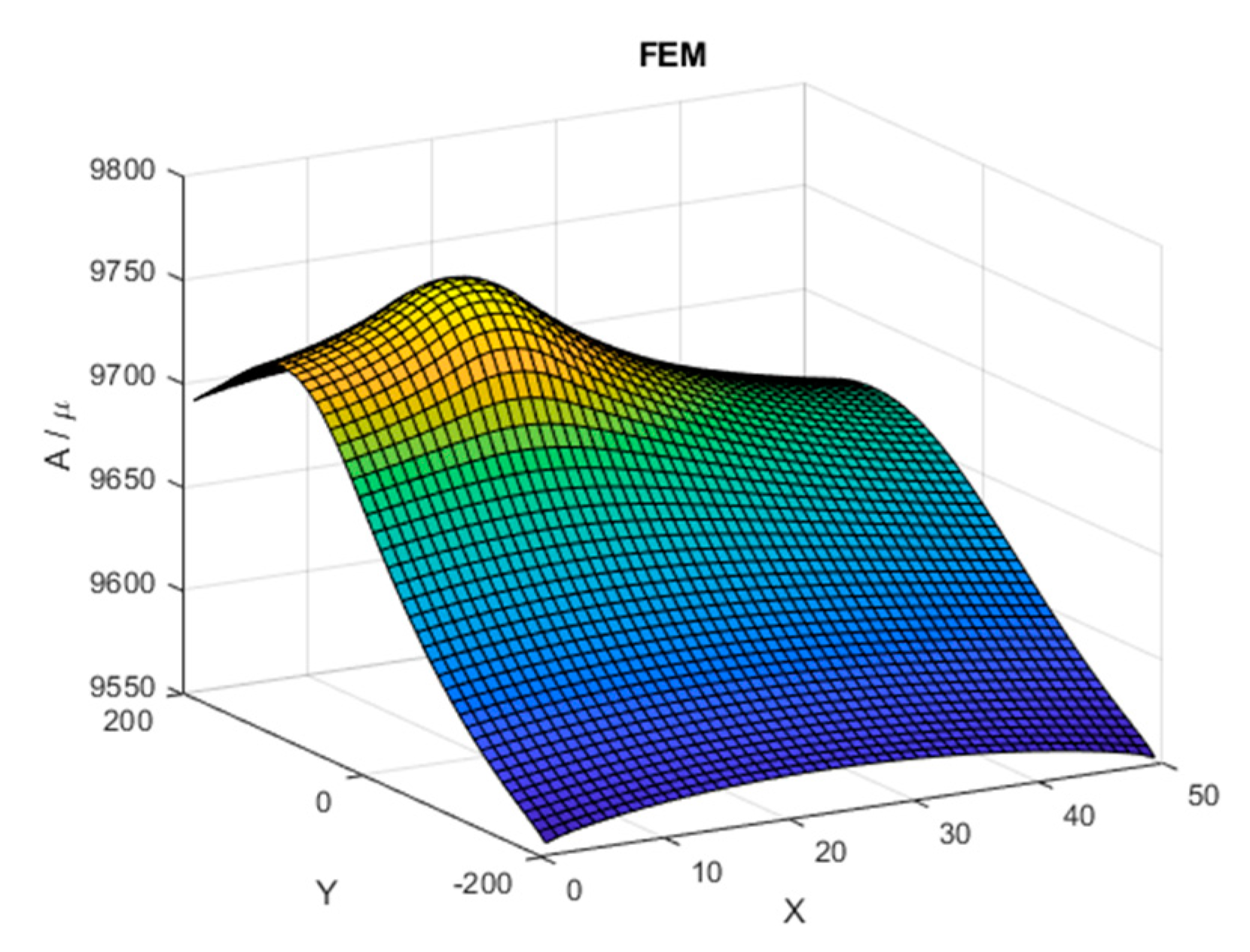
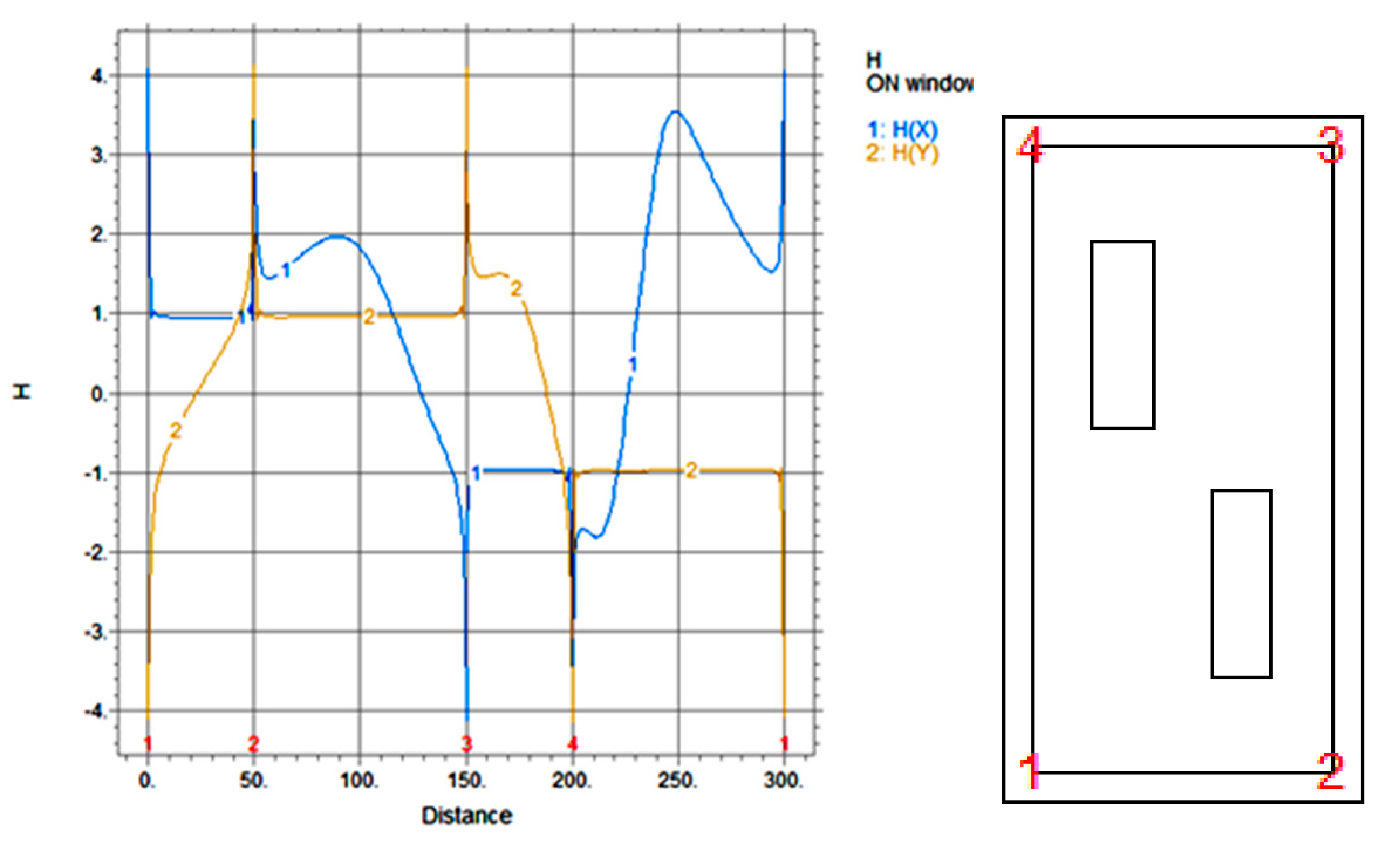
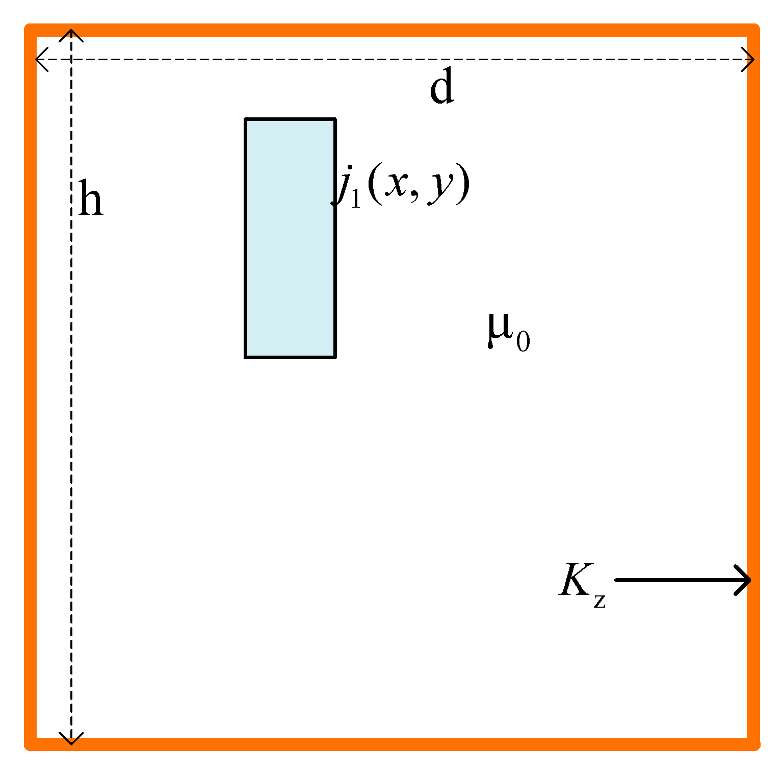
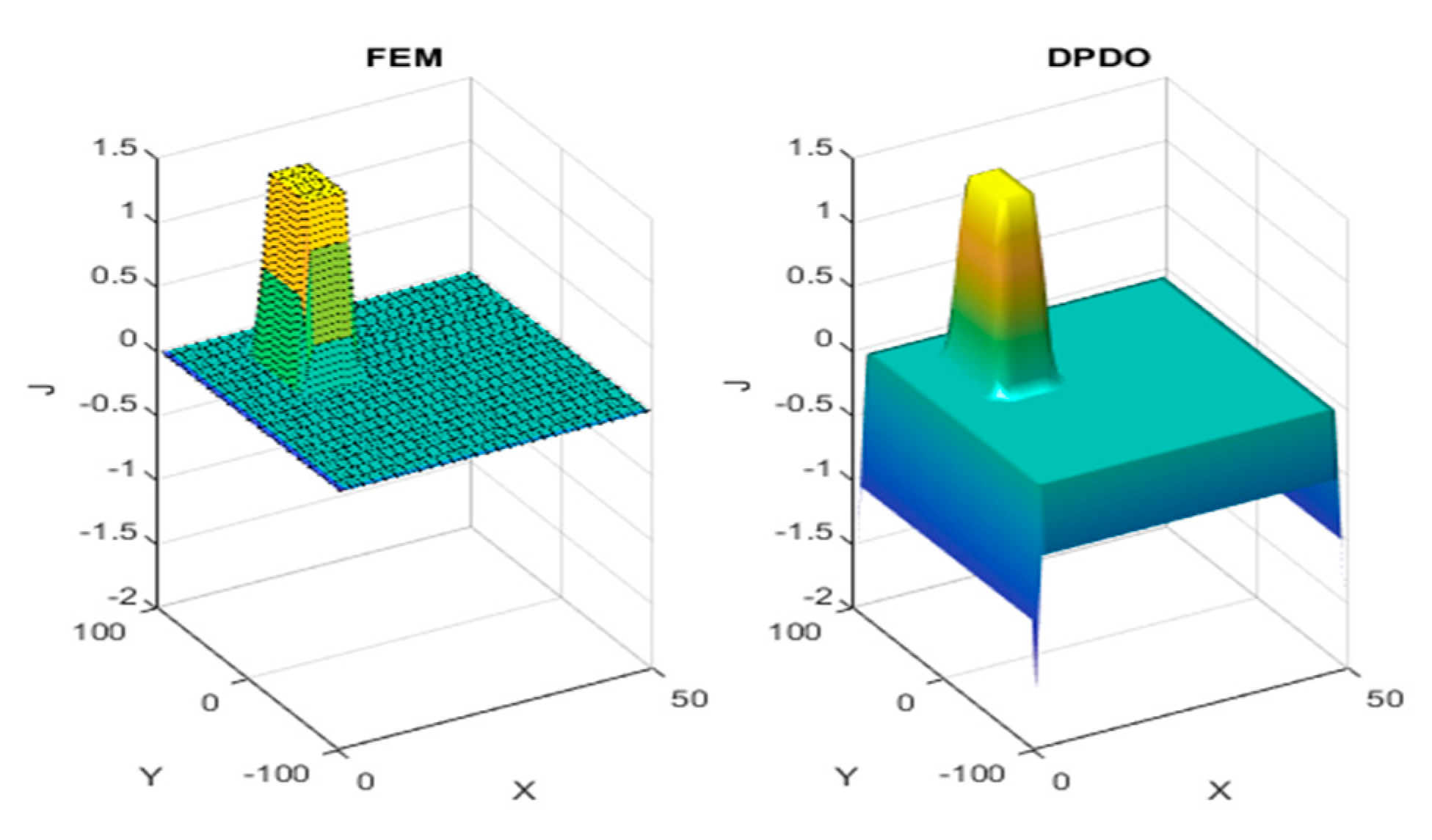
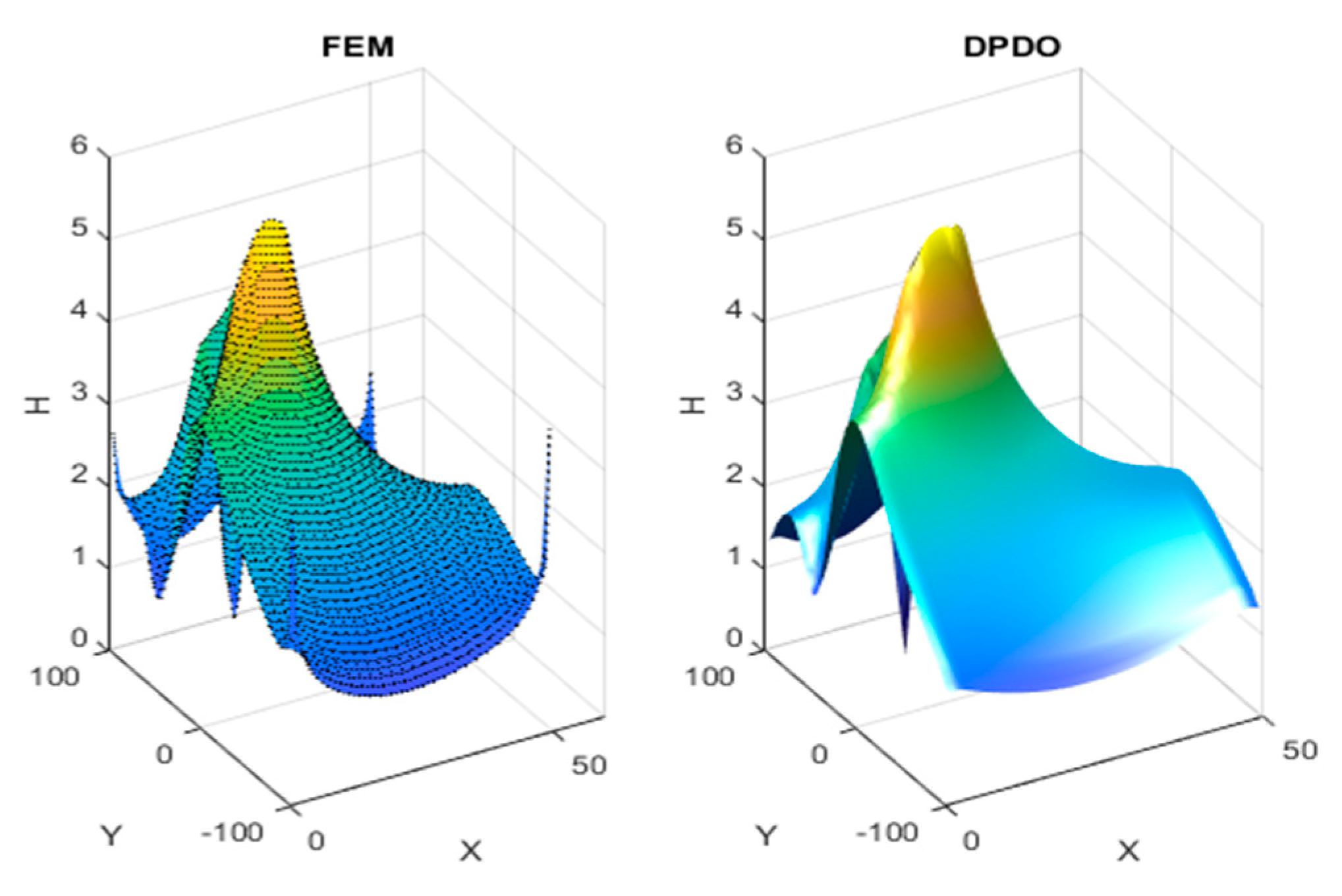
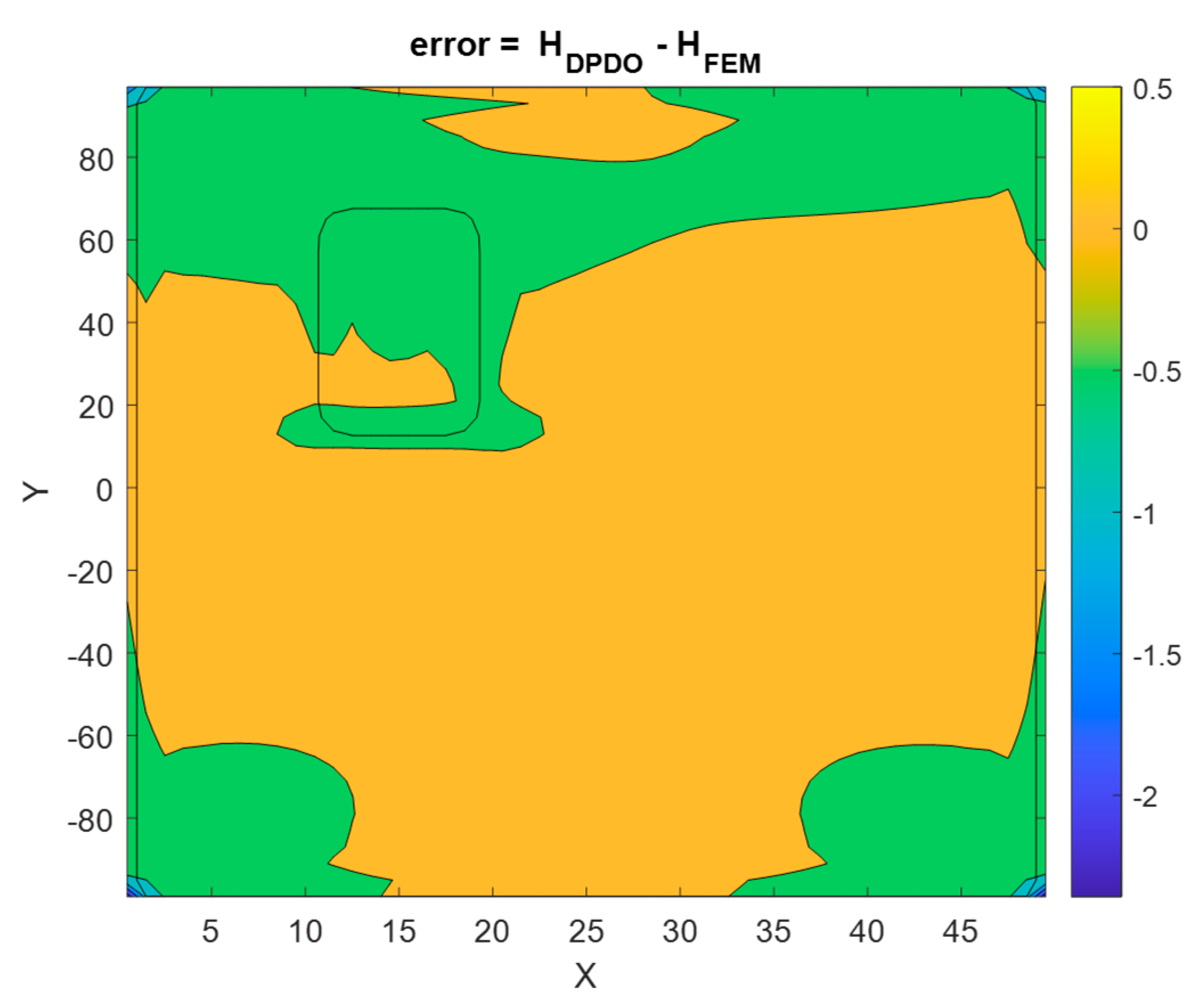
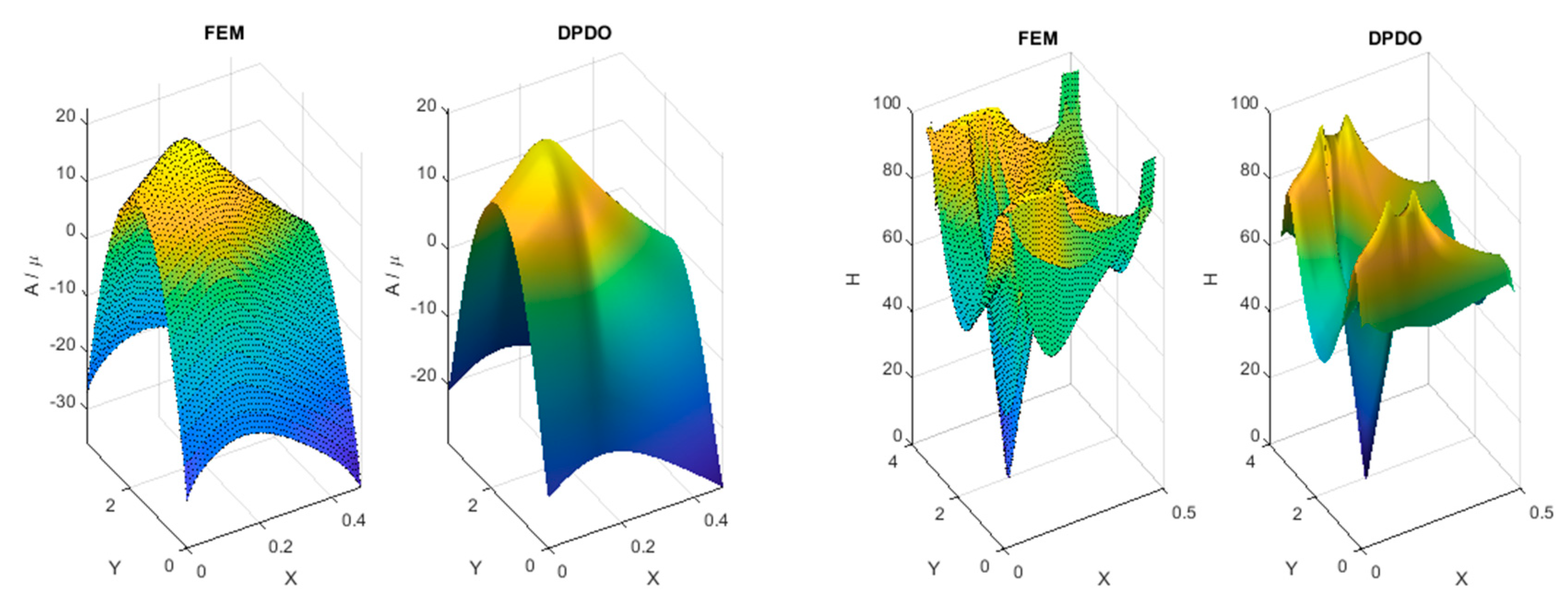
2. Calculations of Magnetic Field in the Transformer’s Air Window with FEM

To determine the leakage inductance matrix $L_{\mathsf{\sigma }}$, the self- and mutual-inductances for each pair of windings should be calculated. As an example, a pair of arbitrarily located windings is illustrated in Figure 4.

Calculation of self-inductances is not a trivial problem because the magnetic field in the air window zone should be generated by one winding only, omitting a magnetic core. It is not possible to formulate the boundary conditions for the equation of the magnetic potential for such a case, as it has been explained in [24]. In 2D, the magnetic potential in the air window is described by the partial differential equation of the form:

$$\frac{{\partial }^{2}A(x,y)}{\partial x^2}+\frac{{\partial }^{2}A(x,y)}{\partial y^2}=-{\mathsf{\mu }}_0\left(j_1(x,y)+j_2(x,y)\right)$$

(3)

where $A(x,y)$ is the magnetic potential, $j_1(x,y)$ and $j_2(x,y)$ are ampere-turns densities of respective windings. The windings with currents $i_1$ and $i_2$ have numbers of turns ${\mathrm{w}}_1$ and ${\mathrm{w}}_2$ respectively. Taking into account the ferromagnetic, the zero Dirichlet conditions can be determined on the external circumference of the ferromagnetic core. However, by omitting the ferromagnetic core, i.e., assuming ${\mathsf{\mu }}_{\mathrm{Fe}}=\infty$, it is not possible to formulate the boundary conditions only for the air window. The zero Neumann conditions are applicable only in the case of balanced ampere-turns ${\mathrm{w}}_1\cdot i_1+{\mathrm{w}}_2\cdot i_2=0$ [23]. To determine the boundary conditions for non-balanced ampere-turns in the transformer window, some numeric test was carried out. The magnetic potential was calculated for the case when only one winding exists in the air window, i.e., ${\mathrm{w}}_2\cdot i_2=0$, but the ferromagnetic walls are included too. The 2D finite elements software has been used here, assuming zero Dirichlet conditions at the outer boundaries of the ferromagnetic core. The permeability of ferromagnetic ${\mathsf{\mu }}_{\mathrm{Fe}}$ have been rising up to $10 000\cdot {\mathsf{\mu }}_0$ in successive calculations. Figure 5 shows the magnetic potential distribution $A(x,y)$ in the air zone only when one winding generates the field at the highest value of magnetic permeability ${\mathsf{\mu }}_{\mathrm{Fe}}$.

Figure 6 presents the components of the magnetic field $H_{\mathrm{x}}\left(x,y\right)$ and $H_{\mathrm{y}}\left(x,y\right)$ along boundaries of the air window, where

$$H_{\mathrm{x}}\left(x,y\right)=\frac{1}{{\mathsf{\mu }}_0}\frac{\mathrm{d}}{\mathrm{d}y}A\left(x,y\right) H_{\mathrm{y}}\left(x,y\right)=-\frac{1}{{\mathsf{\mu }}_0}\frac{\mathrm{d}}{\mathrm{d}x}A\left(x,y\right)$$

Results of FEM calculations show that the tangential components $H_{\mathrm{t}}$ of a magnetic field on the air window boundaries keep constant values. Its value can be determined from the integral form of the Maxwell equation,

$${\displaystyle \underset{l}{\oint }{H}_{\mathrm{t}}\mathrm{d}l}={\displaystyle \underset{S}{\iint }j(x,y)\mathrm{d}x\mathrm{d}y}$$

(4)

The curve $\prime l\prime$ is the circumference of the air window and $\prime S\prime$ is the surface limited by this curve. The value of that component equals ${\mathrm{H}}_{\mathrm{t}}={\mathrm{w}}_1\cdot i_1/(2\cdot (\mathrm{h}+\mathrm{d}))$ in considered case.

In this paper it is proposed to modify the ampere-turns function in the air window instead of solving the Equation (3) with zero Neumann boundary conditions when omitting $j_2(x,y)$. This modification results in ampere-turns that are now balanced. To eliminate the ferromagnetic core from the computation a general formula for tangential components on both sides of the boundary $H_t^{air}-H_t^{Fe}=0$ has been changed to $H_t^{air}-0=K_{\mathrm{z}}$, where $K_{\mathrm{z}}$ is a surface current in $\prime z\prime$ direction, which equals to the constant component ${\mathrm{H}}_{\mathrm{t}}$ found using FEM

$$K_{\mathrm{z}}={\mathrm{H}}_{\mathrm{t}}={\mathrm{w}}_1\cdot i_1/(2(\mathrm{h}+\mathrm{d}))$$

(5)

That additional surface current is located on the air window boundary, as it is presented in Figure 7.

The exciting function is now balanced and satisfies the relation,

$${\displaystyle \underset{\begin{array}{l}0<x<2\mathsf{\pi }\\ 0<y<2\mathsf{\pi }\end{array}}{\iint }{j}_1(x,y) \mathrm{d}x \mathrm{d}y}={\displaystyle \underset{\begin{array}{l}0<x<2\mathsf{\pi }\\ 0<y<2\mathsf{\pi }\end{array}}{\iint }\nabla \cdot \overrightarrow{K}(x,y) \mathrm{d}x \mathrm{d}y}$$

(6)

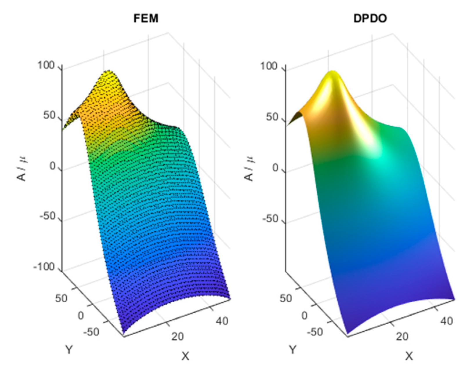
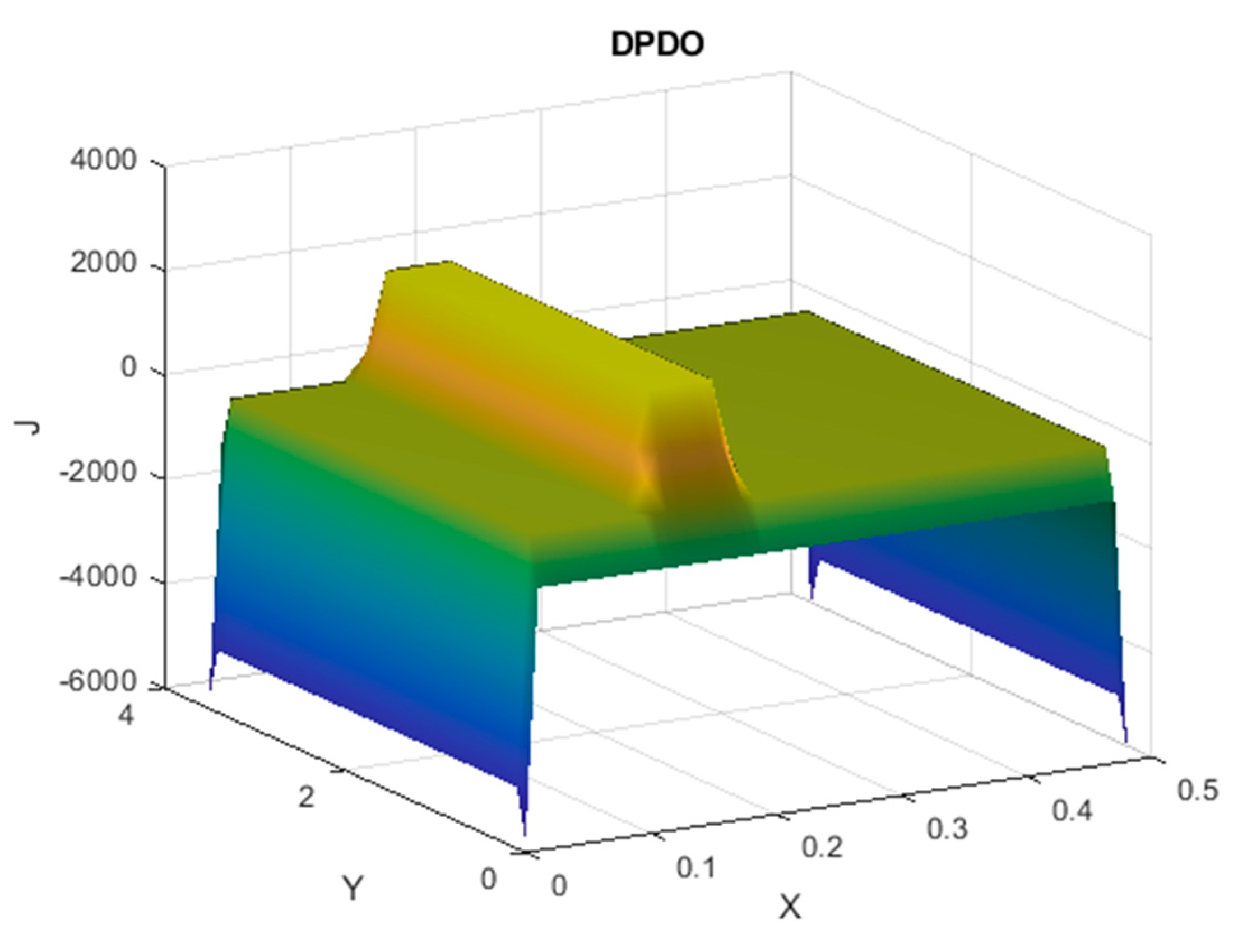
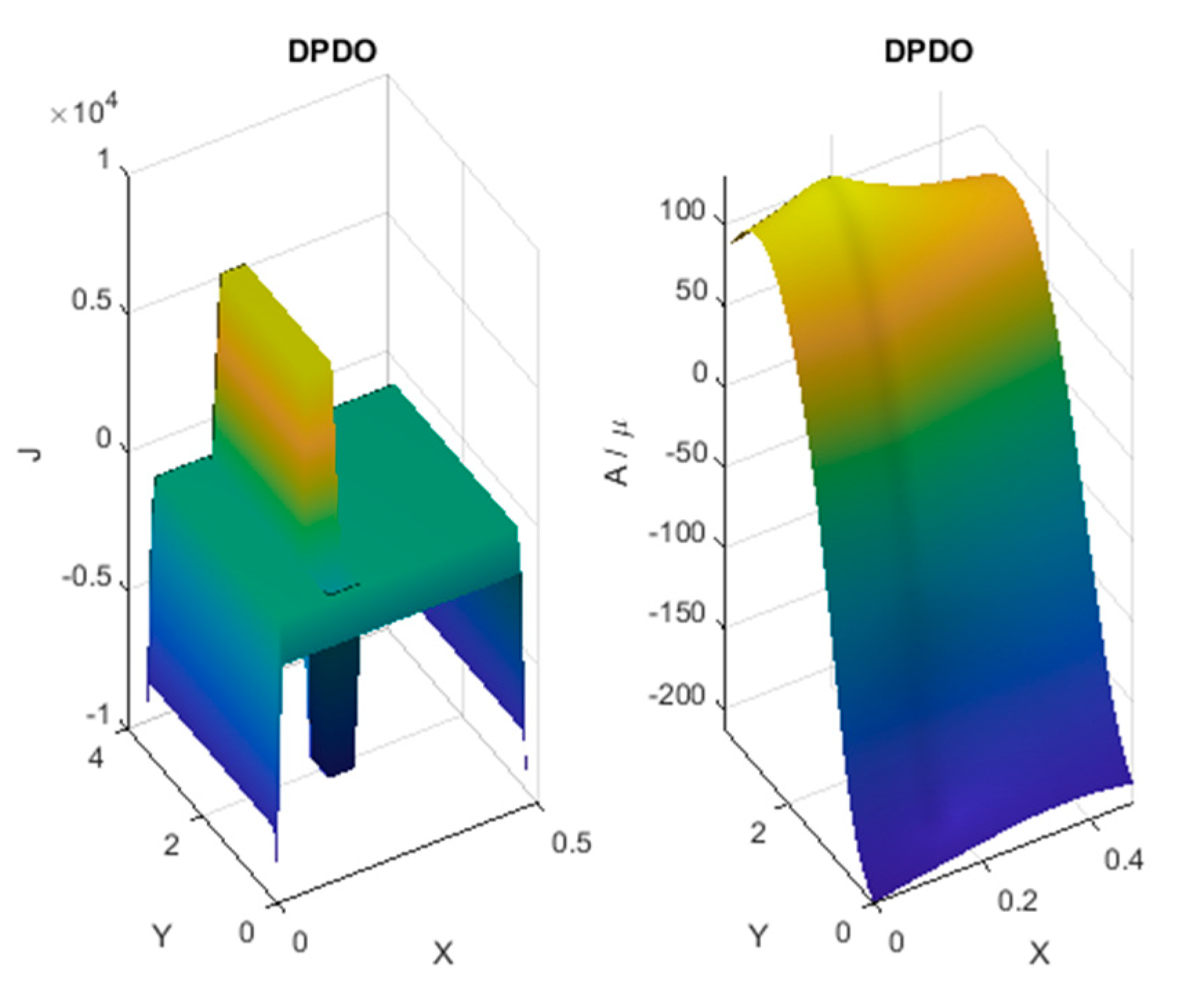
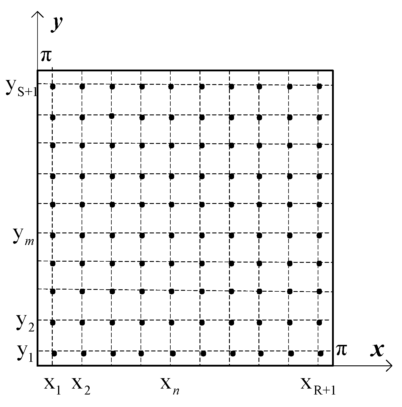
3. Calculations of Magnetic Field in the Transformer Air Window using PDPO

The equation with a modified excitation has the form,

$$\left(\frac{{\partial }^{2}A(x,y)}{\partial x^2}+\frac{{\partial }^{2}A(x,y)}{\partial y^2}\right)=-{\mathsf{\mu }}_0\cdot \left(j_{\mathrm{mod}}(x,y)\right)$$

(7)

where

$$j_{\mathrm{mod}}(x,y)=j_1(x,y)-\frac{\partial K_{\mathrm{z}}(x,y)}{\partial x}-\frac{\partial K_{\mathrm{z}}(x,y)}{\partial y}$$

and can be solved for zero Neumann conditions at all boundaries. The modified excitation is compared to the windings ampere-turn function in Figure 8.

The solution of that equation can be predicted in the form of the double Fourier series of cosine functions [24],

$$A(x,y)={\displaystyle \sum _{r=0}^{\infty }{\displaystyle \sum _{s=0}^{\infty }{\mathrm{A}}_{r,s}\cdot \left(\cos (r\cdot \mathsf{\pi }\cdot \frac{x}{\mathrm{d}})\cdot \cos (s\cdot \mathsf{\pi }\cdot \frac{x}{\mathrm{h}})\right)}}\mathrm{at} {\mathrm{A}}_{0,0}\equiv 0$$

(8)

The function $j_{\mathrm{mod}}(x,y)$ is rather inconvenient for the Fourier analysis, so to solve Equation (6) a special numerical approach has been applied. To find the magnetic potential the DPDO [25,26] have been developed for the series (8). Full consideration leading to the DPDO are presented in Appendix A. The DPDO have been successfully applied for solving 1D boundary problems [24,25,26].

The Finite-Difference Equations (FDE) can be rather easily written using DPDO operators, and it takes the form,

$${\mathsf{\mu }}_0\cdot D_{}^{(2)}\cdot A=-J \mathrm{where} D_{}^{(2)}=(D_{\mathrm{xx}}^{(2)}+D_{\mathrm{yy}}^{(2)})$$

(9)

The vectors $A$ and $J$ are composed like vectors $z$ and $g$ in Appendix A. The matrix $D_{}^{(2)}$ is singular and has only one eigenvalue equal to zero, so its rank is $\left(\right(\mathrm{R}+1)\cdot (\mathrm{S}+1)-1)$. As it has been mention before the series should satisfy the condition ${\mathrm{A}}_{0,0}=0$, i.e.,

$${\displaystyle \sum _{n=1}^{\mathrm{R}+1}{\displaystyle \sum _{m=1}^{\mathrm{S}+1}{\mathrm{A}}_{n,m}=0}}$$

(10)

It is, in fact, the constraint equation for the elements of the vector $A$, which can be expressed in the form:

$$A=\left[\begin{array}{c}{\mathrm{A}}_{1,1}\\ {\mathrm{A}}_{1,2}\\ ⋮\\ {\mathrm{A}}_{\mathrm{R}+1,\mathrm{S}+1}\end{array}\right]=\left[\begin{array}{ccc}-1& \cdots & -1\\ 1& & \\ & \ddots & \\ & & 1\end{array}\right]\left[\begin{array}{c}{\mathrm{A}}_{1,2}\\ ⋮\\ {\mathrm{A}}_{\mathrm{R}+1,\mathrm{S}+1}\end{array}\right]=C\cdot A_{\mathrm{C}}$$

(11)

where $C$ is the constraint matrix. Finally, the FDEs can be written in the form,

$${\mathsf{\mu }}_0\cdot \left(C^T\cdot D_{}^{(2)}\cdot C\right)\cdot A_{\mathrm{C}}=-C^T\cdot J$$

(12)

The matrix $C^T\cdot D_{}^{(2)}\cdot C=D_{\mathrm{C}}^{(2)}$ is non-singular, and the new FDEs (12) have a unique solution.

The algorithm for solving the FDE (12) has been prepared in MATLAB, and the resulting magnetic potential distribution in the air window area is presented in Figure 9, denoted as DPDO. These results are compared to the results of FEM with a reduced mean value to zero.

The magnetic field distribution,

$$H(x,y)=\sqrt{{(H_{\mathrm{x}}(x,y))}^2+{(H_{\mathrm{y}}(x,y))}^2}$$

(13)

has been determined based on $A(x,y)$. The first order DPDO has been used for that.The results, both of FEM and DPDO, are shown in Figure 10.

The differences between solutions of magnetic field distributions are presented in Figure 11 and seem to be sufficiently small.

and the solution can be predicted as the Fourier series (7). Application of the DPDO leads to the required solution.

4. Co-Energy Based Calculations of Self- and Mutual-Leakage Inductances

The inductances ${\mathrm{L}}_{n,n}^{\mathsf{\sigma }}$, ${\mathrm{L}}_{m,m}^{\mathsf{\sigma }}$, and ${\mathrm{L}}_{n,m}^{\mathsf{\sigma }}$ in the Formula (1) can be calculated based on field distribution in the air window, obtained with application of the second order DPDOs presented in Appendix A. Two formulae of magnetic co-energy stored in the air can be used here. The first one determines co-energy from the distribution of the magnetic field:

$${\mathrm{E}}_{\mathrm{co}}=\frac{1}{2}{\displaystyle \underset{V}{\iiint }(\overrightarrow{B} \cdot \overrightarrow{H}) \mathrm{d}V}$$

(14)

and the second is based on lumped inductances of coils,

$${\mathrm{E}}_{\mathrm{co}}=\frac{1}{2}{\mathrm{L}}_{n,n}^{\mathsf{\sigma }}\cdot {(i_n)}^2+\frac{1}{2}{\mathrm{L}}_{m,m}^{\mathsf{\sigma }}\cdot {(i_m)}^2+{\mathrm{L}}_{n,m}^{\mathsf{\sigma }}\cdot i_n\cdot i_m$$

(15)

Inductances can be calculated in three steps:

-

Calculate inductance ${\mathrm{L}}_{n,n}^{\mathsf{\sigma }}$ from the co-energy ${\mathrm{E}}_{\mathrm{co},n}$ at $i_n={\mathrm{I}}_n$ and $i_m=0$,

$${\mathrm{E}}_{\mathrm{co},n}=\frac{1}{2}{\mathrm{L}}_{n,n}^{\mathsf{\sigma }}\cdot {({\mathrm{I}}_n)}^2$$

(16)

-

Calculate inductance ${\mathrm{L}}_{m,m}^{\mathsf{\sigma }}$ from the co-energy ${\mathrm{E}}_{\mathrm{co},\mathrm{m}}$ at $i_n=0$ and $i_m={\mathrm{I}}_m$,

$${\mathrm{E}}_{\mathrm{co},m}=\frac{1}{2}{\mathrm{L}}_{m,m}^{\mathsf{\sigma }}\cdot {({\mathrm{I}}_m)}^2$$

(17)

-

Calculate inductance ${\mathrm{L}}_{m,m}^{\mathsf{\sigma }}$ from the co-energy ${\mathrm{E}}_{\mathrm{co},nm}$ at $i_n={\mathrm{I}}_{\mathrm{n}}$ and $i_m={\mathrm{I}}_m$,

$${\mathrm{E}}_{\mathrm{co}}-{\mathrm{E}}_{\mathrm{co},\mathrm{n}}-{\mathrm{E}}_{\mathrm{co},m}={\mathrm{L}}_{m,m}^{\mathsf{\sigma }}\cdot {\mathrm{I}}_n\cdot {\mathrm{I}}_m$$

(18)

In 2D the formula of the co-energy takes the form,

$$E_{\mathrm{co}}=\frac{1}{2}{\mathsf{\mu }}_0\cdot {\mathrm{l}}_{eq}\cdot {\displaystyle \underset{0}{\overset{\mathrm{h}}{\int }}{\displaystyle \underset{0}{\overset{\mathrm{d}}{\int }}\left({\left(H_{\mathrm{x}}(x,y)\right)}^2+{\left(H_{\mathrm{y}}(x,y)\right)}^2\right)\mathrm{d}x\mathrm{dy}}}$$

(19)

where ${\mathrm{l}}_{eq}$ is an equivalent length of the air window in z-direction, usually it is the circumference taken in the middle of the air window.

5. Results of Teste Calculations

5.1. Test 1

As the first test, the leakage inductance matrix $L_{\mathsf{\sigma }}$ of a typical power transformer has been determined. The transformer is shown schematically in Figure 1. The inductance matrix can be predicted in the form

$$L_{\mathsf{\sigma }}=\left[\begin{array}{cccccc}{\mathrm{L}}_{1,1}^{\mathsf{\sigma }}& {\mathrm{L}}_{1,2}^{\mathsf{\sigma }}& 0& {\mathrm{L}}_{1,4}^{\mathsf{\sigma }}& {\mathrm{L}}_{1,5}^{\mathsf{\sigma }}& 0\\ & {\mathrm{L}}_{2,2}^{\mathsf{\sigma }}& {\mathrm{L}}_{2,3}^{\mathsf{\sigma }}& {\mathrm{L}}_{2,4}^{\mathsf{\sigma }}& {\mathrm{L}}_{2,5}^{\mathsf{\sigma }}& {\mathrm{L}}_{2,6}^{\mathsf{\sigma }}\\ & & {\mathrm{L}}_{3,3}^{\mathsf{\sigma }}& 0& {\mathrm{L}}_{3,5}^{\mathsf{\sigma }}& {\mathrm{L}}_{3,6}^{\mathsf{\sigma }}\\ & & & {\mathrm{L}}_{4,4}^{\mathsf{\sigma }}& {\mathrm{L}}_{4,5}^{\mathsf{\sigma }}& 0\\ & (\mathrm{sym})& & & {\mathrm{L}}_{5,5}^{\mathsf{\sigma }}& {\mathrm{L}}_{5,6}^{\mathsf{\sigma }}\\ & & & & & {\mathrm{L}}_{6,6}^{\mathsf{\sigma }}\end{array}\right]$$

Design data, more or less related to a power transformer of about 60MVA, 110/60kV, Yd11 have been used for calculations. Its air window and the winding locations are shown in Figure 12, keeping the proportions. The following data are used for computations: Air window dimensions $\mathrm{h}=1750 \mathrm{mm}$, $\mathrm{d}=480 \mathrm{mm}$, diameter of limbs ${\mathrm{d}}_{\mathrm{limb}}=580\mathrm{mm}$. The equivalent length of widows in z-direction equals to circumference of a circle of a diameter ${\mathrm{l}}_{\mathrm{e}\mathrm{q}}=\mathrm{p}\cdot (580+480)\mathrm{m}\mathrm{m}$. The winding’s dimensions are: HV−${\mathrm{h}}_1=1550 \mathrm{mm}$, ${\mathrm{d}}_1=70 \mathrm{mm}$, LV-${\mathrm{h}}_2=1650 \mathrm{mm}$,${\mathrm{d}}_2=50 \mathrm{mm}$ and the distance between HV and LV windings is $\mathsf{\delta }=30\mathrm{mm}$. Numbers of turns are: HV–720 and LV–240.

The magnetic vector potential in the air window has been determined by solving equation (12) using the second order DPDO, presented in Appendix A. The modified ampere-turn functions have been determined for individual cases. An exemplary winding ‘1′ is presented in Figure 13. The magnetic field distribution in the air window has been obtained using the first order DPDO. The discretization mesh, with $\Delta \mathrm{x}=10 \mathrm{mm}$ and $\Delta \mathrm{y}=50 \mathrm{mm}$ has been chosen, i.e., the number of points in $x$’ direction is 49 and in $y$ direction is 36, which leads to 1764 points in the whole area. The leakage inductances have been obtained from equalities (14)–(16) for an arbitrary value of currents.

Figure 14 presents distributions of magnetic potential $A(x,y)$ and magnetic field $H(x,y)$ in the air window obtained from FEM and the DPDO.

The components of magnetic field $H_{\mathrm{x}}(x,y)$ and $H_y(x,y)$ are shown in Figure 15. The value of $H_{\mathrm{x}}(x)$ on the boundaries in direction $x$ is constant and equals ${\mathrm{H}}_{\mathrm{x}}=\pm 50\mathrm{A}/\mathrm{m}$ and $H_{\mathrm{y}}(y)$ on the boundaries in direction $y$ is constant also and equals ${\mathrm{H}}_{\mathrm{y}}=\pm 50\mathrm{A}/\mathrm{m}$.

The values of leakage inductances have been calculated using relations (14)–(16) for the number of turns of HV winding ‘1′. The inductance values are presented in the matrix below. The symmetry of windings has been taken into account, which is reflected in matrix structure.

$$L_{\mathsf{\sigma }}=\left[\begin{array}{cccccc}\begin{array}{r}\hfill 203.06\end{array}& 93.21& 0& 153.41& 30.07& 0\\ & 203.06& 93.21& 31.10& 153.41& 30.07\\ & & 203.06& 0& 31.10& 153.41\\ & & & 195.95& -26.74& 0\\ & (sym)& & & 195.95& -26.74\\ & & & & & 195.95\end{array}\right]\cdot {10}^{-3}\mathrm{H}$$

The short circuit inductance, when accounting for the couplings between the windings on the same limb only, equals ${\mathrm{L}}_{\mathrm{sc}}=82.19 \mathrm{mH}$. The same matrix calculated from expressions presented in [24], obtained in 1D approach, has the form,

$$L_{\mathsf{\sigma }}=\left[\begin{array}{cccccc}134.20& 30.97& 0& 92.91& -24.78& 0\\ & 134.20& 30.97& -24.78& 92.91& -24.78\\ & & 134.20& 0& -24.78& 92.91\\ & & & 138.33& -80.52& 0\\ & (sym)& & & 138.33& -80.52\\ & & & & & 138.33\end{array}\right]\cdot {10}^{-3}\mathrm{H}$$

The corresponding short circuit impedance equals L_sc = 86.72 mH. The differences between those matrices seem to be rather high, but the short circuit inductances are almost equal.

5.2. Test 2

For the second test, the leakage inductance matrix has been determined when the short circuit of a part of HV winding occurs, as it is presented in Figure 16. The same data as for Test 1 have been assumed, but 20% of HV winding is short circuited. For that test, the other windings have been omitted. For that case, the leakage inductance matrix takes the form,

$$L_{\mathsf{\sigma }}=\left[\begin{array}{ccc}{\mathrm{L}}_{1,1}^{\mathsf{\sigma }}& {\mathrm{L}}_{1,2}^{\mathsf{\sigma }}& {\mathrm{L}}_{1,\mathrm{sc}}^{\mathsf{\sigma }}\\ & {\mathrm{L}}_{2,2}^{\mathsf{\sigma }}& {\mathrm{L}}_{\mathrm{sc},2}^{\mathsf{\sigma }}\\ (sym)& & {\mathrm{L}}_{\mathrm{sc}}^{\mathsf{\sigma }}\end{array}\right]$$

and values of respective inductances are,

$$L_{\mathsf{\sigma }}=\left[\begin{array}{ccc}229.84& 47.31& -44.22\\ & 21.78& 5.38\\ (\mathrm{sym})& & 66.80\end{array}\right]$$

These inductances cannot be found from a 1D approach. To confirm it, the magnetic potential distribution in the short circuit coil case is shown in Figure 17.

6. Conclusions

This paper presented a method for calculations of self- and mutual-leakage inductances of power transformer windings with arbitrary winding locations in the air windows. It was possible to obtain inductance values based on 2D calculations of the magnetic field only in the air zone, using discrete partial differential operators for 2D periodic functions. The boundary conditions which allowed for the elimination of the transformer ferromagnetic core were determined based on the test calculations of the magnetic field distribution using FEM that included a transformer core of sufficiently high permeability. It followed that the surface current should be located on the boundaries.

To find the solution predicted in the air zone, the discrete partial differential operators of the first- and the second orders have been developed and presented in Appendix A. They allowed us to easily create the finite-difference equations determining the 2D magnetic vector potential distribution in the air window, and consequently, the distribution of the magnetic field strength. The results are sufficiently accurate comparing to FEM.

The energy-based method has been successfully used to calculate the leakage inductances, both the self- and mutual-inductances. The matrix of such inductances has been calculated for the design data of a real three-phase power transformer. For a case when a part of one winding on one limb is short circuited, the inductances have also been calculated.

References

1. Arnold, E.; la Cour, J.L. Die Transformatoren; Springer: Berlin, Germany, 1910. [Google Scholar]
2. Richter, R. Elektrische Maschinen, Bd.3, Die Transformatoren; Birkhäuser: Basel, Switzerland, 1954. [Google Scholar]
3. Jezierski, E. Transformers, Theoretical Background; Wydawnictwa Naukowo-Techniczne (WNT): Warsaw, Poland, 1965. (In Polish) [Google Scholar]
4. Karsai, K.; Kerenyi, D.; Kiss, L. Large Power Transformers; Elsevier Publications: Amsterdam, The Netherlands, 1987. [Google Scholar]
5. Winders, J.J., Jr. Power Transformers, Principles and Applications; Pub. Marcel Dekker Inc.: New York, NY, USA, 2002. [Google Scholar]
6. Del Vecchio, R.M.; Poulin, B.; Feghali, P.T.; Shah, D.M.; Ahuja, R. Transformers Design and Principles with Applications to Core-Form Power Transformers; Taylor & Francis: New York, NY, USA, 2002. [Google Scholar]
7. Hurley, W.G.; Wölfle, W.H. Transformers and Inductors for Power Electronics: Theory, Design & Applications; John Wiley & Sons Pub.: Hoboken, NJ, USA, 2013. [Google Scholar]
8. Chiver, O.; Neamt, L.; Horgos, M. Finite elements analysis of a shell-type transformer. J. Electr. Electron. Eng. 2011, 4, 21. [Google Scholar]
9. Tsili, M.; Dikaiakos, C.; Kladas, A.; Georgilakis, P.; Souflaris, A.; Pitsilis, C.; Bakopoulos, J.; Paparigas, D. Advanced 3D numerical methods for power transformer analysis and design. In Proceedings of the 3rd Mediterranean Conference and Exhibition on Power Generation, Transmission, Distribution and Energy Conversion, MEDPOWER 2002, Athens, Greece, 4–6 November 2002. [Google Scholar]
10. Stanculescu, M.; Maricaru, M.; Hnil, F.I.; Marinescu, S.; Bandici, L. An iterative finite element-boundary element method for efficient magnetic field computation in transformers. Rev. Roum. Sci. Technol. 2011, 56, 267–276. [Google Scholar]
11. Jamali, S.; Ardebili, M.; Abbaszadeh, K. Calculation of short circuit reactance and electromagnetic forces in three phase transformers by finite element method. In Proceedings of the 8th International Conference Electrical Machines & Systems, Nanjing, China, 27–29 September 2005; Volume 3, pp. 1725–1730. [Google Scholar]
12. Hameed, K.R. Finite element calculation of leakage reactance in distribution transformer wound core type using energy method. J. Eng. Dev. 2012, 16, 297–320. [Google Scholar]
13. Oliveira, L.M.R.; Cardoso, A.J.M. Leakage inductances calculation for power transformers interturn fault studies. IEEE Trans. Power Deliv. 2015, 30, 1213–1220. [Google Scholar] [CrossRef]
14. Kaur, T.; Kaur, R. Modeling and computation of magnetic leakage field in transformer using special finite elements. Int. J. Electron. Electr. Eng. 2016, 4, 231–234. [Google Scholar] [CrossRef] [Green Version]
15. Ehsanifar, A.; Dehghani, M.; Allahbakhshi, M. Calculating the leakage inductance for transformer inter-turn fault detection using finite element method. In Proceedings of the 2017 Iranian Conference on Electrical Engineering (ICEE), Tehran, Iran, 2–4 May 2017. [Google Scholar] [CrossRef]
16. Caron, G.; Henneron, T.; Piriou, F.; Mipo, J.-C. Waveform relaxation-Newton method to determine steady state operation: Application to three-phase transformer. COMPEL Int. J. Comput. Math. Electr. Electron. Eng. 2017, 36, 729–740. [Google Scholar] [CrossRef]
17. Guemes-Alonso, J.A. A new method for calculating of leakage reactances and iron losses in transformers. In Proceedings of the Fifth International Conference on Electrical Machines and Systems (IEEE Cat. No.01EX501), Shenyang, China, 18–20 August 2001; Volume 1, pp. 178–181. [Google Scholar] [CrossRef]
18. Schlesinger, R.; Biela, J. Comparison of analytical models of transformer leakage inductance: Accuracy versus computational effort. IEEE Trans. Power Electron. 2002, 36, 146–156. [Google Scholar] [CrossRef]
19. Jahromi, A.; Faiz, J.; Mohseni, H. A fast method for calculation of transformers leakage reactance using energy technique. IJE Trans. B Appl. 2003, 16, 41–48. [Google Scholar]
20. Jahromi, A.; Faiz, J.; Mohseni, H. Calculation of distribution transformer leakage reactance using energy technique. J. Fac. Eng. 2004, 38, 395–403. [Google Scholar]
21. Dawood, K.; Alboyaci, B.; Cinar, M.A.; Sonmez, O. A new method for the calculation of leakage reactance in power transformers. J. Electr. Eng. Technol. 2017, 12, 1883–1890. [Google Scholar] [CrossRef]
22. Dawood, K.; Cinar, M.A.; Alboyaci, B.; Sonmez, O. Calculation of the leakage reactance in distribution transformers via numerical and analytical methods. J. Electr. Syst. 2019, 15, 213–221. [Google Scholar]
23. Sobczyk, T.; Jaraczewski, M. On simplified calculations of leakage inductances of power transformers. Energies 2020, 13, 4952. [Google Scholar] [CrossRef]
24. Wachta, B. Calculation of leakages in unsymmetrical multi-windings transformers. Sci. Bull. Univ. Min. Metall. Kraków Pol. 1969, 243, 7–27. (In Polish) [Google Scholar]
25. Sobczyk, T.J.; Jaraczewski, M. Application of Discrete Differential Operators of Periodic Function to Solve 1D Boundary Value Problems. COMPEL Int. J. Comput. Math. Electr. Electron. Eng. 2020, 39, 885–897. [Google Scholar] [CrossRef]
26. Sobczyk, T.J. 2D discrete operators for periodic functions. In Proceedings of the 2019 15th Selected Issues of Electrical Engineering and Electronics (WZEE), Zakopane, Poland, 8–10 December 2019. ID12, IEEE Explore: 978-1-7281-1038-7/19. [Google Scholar]
Figure 1. Locations of three phase transformer windings.
Energies 13 06464 g001
Figure 2. Examples of the location of windings in the air window of three phase transformers: (a) Symmetrical; (b) at voltage regulation; (c) at short circuit of a part of a winding.
Energies 13 06464 g002
Figure 3. Windings location in rectifier transformers: (a) 3/6 phase transformers; (b) 3/6 phase transformers for 24 pulses rectifier.
Energies 13 06464 g003
Figure 4. 2D problem for a transformer window with two arbitrarily located windings.
Energies 13 06464 g004
Figure 5. Magnetic potential A ( x , y ) / μ 0 in the air window was obtained from the finite element method.
Energies 13 06464 g005
Figure 6. Components of the magnetic field H x ( x , y ) and H y ( x , y ) along boundaries.
Energies 13 06464 g006
Figure 7. Additional surface current on the air boundaries.
Energies 13 06464 g007
Figure 8. Ampere-turn function j 1 ( x , y ) and the modified excitation j mod ( x , y ) for d y / dx = 2 .
Energies 13 06464 g008
Figure 9. Magnetic potential A ( x , y ) / μ in the air window obtained using the Finite Element Method (FEM) and Discrete Partial Differential Operators (DPDO).
Energies 13 06464 g009
Figure 10. Magnetic field H ( x , y ) in the air window obtained with FEM and DPDO.
Energies 13 06464 g010
Figure 11. Difference between magnetic field H ( x , y ) resulting from DPDO and FEM.
Energies 13 06464 g011
Figure 12. Air window with windings.
Energies 13 06464 g012
Figure 13. Modified ampere-turn function for winding ‘1′.
Energies 13 06464 g013
Figure 14. Distributions of magnetic potential A ( x , y ) and magnetic field H ( x , y ) in the air zone.
Energies 13 06464 g014
Figure 15. Components H x ( x , y ) and H y ( x , y ) .
Energies 13 06464 g015
Figure 16. Windings with short circuit.
Energies 13 06464 g016
Figure 17. The current density and magnetic potential distribution for short circuited winding ‘1′.
Energies 13 06464 g017
Publisher’s Note: MDPI stays neutral with regard to jurisdictional claims in published maps and institutional affiliations.