Modelling of the Dynamic Young’s Modulus of a Sedimentary Rock Subjected to Nonstationary Loading

 , , , and
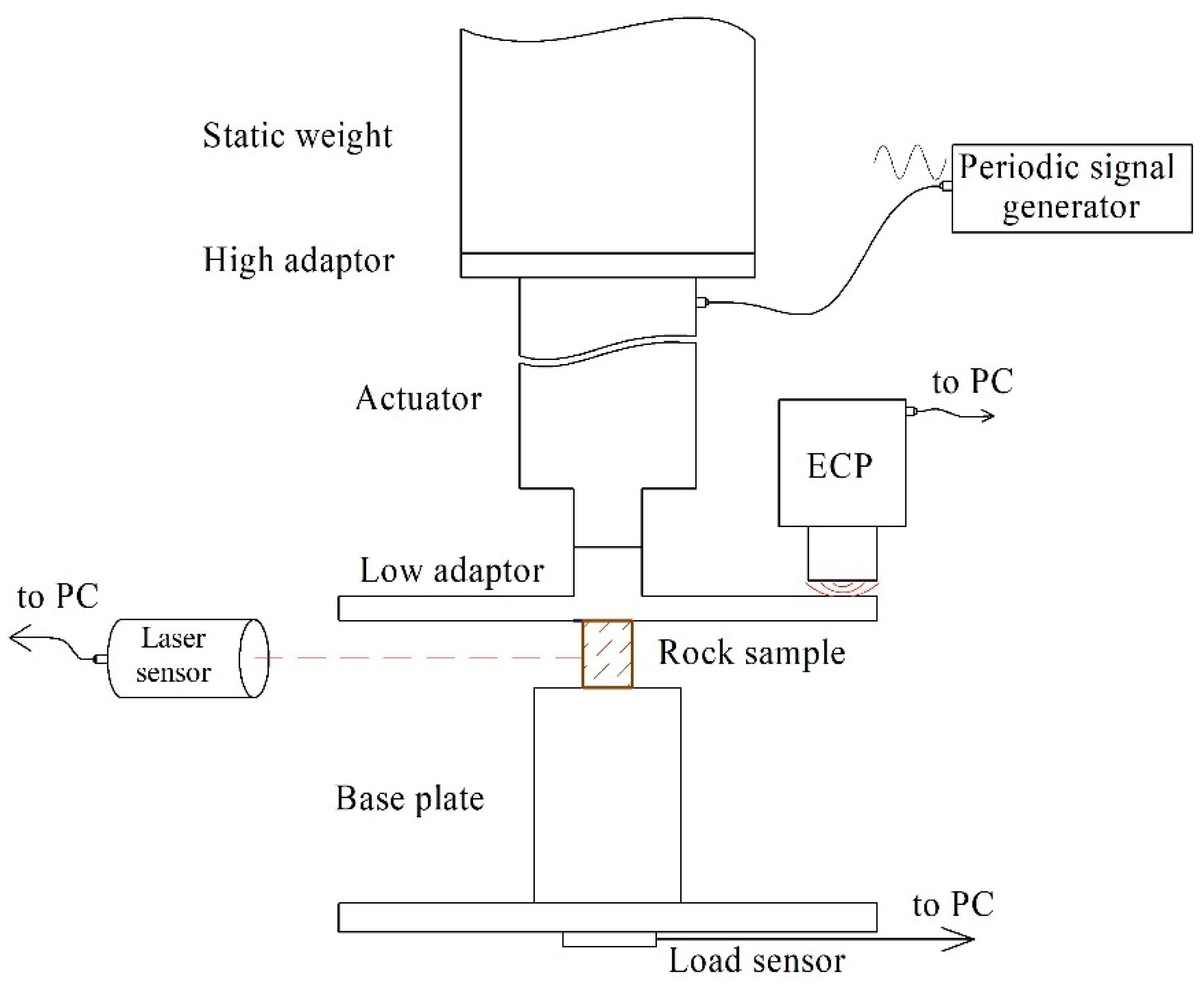
Abstract
1. Introduction
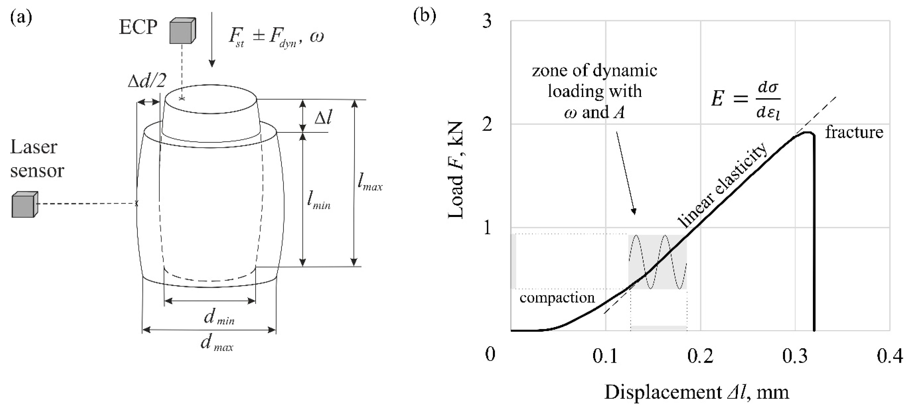
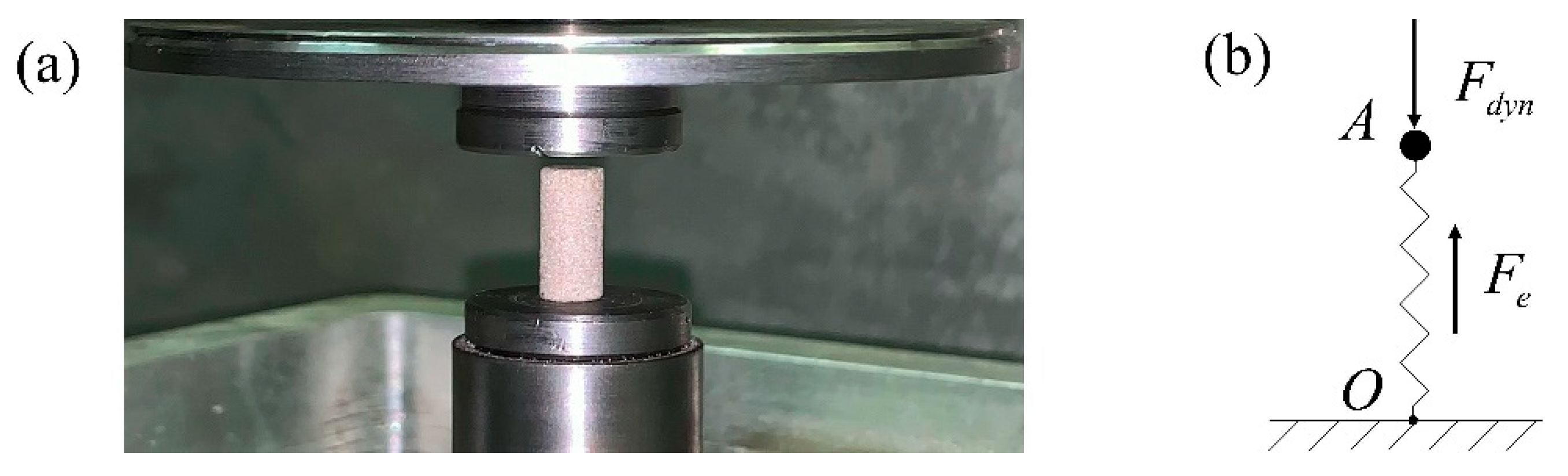
2. Description of the Experiment
3. Model Formulation
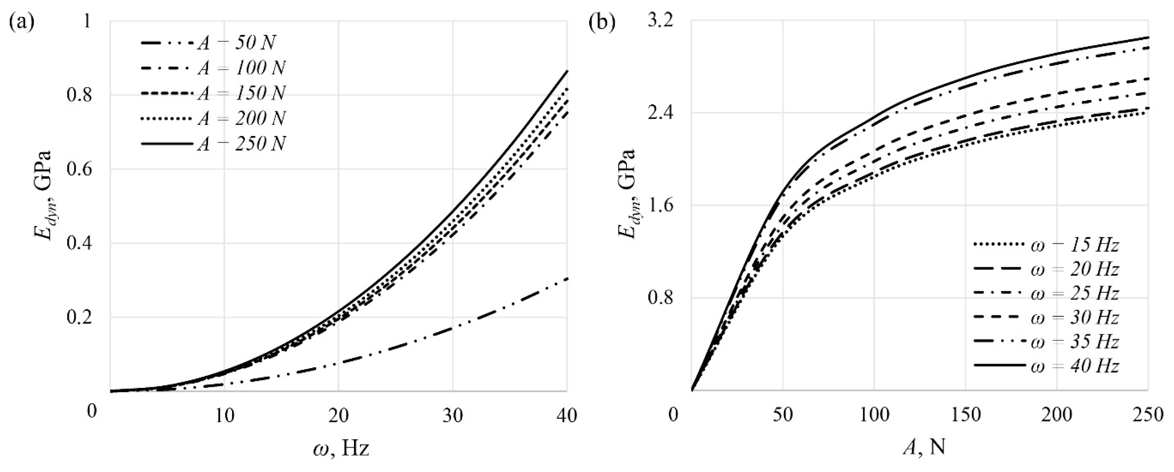
4. Results and Discussion
5. Conclusions
Author Contributions
Funding
Conflicts of Interest
List of Symbols
| A | Amplitude of the dynamic load, N |
| dmax | Maximum value of sample’s diameter, m |
| dmin | Minimum value of sample’s diameter, m |
| Edyn calc | Calculated dynamic component of the Young’s modulus, Pa |
| Edyn model | Model dynamic component of the Young’s modulus, Pa |
| Edyn | Dynamic component of the Young’s modulus, Pa |
| Fst | Static preload, N |
| g | Gravity, m/s2 |
| k | Stiffness |
| l | Sample length, m |
| l0 | Sample length in the preloaded state, m |
| lmax | Maximum sample length, m |
| lmin | Minimum sample length, m |
| m | Mass, m |
| R | Percentage deviation |
| S | Cross-section area of the sample, m2 |
| T | Period, s |
| t | Time, s |
| u | Displacement, m |
| umax | Maximum displacement, m |
| umin | Minimum displacement, m |
| α | Coefficient linking external and natural frequencies |
| Δd | Transverse displacement, m |
| Δl | Longitudinal displacements, m |
| εl | Longitudinal strain |
| π | Ratio of a circle’s circumference to its diameter |
| σ | Stress, Pa |
| ω | External frequency, Hz |
| Ω | Natural frequency, Hz |
References
- Muir, T.G.; Cormack, J.M.; Slack, C.M.; Hamilton, M.F. Elastic softening of sandstone due to a wideband acoustic pulse. J. Acoust. Soc. Am. 2020, 147, 1006–1014. [Google Scholar] [CrossRef] [PubMed]
- Peng, K.; Zhou, J.; Zou, Q.; Song, X. Effect of loading frequency on the deformation behaviours of sandstones subjected to cyclic loads and its underlying mechanism. Int. J. Fatigue 2020, 131, 105349. [Google Scholar] [CrossRef]
- Rivière, J.; Shokouhi, P.; Guyer, R.A.; Johnson, P.A. A set of measures for the systematic classification of the nonlinear elastic behavior of disparate rocks. J. Geophys. Res. Solid Earth 2015, 120, 1587–1604. [Google Scholar] [CrossRef]
- Lozovyi, S.; Bauer, A. Static and dynamic stiffness measurements with Opalinus Clay. Geophys. Prospect. 2019, 67, 997–1019. [Google Scholar] [CrossRef]
- Yin, S.; Xie, R. Experimental analysis of dynamic and static mechanical properties of deep thick anhydrite cap rocks under high-stress conditions. Carbonates Evaporites 2018, 34, 807–823. [Google Scholar] [CrossRef]
- Sone, H.; Zoback, M.D. Mechanical properties of shale-gas reservoir rocks—Part 1: Static and dynamic elastic properties and anisotropy. Geophysics 2013, 78, D381–D392. [Google Scholar] [CrossRef]
- Wang, Y.; Zhao, L.; Han, D.-H.; Qin, X.; Ren, J.; Wei, Q. Micro-mechanical analysis of the effects of stress cycles on the dynamic and static mechanical properties of sandstone. Int. J. Rock Mech. Min. Sci. 2020, 134, 104431. [Google Scholar] [CrossRef]
- Petrie, E.S.; Jeppson, T.N.; Evans, J.P. Predicting rock strength variability across stratigraphic interfaces in caprock lithologies at depth: Correlation between outcrop and subsurface. Environ. Geosci. 2012, 19, 125–142. [Google Scholar] [CrossRef]
- Nazari Ostad, M.; Niri, M.E.; Darjani, M. 3D modeling of geomechanical elastic properties in a carbonate-sandstone reservoir: A comparative study of geostatistical co-simulation methods. J. Geophys. Eng. 2018, 15, 1419–1431. [Google Scholar] [CrossRef]
- Zuo, J.-P.; Wei, X.; Shi, Y.; Liu, C.; Li, M.; Wong, R.H.C. Experimental study of the ultrasonic and mechanical properties of a naturally fractured limestone. Int. J. Rock Mech. Min. Sci. 2020, 125, 104162. [Google Scholar] [CrossRef]
- Li, X.B.; Lok, T.S.; Zhao, J. Dynamic characteristics of granite subjected to intermediate loading rate. Rock Mech. Rock Eng. 2005, 38, 21–39. [Google Scholar] [CrossRef]
- Szewczyk, D.; Bauer, A.; Holt, R.M. A new laboratory apparatus for the measurement of seismic dispersion under deviatoric stress conditions. Geophys. Prospect. 2016, 64, 789–798. [Google Scholar] [CrossRef]
- Szewczyk, D.; Holt, R.M.; Bauer, A. The impact of saturation on seismic dispersion in shales—laboratory measurements. Geophysics 2018, 83, 15–34. [Google Scholar] [CrossRef]
- Batzle, M.L.; Han, D.-H.; Hofmann, R. Fluid mobility and frequency-dependent seismic velocity—Direct measurements. Geophysics 2006, 71, N1–N9. [Google Scholar] [CrossRef]
- Pimienta, L.; Fortin, J.; Guéguen, Y. Bulk modulus dispersion and attenuation in sandstones. Geophysics 2015, 80, A25–A30. [Google Scholar] [CrossRef]
- Gong, F.; Di, B.; Wei, J.; Ding, P.; Tian, H.; Han, J. A study of the anisotropic static and dynamic elastic properties of transversely isotropic rocks. Geophysics 2019, 84, C281–C293. [Google Scholar] [CrossRef]
- Bagde, M.N.; Petroš, V. Fatigue properties of intact sandstone samples subjected to dynamic uniaxial cyclical loading. Int. J. Rock Mech. Min. Sci. 2005, 42, 237–250. [Google Scholar] [CrossRef]
- Aghaei Araei, A.; Razeghi, H.R.; Ghalandarzadeh, A.; Hashemi Tabatabaei, S. Effects of loading rate and initial stress state on stress-strain behavior of rock fill materials under monotonic and cyclic loading conditions. Sci. Iran. 2012, 19, 1220–1235. [Google Scholar] [CrossRef]
- Zhang, Z.; Wang, T.; Wu, S.; Tang, H.; Xin, P.; Liang, C. Dynamics stress–strain behavior of Tianshui soils. Landslides 2017, 14, 323–335. [Google Scholar] [CrossRef]
- ASTM Standard D3999-91. Standard D3999-91. Standard test methods for the determination of the modulus and damping properties of soils using the cyclic triaxial apparatus. In Annual Book of ASTM Standard; ASTM International: West Conshohocken, PA, USA, 2003. [Google Scholar]
- Riabokon, E.P. Laboratory study on the effect of elastic wave treatment on geomechanical and capillary properties of clastic reservoirs. Neftyanoe Khozyaystvo—Oil Ind. 2020, 4, 54–57. [Google Scholar] [CrossRef]
- Wiercigroch, M.; Riabokon, E.P.; Guzev, M.A.; Turbakov, M.S.; Kobiakov, D.V. Experimental studies on static and dynamic loading of heterogeneous rocks. In Proceedings of the XLVIII International Conference Advanced Problems in Mechanics, Saint Petersburg, Russia, 21–26 June 2020; p. 55. [Google Scholar]
- Lomakin, E.V. Mechanics of media with stress-state dependent properties. Phys. Mesomech. 2007, 10, 255–264. [Google Scholar] [CrossRef]
- Myasnikov, V.P.; Sadovskii, V.M. Variational principles of the theory of the limiting equilibrium of media with different strengths. J. Appl. Math. Mech. 2004, 68, 437–446. [Google Scholar] [CrossRef]
- Min, K.-B.; Jing, L. Stress dependent mechanical properties and bounds of Poisson’s ratio for fractured rock masses investigated by a DFN-DEM technique. Int. J. Rock Mech. Min. Sci. 2004, 41, 1–6. [Google Scholar] [CrossRef]
- Makarov, P.V. Evolutionary nature of structure formation in lithospheric material: Universal principle for fractality of solids. Russ. Geol. Geophys. 2007, 48, 558–574. [Google Scholar] [CrossRef]
- Grayeli, R.; Mortazavi, A. Discontinuous deformation analysis with second-order finite element meshed block. Int. J. Numer. Anal. Methods Geomech. 2006, 30, 1545–1561. [Google Scholar] [CrossRef]
- Sadovskii, V.M.; Sadovskaya, O.V. Supercomputer modeling of wave propagation in blocky media accounting fractures of interlayers. Adv. Struct. Mater. 2020, 122, 379–398. [Google Scholar] [CrossRef]
- Liu, G.-Y.; Xu, W.-J.; Govender, N.; Wilke, D.N. A cohesive fracture model for discrete element method based on polyhedral blocks. Powder Technol. 2020, 359, 190–204. [Google Scholar] [CrossRef]
- Chanyshev, A.I.; Belousova, O.E. A method to describe hierarchical block structure of rock mass, considering nonuniformity of mechanical properties. J. Min. Sci. 2017, 53, 441–448. [Google Scholar] [CrossRef]
- Wang, W.; Chen, S. 3D elasto-visco-plastic hierarchical block element method for rock mass. Yanshilixue Yu Gongcheng Xuebao/Chin. J. Rock Mech. Eng. 2003, 22, 525–531. [Google Scholar]
- Li, J.; Chen, W.; Shi, C.; Wang, M. Calculation method of irreversible displacement region radius based on block hierarchical structure under large-scale underground explosion. Baozha Yu Chongji/Explos. Shock Waves 2018, 38, 1271–1277. [Google Scholar] [CrossRef]
- Oparin, V.N.; Tanaino, A.S. Canonical ranking of sizes of structural units in rocks classifications. J. Min. Sci. 2009, 45, 551–562. [Google Scholar] [CrossRef]
- Nikafshan Rad, H.; Jalali, Z.; Jalalifar, H. Prediction of rock mass rating system based on continuous functions using Chaos-ANFIS model. Int. J. Rock Mech. Min. Sci. 2015, 73, 1–9. [Google Scholar] [CrossRef]
- Müller, L. Rock Mechanics; Springer: Wien, Austria; New York, NY, USA, 1982. [Google Scholar]
- Brocato, M. A continuum model of close packing granular materials for the study of rock filled gabions. Int. J. Solids Struct. 2020, 187, 38–47. [Google Scholar] [CrossRef]
- Biot, M.A. Theory of propagation of elastic waves in a fluid-saturated porous solid II. Higher frequency range. J. Acoust. Soc. Am. 1956, 28, 179–191. [Google Scholar] [CrossRef]
- O’Connell, R.J.; Budiansky, B. Viscoelastic properties of fluid-saturated cracked solids. J. Geophys. Res. 1977, 82, 5719–5735. [Google Scholar] [CrossRef]
- Mavko, G.; Nur, A. Melt squirt in the asthenosphere. J. Geophys. Res. 1975, 80, 1444–1448. [Google Scholar] [CrossRef]
- Murphy, W.F., III; Winkler, K.W.; Kleinberg, R.L. Acoustic relaxation in sedimentary rocks: Dependence on grain contacts and fluid saturation. Geophysics 1986, 51, 757–766. [Google Scholar] [CrossRef]
- Johnston, D.H.; Toksoz, M.N.; Timur, A. Attenuation of seismic waves in dry and saturated rocks—II. Mechanisms. Geophysics 1979, 44, 691–711. [Google Scholar] [CrossRef]
- Endres, A.L.; Knight, R.J. Incorporating pore geometry and fluid pressure communication into modeling the elastic behavior of porous rocks. Geophysics 1997, 62, 106–115. [Google Scholar] [CrossRef]
- Dvorkin, J.; Nur, A. Dynamic poroelasticity: A unified model with the squirt and the Biot mechanisms. Geophysics 1993, 58, 524–533. [Google Scholar] [CrossRef]
- Pride, S.R.; Berryman, J.G. Linear dynamics of double-porosity dual-permeability materials. I. Governing equations and acoustic attenuation. Phys. Rev. E Stat. Nonlinear Soft Matter Phys. 2003, 68, 366031–3660310. [Google Scholar] [CrossRef] [PubMed]
- Chapman, M.; Zatsepin, S.V.; Crampin, S. Derivation of a microstructural poroelastic model. Geophys. J. Int. 2002, 151, 427–451. [Google Scholar] [CrossRef]
- Mikhaltsevitch, V.; Lebedev, M.; Gurevich, B. A laboratory study of the elastic and anelastic properties of the sandstone flooded with supercritical CO2 at seismic frequencies. Energy Procedia 2014, 63, 4289–4296. [Google Scholar] [CrossRef]
- Spencer, J.W., Jr. Stress relaxations at low frequencies in fluid-saturated rocks: Attenuation and modulus dispersion. J. Geophys. Res. 1981, 86, 1803–1812. [Google Scholar] [CrossRef]
- Winkler, K.W. Frequency dependent ultrasonic properties of high-porosity sandstones. J. Geophys. Res. 1983, 88, 9493–9499. [Google Scholar] [CrossRef]
- Zhang, Q.B.; Zhao, J. A review of dynamic experimental techniques and mechanical behaviour of rock materials. Rock Mech. Rock Eng. 2014, 47, 1411–1478. [Google Scholar] [CrossRef]
- Ožbolt, J.; Sharma, A.; Reinhardt, H.-W. Dynamic fracture of concrete—Compact tension specimen. Int. J. Solids Struct. 2011, 48, 1534–1543. [Google Scholar] [CrossRef]
- Bažant, Z.P.; Shang-Ping, B.; Ravindra, G. Fracture of rock: Effect of loading rate. Eng. Fract. Mech. 1993, 45, 393–398. [Google Scholar] [CrossRef]
- Tutuncu, A.N.; Podio, A.L.; Gregory, A.R.; Sharma, M.M. Nonlinear viscoelastic behavior of sedimentary rocks, Part I: Effect of frequency and strain amplitude. Geophysics 1998, 63, 184–194. [Google Scholar] [CrossRef]
- Saksala, T. On the strain rate sensitivity of coarse-grained rock: A mesoscopic numerical study. Rock Mech. Rock Eng. 2019, 52, 3229–3240. [Google Scholar] [CrossRef]
- Denoual, C.; Hild, F. A damage model for the dynamic fragmentation of brittle solids. Comput. Methods Appl. Mech. Eng. 2000, 183, 247–258. [Google Scholar] [CrossRef]
- Jaeger, J.C.; Cook, N.G.W.; Zimmerman, R.W. Laboratory testing of rocks. In Fundamentals of Rock Mechanics, 4th ed.; Blackwell Publishing: Malden, MA, USA, 2007; pp. 145–167. [Google Scholar]
- Goldstein, H.; Poole, C., Jr.; Safko, J. Classic Mechanics, 3rd ed.; Addison Wesley: San Francisco, CA, USA, 2002. [Google Scholar]


Publisher’s Note: MDPI stays neutral with regard to jurisdictional claims in published maps and institutional affiliations. |
© 2020 by the authors. Licensee MDPI, Basel, Switzerland. This article is an open access article distributed under the terms and conditions of the Creative Commons Attribution (CC BY) license (http://creativecommons.org/licenses/by/4.0/).
Share and Cite
Guzev, M.; Riabokon, E.; Turbakov, M.; Kozhevnikov, E.; Poplygin, V. Modelling of the Dynamic Young’s Modulus of a Sedimentary Rock Subjected to Nonstationary Loading. Energies 2020, 13, 6461. https://doi.org/10.3390/en13236461
Guzev M, Riabokon E, Turbakov M, Kozhevnikov E, Poplygin V. Modelling of the Dynamic Young’s Modulus of a Sedimentary Rock Subjected to Nonstationary Loading. Energies. 2020; 13(23):6461. https://doi.org/10.3390/en13236461
Chicago/Turabian StyleGuzev, Mikhail, Evgenii Riabokon, Mikhail Turbakov, Evgenii Kozhevnikov, and Vladimir Poplygin. 2020. "Modelling of the Dynamic Young’s Modulus of a Sedimentary Rock Subjected to Nonstationary Loading" Energies 13, no. 23: 6461. https://doi.org/10.3390/en13236461
APA StyleGuzev, M., Riabokon, E., Turbakov, M., Kozhevnikov, E., & Poplygin, V. (2020). Modelling of the Dynamic Young’s Modulus of a Sedimentary Rock Subjected to Nonstationary Loading. Energies, 13(23), 6461. https://doi.org/10.3390/en13236461