X-in-the-Loop Testing of a Thermal Management System Intended for an Electric Vehicle with In-Wheel Motors

Abstract

The article describes an elaboration of the X-in-the-loop (XiL) testing environment for a thermal management system (TMS) intended for the traction electric drive of an electric vehicle, which has each of its wheels driven by an in-wheel motor. The TMS features the individual thermal regulation of each electric drive using a hydraulic layout with parallel pipelines and electrohydraulic pumps embedded into them. The XiL system is intended as a tool for studying and developing the TMS design and controls. It consists of the virtual part and the physical part. The former simulates the vehicle operating in a driving cycle with the heat power dissipated by the electric drive components, which entails the change in their temperature regimes. The physical part includes the TMS itself consisting of a radiator, pipelines, and pumps. The physical part also features devices intended for simulation of the electric drive components in terms of their thermal and hydraulic behaviors, as well as devices that simulate airflow induced by the vehicle motion. Bilateral, real-time interactions are established between the two said parts combining them into a cohesive system, which models the studied electric vehicle and its components. The article gives a description of a laboratory setup, which implements the XiL environment including the mathematical models, hardware devices, as well as the control loops that establish the interaction of those components. An example of using this system in a driving cycle test shows the interaction between its parts and operation of the TMS in conditions simulated in both virtual and physical domains. The results constitute calculated and measured quantities including vehicle speed, operating parameters of the electric drives, coolant and air flow rates, and temperatures of the system components.

1. Introduction

Laboratory testing methods known under the common name of “X-in-the-loop” (where “X” means either a hardware system or its components) constitute a synthesis of physical experiments and virtual simulations [1,2,3,4,5]. This synthesis implies that some part of the studied or elaborated system is presented in a hardware form while the remaining part is virtual. The operating environment of the system can also be either physical or virtual or a combination of these. Bilateral interactions are established between the parts of the system using physical actuation, calculations, and data exchange. Operation of the virtual part should be synchronized (in real time) with the operation of the hardware part. This working principle allows researchers to reconstruct the entire studied system within its operating environment and conduct laboratory tests, which are equivalent to those usually performed at specialized proving grounds under carefully adjusted and/or planned ambient conditions. A further development of this technology is to step beyond the limits of a single laboratory and involve several geographically separated testing facilities holding different components of the studied system, either hardware or virtual, to connect these components and make them operate as a single system [5]. In this case, a real-time synchronization is implemented via network connections (e.g., using the internet) between the computing units of the involved testing facilities.

When geographically extended, the X-in-the-loop technology (hereafter abbreviated as XiL) can be advantageous in studying and developing electric vehicles (EV). It is a state-of-the-art automotive engineering practice that powertrain components of an EV are incorporated into a coordinated chassis control architecture [6]. Specifically, an electric drive is usually integrated into a traction control system, braking system (to provide a regenerative braking feature), and active safety systems such as electronic stability control and torque vectoring [7]. The coordinated control implies a highly coherent interaction between different chassis’ systems and components during the powertrain operation. This interaction is elaborated during the powertrain development process in both virtual and physical domains [8,9,10].

Usually, a vehicle’s powertrain consists of components supplied by several producers and developers. Each of them has its own testing facilities and simulation software optimized specifically for the produced component or system. Often, such facilities are equipped with advanced and unique installations or software that could be unavailable to other developers. To avoid an unnecessary waste of resources and gain maximum benefits from the existing specialized facilities, those facilities can be connected and shared within a XiL environment that consolidates all the developers and researchers involved in the elaboration of an EV. An example of such a XiL environment is currently being built by a European consortium of developers, producers, and researchers [5,11]. The project encompasses all the above-mentioned aspects of the EV integrated chassis development. Its aim is to modify a production EV by introducing a new advanced powertrain, which is based on four in-wheel electric motors having a coordinated control that allows them to deliver traction and regenerative braking functions, as well as functions that improve the vehicle’s drivability and active safety.

One of the aspects regarding the EV integrated chassis development that needs to be covered by the XiL environment is a thermal management system (TMS) of the powertrain. The important role of this system is emphasized by a substantial number of published research including the works [12,13,14,15], which describe the approaches used in designing TMSs for both conventional and electric vehicles. The work presented by this article, being a part of the mentioned joint project, is aimed to elaborate an experimental design of the TMS intended for the considered four-wheel-drive electric vehicle. The main goal of the current stage is to develop a laboratory facility allowing for XiL testing of the TMS, first—autonomously with virtual models substituting the physically absent components and the operating environment (with some simplifications), and then—in cooperation with a remote laboratory having the hardware powertrain with its actual control system.

In the literature, one can find numerous examples of using the X-in-the-loop technology for the research and development of automotive TMSs. In particular, the works [16,17] describe a laboratory setup developed by the National Renewable Energy Laboratory (USA) for XiL tests of thermal management systems intended for electric vehicles. It implements a physical simulation of powertrain components, as well as climatic conditions within the vehicle’s passenger compartment. The simulators of powertrain components contain electric heaters through which the cooling fluid flows. The control of the simulators is provided by thermal mathematical models of the powertrain components operating in real-time synchronously with the hardware part of the setup.

An example of involving the XiL technology in studying the thermal management of the vehicle inner space is shown in [18]. The virtual part of the described system simulates the passenger compartment in terms of its temperature dynamics and its interaction with the surroundings. The physical part includes the tested thermal management system (being a climate-control system) and simulating devices providing its interaction with virtual models of the vehicle’s inner space and the outside environment.

The publications [19,20] describe an elaboration of a physical simulation device intended for XiL testing of automotive thermal management systems designed for electrified powertrains. The device modulates the coolant temperature and flow in accordance with the operating regimes of the tested powertrain or its components. In addition, the device works as an interface between the physical and virtual parts of the tested systems. The device is controlled using both conventional techniques (i.e., PID regulators) and advanced methods including model predictive control. The work [20] demonstrates the performance of this tool in XiL experiments involving a hybrid electric vehicle equipped with a system regenerating the heat energy of an internal combustion engine.

One can also find examples of using the XiL technology in the research of refrigeration thermal management. The work [21] describes such research considering an articulated vehicle equipped with a refrigeration unit. It is noted that the conventional way to test such units implies placing an isothermal trailer (or a semi-trailer) equipped with a refrigeration system inside a climatic chamber replicating ambient conditions. Due to considerable sizes of such trailers, this approach requires large and expensive testing facilities consuming substantial amounts of energy during tests. As an alternative, the work [21] proposes a XiL system, which only implies the physical testing of a refrigeration unit connected to a simulating device. The latter creates an airflow having the specified temperature and speed and conveys this airflow through the output duct into the refrigeration unit. The input duct of the simulating device is connected to the output of the refrigeration unit and receives the cooled air. The temperature of the air to be fed into the tested unit is calculated by a virtual model, which simulates the thermally regulated container and its operating environment.

Analysis of the literature [16,17,18,19,20,21] shows that, in the XiL environments intended for testing of the automotive thermal management systems, the physical part includes the thermal management system itself while the virtual part simulates the powertrain components to be thermally regulated, as well as their operating conditions including ambient factors. There are two types of interaction between these parts of the system: Physical and information. The first type is implemented by a device that physically simulates thermal and hydraulic behaviors of the modeled powertrain’s component, i.e., the coolant pressure drop and the temperature dynamics that would take place in the actual component in the specified operating conditions. The information interaction is implemented by feedback and control signals. The feedback is provided by sensor measurements. The main measured variables are the coolant flow rate, pressure, and temperature at the inlet of the physical simulator. These parameters are relayed into the model of the powertrain component whose output variables are transformed into the command signals for the physical simulator, therefore closing the simulation loop. Models of the powertrain components employed within XiL environments usually consist of lumped parameter dynamic systems implemented by ordinary differential equations. Models of this type do not impose an excessive calculating burden upon the computing devices of the XiL system. This allows for real-time simulations with acceptable accuracy of modeling.

Considering the above principles and the specifics of the TMS designed in this work, the XiL architecture was elaborated. The resulting system and its operation are described in the sequel of the article, which is organized as follows. The next section presents the architecture of the TMS. It is followed by sections describing the concept and implementation of the XiL system and its main parts—physical and virtual. These descriptions are followed by a demonstration of a XiL test that replicates vehicle operation in a driving cycle. The final section gives concluding remarks and outlines research and development tasks to be solved in the sequel of this work.

2. Thermal Management System

The article focuses on the thermal management system of the traction electric drives. The TMS of the traction battery is not included in the scope of the described work based on the following considerations. A traction battery needs to have a temperature regime that differs significantly from that of the electric drive. The optimal temperature window of a lithium-ion battery is narrow, ranging from 15 to 25 °C. This ensures the retention of the battery’s maximum capacity and prevents it from accelerated ageing [22,23]. Matching the traction drive thermal conditions to those of the battery will entail an additional power consumption. For example, an input fluid temperature of 45 °C is normal for an electric drive. No additional power consumption is required to lower the temperature. However, when it comes to a battery, this temperature is far above the optimum window and causes accelerated ageing. Therefore, an additional power would be required to lower the temperature of the entire system. The amount of this power is substantial due to the number of components whose heat dissipation causes the temperature to rise. These considerations suggest that providing the battery with a dedicated thermal management circuit is preferable over incorporating it into a shared circuit along with other electric components. One can find such a solution in, for example, the Chevrolet Volt [24]. The battery’s thermal management circuit should be equipped with its own low-temperature heat exchanger, as well as a heater and a cooler providing the required temperature window. These tasks have been addressed in previous works of the institution represented by the authors [25,26]. The next stage of the described project supposes combining the TMS of the traction electric drive and the TMS of the battery into a single system.

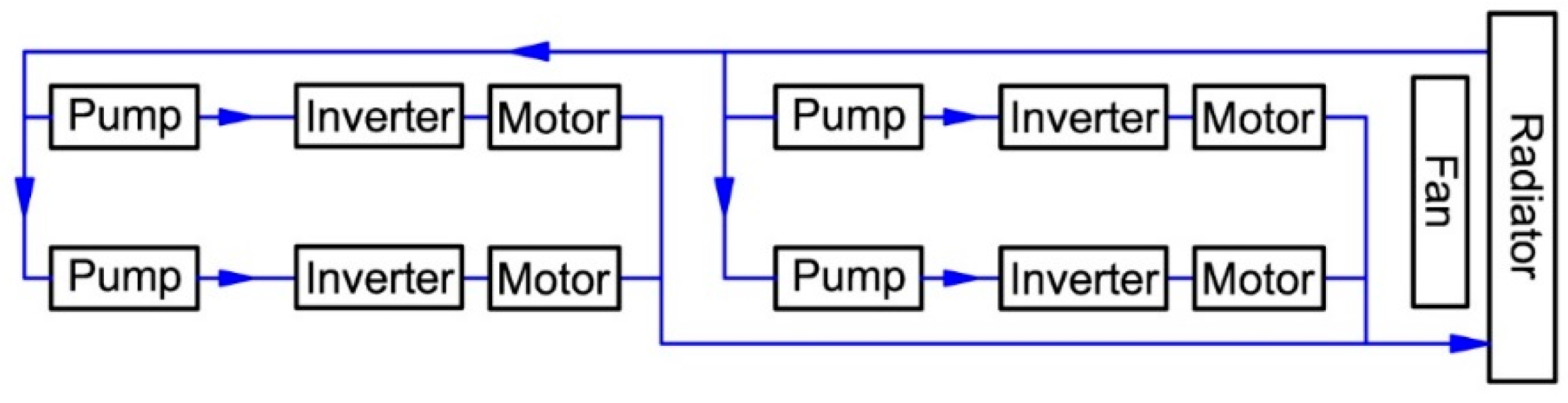
The concept of the TMS intended for the traction electric drive stems from the powertrain architecture that features four electric drives, each associated with an individual wheel. As the control of the powertrain includes functions that regulate torque at each wheel independently, it is advantageous to provide an individual thermal regulation for the electric drives. In order to do this, a dedicated hydraulic circuit is associated with each electric drive. Thus, the TMS includes four circuits that are incorporated into the common hydraulic architecture. The article [27] describes numerical research of several TMS layout options considered in the project. The results of the research suggest two layouts as possible solutions for implementation within the XiL system. Both layouts feature four electrohydraulic pumps located in pipelines (branches), which are parallel to each other. The common suction and supply lines are connected to the branches and to the radiator. The layouts differ in respect of electric drive components embedded into the branches and hydraulic connections between these components. The first layout implies “inverter-motor” pairs with a series interconnection to be embedded into each branch, taking into account their association with the vehicle’s wheels. The second layout features “inverter-inverter” and “motor-motor” pairs with a parallel interconnection embedded into the branches in accordance with their belonging to the front and rear axles. The two layouts have shown approximately the same level of the electrical power consumed by the pumps with a minor advantage of the second layout due to optimized hydraulic resistances of the branches. The further study has also shown that both options provide the same level of thermal performance in a wide range of operating conditions. However, the second layout is more complicated in terms of design, as it requires that pipelines connect the electric drive components situated at opposite sides of the vehicle. The performed comparison allowed the conclusion that the most balanced combination of temperature performance, design aspects, and energy efficiency is provided by the first layout. Thus, it has been selected for implementation within the XiL system. Figure 1 presents a simplified schematic of this layout, omitting the embedded sensors (they are described in Section 3.3) and the expansion hydraulic circuit.

3. X-in-the-Loop System

The virtual subsystem of the XiL setup includes the traction electric drives modeled in aspects of their mechanical performance (i.e., a torque exerted under a given rpm), heat power dissipation, and thermal dynamics. The virtual subsystem also includes the vehicle itself in an aspect of its motion through a predetermined velocity pattern. A control system responding to the driver’s torque request and distributing the requested torque between the front and the rear axles is also provided as a part of the model (see the details in Section 3.2.1).

The main part of the physical subsystem is the TMS itself. The traction electric drive components are physically represented by the simulators—devices that maintain the output coolant temperature and exert the hydraulic resistance corresponding to those of the actual components operating in conditions modeled by the virtual subsystem. The effect of the vehicle motion is physically simulated by an airflow passing through the radiator and supplied by an array of fans placed in front of it. Rotation of the fans is controlled in accordance with the simulated driving conditions.

The XiL system design offers two options that can be used for simulation of the vehicle and its powertrain components, which are not physically presented in the TMS test bench. The option that can be called “local” implies using virtual models of both the vehicle and the powertrain operating in real-time within a computing device directly connected to the test bench. The second option can be called “remote,” as it implies receiving the information on the vehicle and powertrain operation from a testing facility located elsewhere. That facility can also use virtual models or, alternatively, can have its own X-in-the-loop installation with, for example, hardware powertrain components and a software vehicle model. In that case, two XiL systems interact via a network connection. At the stage of the project presented by this article, the “local” option of the virtual subsystem was employed using the models described in Section 3.2.

3.1. Physical Subsystem

Figure 2 shows the physical (hardware) part of the XiL system. The TMS is represented by the radiator and its fan (1), the pipelines (2), four electrohydraulic pumps (3), and the expansion tank (4). The components 5–7 provide physical simulation of the internal and external factors that define operating regimes of the TMS. The thermal simulators of the motors and inverters (5) produce the heat corresponding to that of the modeled components in specified operating conditions. Each simulator constitutes a metallic casing that houses a number of rod-shaped electric heaters arranged as a polar array. A coolant pipe is placed inside the array. The emitted heat is conveyed to the coolant through the thin walls of the pipe. The power electronics housed within the casing (6) control the electrical current of each individual heater by means of pulse-width modulation (PWM). The array of fans (7) simulates the incoming airflow. The casing (8) contains the control and commutation module, which implements low-level control algorithms, receives signals from the sensors and relays them to the top-level control, and also executes commands transmitted from the top-level control. The latter is implemented in a laptop computer; it contains the control systems of the test bench and the TMS, as well as the virtual part of the XiL system and a graphical user control interface. The assembled test bench has been installed in a climatic chamber (Figure 2b), which provides physical modeling of the required ambient conditions.

The hydraulic resistance of the electric drive components is simulated by valves (not seen in Figure 2) adjusted in accordance with the pressure drop characteristics of these components shown in Figure 3. In the case of the motor, the data points were obtained through laboratory testing. For the inverter, such testing was unavailable and the data points were acquired by computational fluid dynamics (CFD) calculations using a 3D model of the inverter. For both components, the data points were obtained under three temperatures of the coolant entering the cooling jackets, namely, −5 °C, +25 °C, and +65 °C. The dotted lines represent the approximation of the data points by second-order polynomials.

3.2. Virtual Subsystem

3.2.1. Vehicle Dynamics Model

Dedicated motors driving individual wheels allow for the implementation of several driving control features including emulation of inter-axle and cross-axle active differentials and yaw stability control. This work only considers the feature that distributes torques between the front and the rear axles, as this functionality is used continuously (unlike those intended for yaw control, which only operate in intensive steering maneuvers) and therefore influences the operation of the thermal management system. The traction control implemented within the vehicle model emulates an inter-axle differential by distributing the torque requested by the driver between the front and rear axles proportionally to the speed difference thereof. When both axles have equal speeds, their torque ratio is 1:1. If the wheel slip at one of the axles exceeds that of another axle, the system subtracts the torque from the former and adds it to the latter.

To take into account the modus operandi of the torque distribution control, the model of vehicle dynamics should include the tire adhesion and slip, as well as distribution of the normal forces. As the representative operating regimes for testing TMSs are driving cycles, which usually do not contain lateral motion, it is sufficient for the vehicle model to include only the longitudinal motion. The model of the vehicle’s motion is derived from an equilibrium of the longitudinal projections of the forces acting on the vehicle. The model of wheel rotational dynamics is derived from an equilibrium of the moments acting on the wheel in its rotation plane. The resulting system of equations reads:

$$\{\begin{array}{l}({ℐ}_m+{ℐ}_w)·{\dot{\omega }}_{w,i}={\tau }_{m,i}-F_{x,i}·r_w-M_{f,i}\\ m_v·{\dot{v}}_{v,x}={\displaystyle \sum _{i=1}^4}{F}_{x,i}-F_{air}\end{array}$$

where ${\tau }_m$ and ${ℐ}_m$ are the in-wheel-motor torque and inertia, respectively; ${\omega }_w$ and ${ℐ}_w$ are respectively the wheel angular speed and inertia; $F_x$ is the longitudinal tire force; $r_w$ is the wheel radius; $M_f$ is the tire rolling resistance moment; $m_v$ is the vehicle mass; $v_{v,x}$ is the vehicle longitudinal velocity; $F_{air}$ is the air drag force. Note that the equation of wheel rotational dynamics corresponds to the i-th wheel, where i = 1, …, 4.

The rolling resistance is approximated by a second-order polynomial function of the vehicle speed [28]: $M_f=F_z·\left(f_0+k_v·v_{v,x}^2\right)r_w$, where $F_z$ is the normal force, $f_0$ is the rolling resistance coefficient at near-zero velocity, and $k_v$ is the rolling resistance velocity gain constant. The air drag force is also expressed as a second-order function of the vehicle speed: $F_{air}=0.5·c_x·A_{veh}·{\rho }_{air}\left(T_{air}\right)·v_{v,x}^2$, where $c_x$ is the air drag coefficient, $A_{veh}$ is the area of the vehicle’s frontal projection, and ${\rho }_{air}\left(T_{air}\right)$ is the ambient air density as a function of its temperature.

The distribution of normal forces is calculated using formulae stemming from a static equilibrium of the moments acting on the vehicle in its longitudinal plane. The tire–road adhesion characteristics as a function of the longitudinal slip are approximated using a well-known empirical model called the Magic Formula [29].

Table 1. Parameters for the model of vehicle dynamics.

${\mathit{m}}_{\mathit{v}}\left(\mathbf{kg}\right)$	${\mathit{r}}_{\mathit{w}}\left(\mathbf{m}\right)$	${\mathit{ℐ}}_{\mathit{m}}+{\mathit{ℐ}}_{\mathit{w}}\left(\mathbf{kg}\text{·}{\mathbf{m}}^2\right)$	${\mathit{C}}_{\mathit{x}}$	$\mathit{A}$, (m2)	${\mathit{f}}_0$	${\mathit{k}}_{\mathit{v}}$
3130	0.365	2	0.3	2.65	0.008	4·10−6

contains the main parameters of the vehicle dynamics model that define the power to be produced or consumed by the in-wheel motors while driving, which in turn, defines the power losses dissipated as heat in the electric drives.

3.2.2. Traction Electric Drive Model

The heat power dissipated by the motors and inverters is calculated using the operating parameters and efficiency characteristics of these components:

$$\begin{gathered} P_{heat,m}=\left|P_{m,el}-P_{m,mech}\right|=\left|\frac{{\tau }_m·{\omega }_m}{{\eta }_m^{sgn\left(P_m\right)}}-{\tau }_m·{\omega }_m\right|, \\ {P}_{heat,inv}=\left|P_{inv,el}-P_{m,el}\right|= \left|\frac{P_{m,el}}{{\eta }_{inv}^{sgn\left(P_m\right)}}-P_{m,el}\right|, \end{gathered}$$

where $P_{m,mech}$ and $P_{m,el}$ are the mechanical and electric power of the in-wheel motor, respectively, $P_{inv,el}$ is the electric power at the inverter’s input, ${\eta }_m^{sgn\left(P_m\right)}$ and ${\eta }_{inv}^{sgn\left(P_m\right)}$ are the efficiencies of the motor and inverter, and ${\omega }_m$ is the angular speed of the motor equal to that of the corresponding wheel (${\omega }_w$).

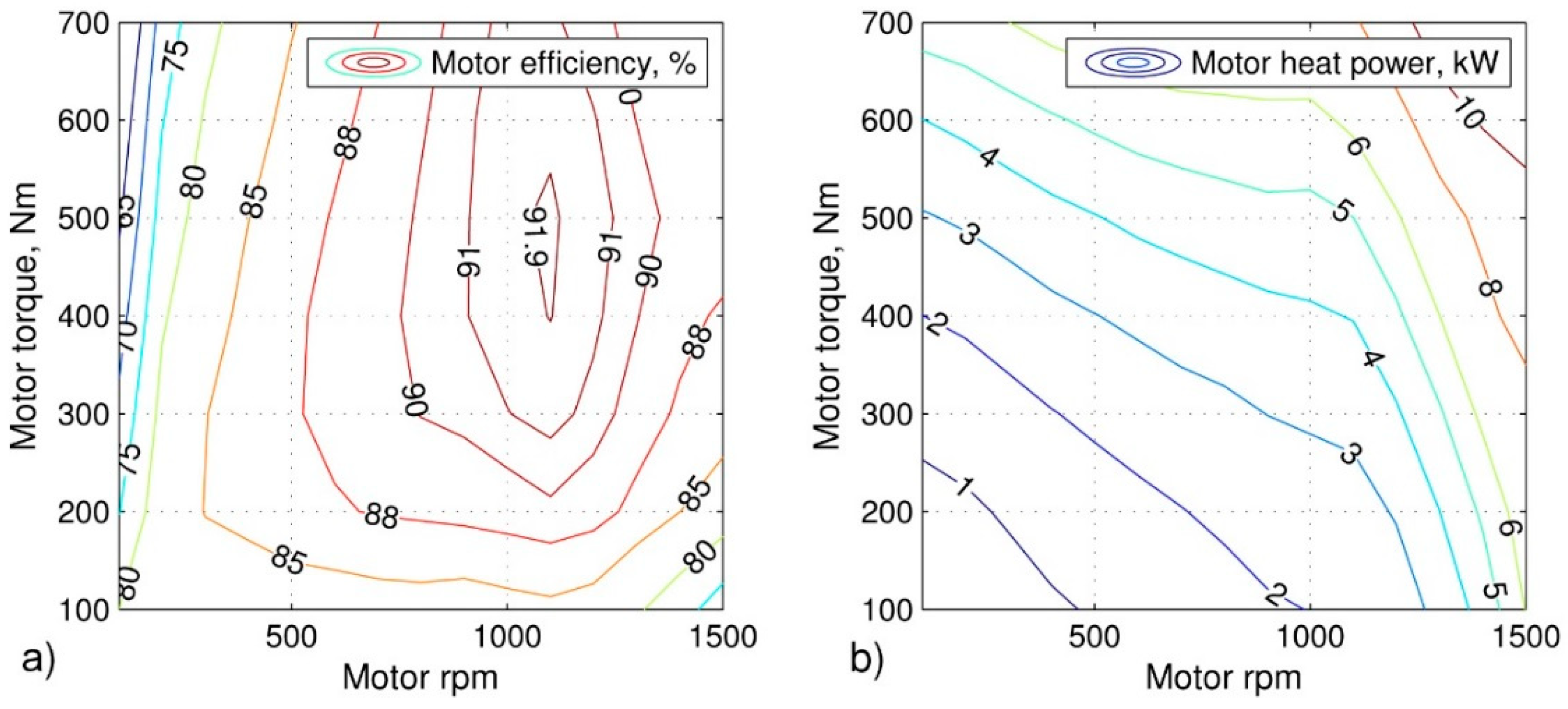
Figure 4 and Figure 5 show the maps of the efficiency and dissipated heat power of the electric motor and the inverter, respectively. The maps were obtained from experimental data provided by the manufacturer of the traction electric drive. The shown ranges of rpm and torque correspond to the continuous mode of the electric drive, beyond which it is not allowed to operate.

In order to simulate temperature behavior of the electric components, a thermal model has been elaborated, which consists of two lumped masses: The fluid flowing within the cooling jacket of the component, and the component’s body. It is assumed that the bulk of the heat transfer between these masses takes place in the form of convection. It has to be taken into account that the actual heat flux is generated within a certain volume (for example, in the stator windings of the motor), which is separated from the coolant flow by a wall whose thickness defines the dynamics of transferring the heat into the coolant. However, a lumped mass model cannot replicate this mechanism—it can only simulate a heat source that affects the lumped mass as a whole. To imitate how remote the heat source from the coolant flow is, the heat power is divided between the lumped masses of the component’s body and the fluid in a proportion defined by weighting factors. The closer the heat source is to the fluid, the larger the corresponding weighting factor and vice versa. Using these assumptions yields the following equations describing a two-mass thermal system:

$$\{\begin{array}{l}\frac{d{\tilde{T}}_{fluid}}{dt}=\frac{c_{fluid}·{\dot{m}}_{fluid}\left(T_{fluid,in}-T_{fluid,out}\right)+k_{heat,fluid}·P_{heat}-{\alpha }_{fluid-body}·A_{fluid-body}\left({\tilde{T}}_{fluid}-{\tilde{T}}_{body}\right)}{c_{fluid}·m_{fluid}}\\ \frac{d{\tilde{T}}_{body}}{dt}=\frac{{\alpha }_{fluid-body}·A_{fluid-body}\left({\tilde{T}}_{fluid}-{\tilde{T}}_{body}\right)+k_{heat,body}·P_{heat}-{\alpha }_{body-air}·A_{body-air}\left({\tilde{T}}_{body}-{\tilde{T}}_{air}\right)}{c_{body}·m_{body}}\end{array}$$

where $\tilde{T}$ is the average temperature of a lumped mass; $T_{\dots ,in}$ and $T_{\dots ,out}$ are the temperatures at the fluid inlet and outlet, respectively; $m_{\dots }$ and $c_{\dots }$ are the mass and the specific thermal capacity of a given lumped object, respectively; ${\alpha }_{\dots -\dots }$ is the coefficient of convective heat transfer between two adjacent lumped masses; $A_{\dots -\dots }$ is the surface conducting the convective heat transfer; $P_{heat}$ is the heat power dissipated within the component; $k_{heat,fluid}$ and $k_{heat,body}$ are the heat power weighting factors assigned to the fluid and the body, respectively. The weighting factors satisfy the following condition: $k_{heat,fluid}+k_{heat,body}=1$.

The heat transfer coefficients were calculated using empirical formulae based on geometry and material properties of the components, as well as the coolant flow regime and temperature [30,31,32].

For a pipeline having an arbitrary shape of the cross-section, the Reynolds number is calculated with the well-known formula:

$$Re=\frac{d_{pipe,eq}·v_{fluid}}{\nu \left(T_{fluid}\right)},$$

where $v_{fluid}$ is the velocity of the fluid flow, $\nu \left(T_{fluid}\right)$ is the kinematic viscosity of the fluid as a function of its temperature, and $d_{eq}$ is the equivalent diameter of the pipeline’s cross-section:

$$d_{pipe,eq}=4A_{\varnothing pipe}/{\mathsf{\Pi }}_{\varnothing pipe},$$

where $A_{\varnothing pipe}$ and ${\mathsf{\Pi }}_{\varnothing pipe}$ are the area and the perimeter of the pipeline’s cross-section, respectively. These parameters, as well as other geometric attributes, were defined from the 3D models of the electric drive components.

The critical values of the Reynolds number corresponding to the threshold between laminar flow and turbulent flow were assumed as 2300 for the fluid and 1000 for the air [31].

The coefficient of convective heat transfer is calculated using the known formula:

$$\alpha =\left(\lambda ·Nu\right)/d_{pipe,eq},$$

where $\lambda$ is the heat conductivity of the cooling medium, and $Nu$ is the Nusselt number calculated using the empirical formulae, taking into account the flow regime of the cooling medium and the geometry of the pipeline.

For the laminar flow of the cooling fluid, the Nusselt number is defined as follows [31]:

$$Nu= k_{Nu-fluid,1}{\left(Re·Pr·d_{pipe,eq}/l_{pipe}\right)}^{1/k_{Nu-fluid,2}},$$

where $Pr$ is the coolant’s Prandtl number being a function of the coolant temperature, $l_{pipe}$ is the length of the pipe, and $k_{Nu-fluid,1}$ and $k_{Nu-fluid,2}$ are empirical coefficients whose approximate values are 1.8 and 3, respectively.

In the case of turbulent coolant flow, the Nusselt number is calculated using Gnielinski–Petukhov’s formula [31,32]:

$$Nu= \frac{\xi }{8}Re·Pr\frac{1}{1+\frac{900}{Re}+12.7\sqrt{ \frac{\xi }{8}}(P{r}^{2/3}-1)},$$

where $\xi$ is the coefficient of friction between the pipe’s wall and the fluid that is defined as follows:

$$\xi ={\left(0.79\ln \left(Re/8\right)\right)}^{-2}.$$

The considered in-wheel motor has a coil-type cooling jacket, which requires using the formula for circular pipelines to calculate the Nusselt number [31]:

$$Nu=N{u}_0\left(1+3.5\frac{d_{pipe,eq}}{2R_{coil}}\right),$$

where $N{u}_0$ is the Nusselt number for the “straightened” coil, which is equivalent to an ordinary straight pipeline calculated using the above formulae. $R_{coil}$ is the radius of the coil.

Additionally, a special equation is used for the Reynolds number when applied to a coil-type pipeline [31]:

$$Re=2·{10}^4{\left(\frac{d_{pipe,eq}}{2R_{coil}}\right)}^{0.32}.$$

For the air flowing along the surfaces of the electric drive components, the Nusselt number reads as follows [31]:

$$Nu= k_{Nu-air,1}R{e}^{k_{Nu-air,2}}P{r}^{k_{Nu-air,3}},$$

where the empirical coefficients $k_{Nu-air,1}$, $k_{Nu-air,2}$, and $k_{Nu-air,3}$ are defined by the flow regime of the air.

3.2.3. Airflow Model

To simulate the airflow passing through the radiator, a map is used that plots this airflow against the vehicle speed. The map (see Figure 6) was derived from an experimental characteristic of an actual heat exchanging system taking into account the equipment placed before the radiator (namely, a condenser). The experimental data have been scaled to match the size of the system that is being designed in this work. Specifically, the original experimental characteristic was downsized, as the prototype radiator system was intended for a larger powertrain.

At the test bench, the airflow induced by the simulating fans is measured by a flow meter (anemometer). However, in the operating regimes when the radiator fan is also enabled, the readings of that sensor will show the combined flow created by two sources (i.e., the radiator fan and the test bench fans). To provide the test bench control system with the correct feedback corresponding to the actual vehicle speed, the airflow created by the radiator’s fan must be subtracted from the total airflow. This requires a map of the combined performance corresponding to the simultaneous operation of both airflow sources with different combinations of their command signals. The map should be derived experimentally—it cannot be calculated by a simple summation of the individual performances, because of mutual influences of the airflows created by the fans during their simultaneous operation. However, the low-level controller of the radiator fan has its own inner algorithms of activation with certain delays and transients, which complicate the estimation of the airflow portion induced by this fan and subtraction of this portion from the combined performance map. As an alternative, during the radiator fan operation, the measured airflow feedback can be replaced by a calculated one corresponding to the sole operation of the test bench fans with a given command signal. The test bench fans activate immediately after receiving a command signal and do not have additional control complications. Therefore, their response is simpler in regard of a mathematical approximation. Thus, it was decided to use this approach to provide the test bench control system with an adequate airflow feedback signal when the radiator fan activates.

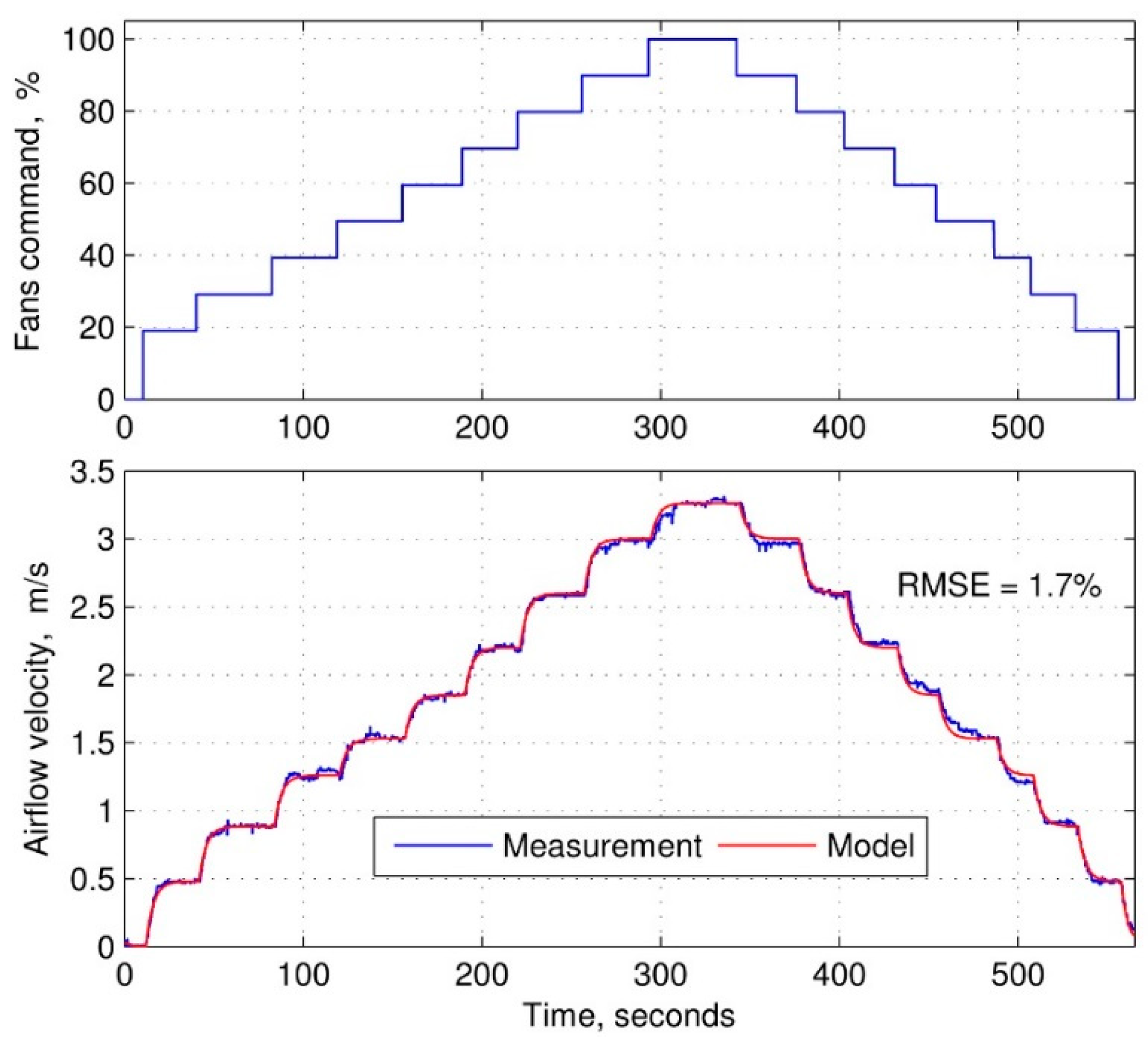
The basic tool for implementing the selected approach is an experimental map of the airflow supplied by the test bench fans when the radiator fan is disabled. In order to obtain that map, the control signal of the test bench fans was regulated in a stepwise manner, beginning with an ascending sequence followed by a descending sequence. After each step, the control signal was kept constant to obtain a steady airflow. The resulting data constitute a static model of the test bench fans’ performance. However, for accurate calculations, a dynamic model is required, which takes into account the response time of the fans, dynamics of the airflow itself, and finally, the dynamic performance of the anemometer. The transient response of the measured airflow to the command signal has shown a pronounced exponential behavior with no significant oscillations. Therefore, the dynamics can be modeled with an acceptable accuracy by a first-order approximation:

$$\frac{d{v}_{air,dyn}}{dt}=\frac{v_{air,stat}\left(u_{fans}\right)-v_{air,dyn}}{{\tau }_{airflow}},$$

where $v_{air,dyn}$ is the air speed calculated by taking into account the system’s dynamics, $v_{air,stat}\left(u_{fans}\right)$ is the air speed calculated using a static map as a function of the command signal, and ${\tau }_{airflow}$ is the time constant considering all the above-mentioned delaying factors.

Figure 7 shows the results of an experiment with a stair-shape control of the bench fans and an approximation of its results by means of the previously obtained static map modified with the above first-order dynamics. One can see that the model provides a good accuracy of airflow calculation. The root-mean-square error (RMSE) of the model amounted to 1.7%, which was considered acceptable.

To verify the airflow model in the conditions for which it was intended, a test was conducted with both the test bench fans and the radiator fan active. The results are shown in Figure 8. From the command signals, one can see that the fans of the test bench simulated constant levels of the external airflow. Meanwhile, the radiator fan created an additional flow, which was increased in a stepwise manner. The total airflow was measured by the anemometer. The model used the command signal of the test bench fans to calculate the portion of the airflow (or velocity) supplied by them.

3.3. Interfacing the Physical and the Virtual Subsystems

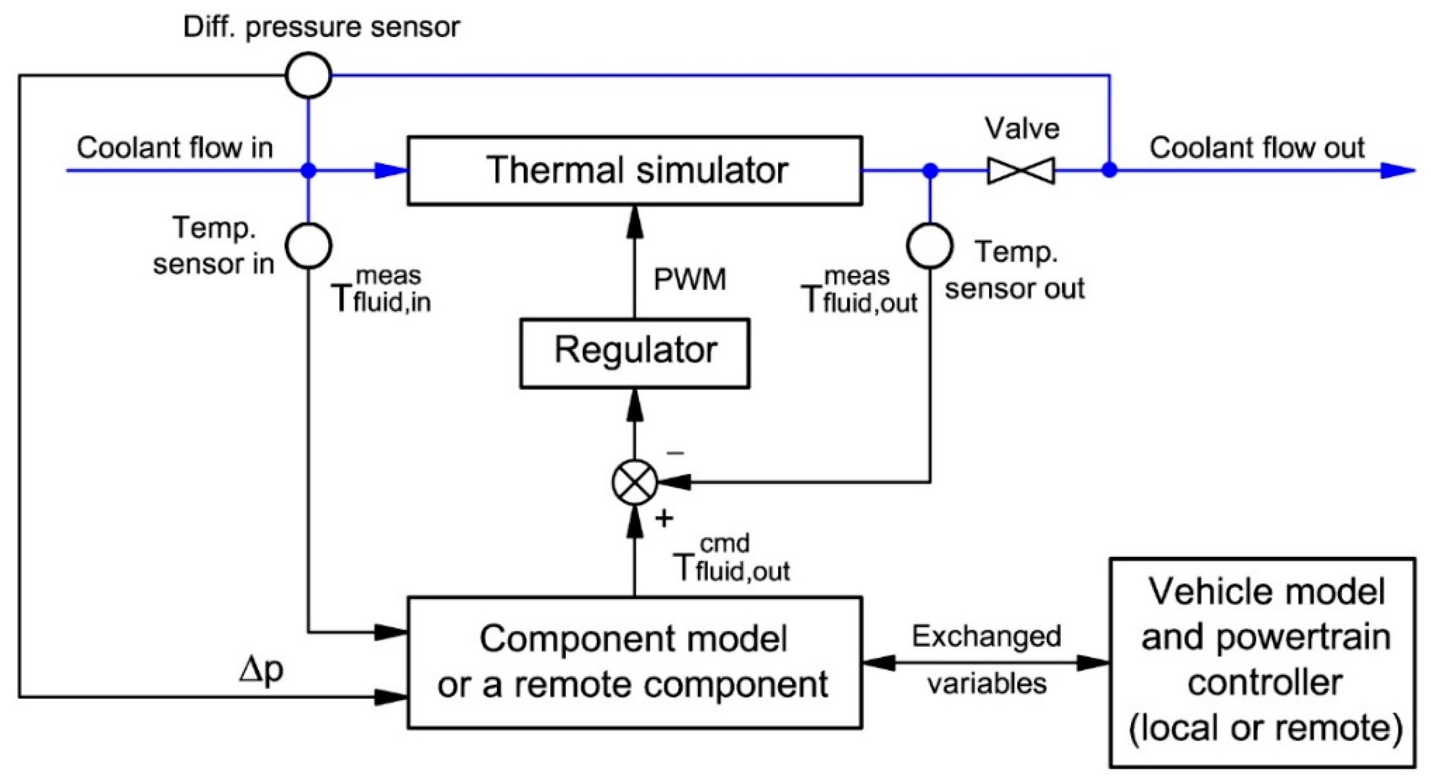
As it was mentioned above, the XiL environment employs physical, information, and control interactions. The most complex simulation loops of the elaborated XiL system are those substituting the components of the electric drive. Figure 9 shows the structure of such a simulating loop including its hardware and software parts (similar arrangements are used for all the simulated electric drive components). The diagram reflects the above-described options that can be employed for simulation of the vehicle and its powertrain components, which are not physically presented in the TMS test bench, namely, the “local” simulation and the “remote” simulation. Most of the elements shown in Figure 9 belong to the control loop intended for the temperature simulation. The thermal model of the electric drive component uses the measured values of the coolant temperature at the component’s inlet, the differential pressure ($\Delta p$) translated into the flow rate, and the ambient air temperature, as well as the calculated value of the heat dissipation defined by the component operating points, to calculate the output coolant temperature. The latter is transferred from the virtual domain into the physical domain by means of the thermal simulator controlled by the regulator. The “Regulator” block contains a proportional-integral (PI) regulator that calculates the PWM duty ratio compensating the deviation between the commanded value of the output temperature (indicated by the “cmd” superscript) and the measured one (provided with the “meas” superscript). The resulting duty ratio is fed into a PWM generator, which converts it into pulses.

The valve simulates the hydraulic resistance expressed as a pressure drop, which is measured by the differential pressure sensor. In addition, in absence of a flow meter (flow meters are not used in the TMS, due to their substantial hydraulic resistance), the differential sensor allows for indirect estimation of the coolant flow rate. This requires preliminary tests to be performed with direct measurements of the flow rate and mapping it against the pressure drop.

Simulation of the incoming airflow is controlled using a simple closed loop, which regulates the operation of the test bench fans. The command signal is the airflow corresponding to the vehicle velocity and calculated using the model described in Section 3.2.3. The feedback signal is either the measured or calculated airflow depending on whether the radiator fan is active or not. The difference between the command and feedback values is compensated using a PI-regulator, which generates a PWM duty ratio signal controlling the test bench fans.

4. X-in-the-Loop Testing Results

The most representative vehicle operating mode to test a thermal management system is a driving cycle conducted in specified ambient conditions. In the preceding numerical study [27], the simulations were performed in two driving cycles, namely, WLTC (World Harmonized Light Vehicles Test Cycle) and ARTEMIS [33]. As the WLTC has been agreed between the project’s participants as a basic schedule, it was used in the XiL tests of the developed TMS. Figure 10 shows an example of testing results obtained in this cycle. The ambient air temperature was being maintained at the +20 °C level. That condition made it sufficient to keep the constant coolant flow rates of 6 L/min in each of the TMS hydraulic branches to keep the coolant temperature at the radiator inlet below +35 °C. Both virtual (calculated) and physical (measured) variables are presented in Figure 10 including the vehicle velocity (Veh. vel.) calculated by the model, the speed of the air passing through the radiator calculated by the model map (see Figure 6) and measured by the anemometer (the radiator fan was inactive in this test; hence, using the model to estimate the airflow feedback was not required), as well as the calculated wheel torques and heat power dissipated by the electric drive components associated with the front and rear axles. The three bottom plots show calculated and measured thermal variables by the examples of one electric motor (the front right unit), one inverter (also the front right unit), and the radiator.

The output coolant temperatures were calculated by the thermal models in response to the measured values of the input coolant temperatures, the coolant flow rates, and the ambient air temperature. The measured output coolant temperatures resulted from the operation of the thermal simulators that tracked the commands calculated by the models. One can see that the simulating devices provided a good tracking quality with a maximum error of ca. 0.5 °C in the case of the motor. For the inverter, the tracking quality was noticeably better due to a substantially lower loss of power than that of the motor and, consequently, lower required power of the heaters. One can compare the heat dissipated by the motor to that of the inverter by examining the coolant temperature differences between the inlets and outlets of these components. For the motor, this difference amounted up to 4.8 °C, while for the inverter, it did not exceed 1.6 °C. The temperature difference between the radiator’s inlet and outlet characterizes the heat energy dissipated into the environment. It reaches the maximum value of ca. 5 °C in the highway part of the driving cycle where the heat is taken away by an intensive airflow created by the test bench fans.

In the graphs, the torques at the front and rear wheels visually coincide. A closer look reveals that differences between them do not exceed 50 Nm, which is explained by the road conditions simulated. The road was assumed level and covered with dry asphalt having a maximum adhesion coefficient of 1. As the accelerations and decelerations in the WLTC are moderate (up to 1.75 m/s²), the tire slip is small and no substantial changes in the normal forces occur, making the torque, which compensates the speed differential of the front and rear wheels, relatively small.

5. Conclusions and Future Work

A thermal management system for a traction electric drive of a four-wheel-drive electric vehicle equipped with in-wheel motors has been designed. The TMS features four electrohydraulic pumps providing individual coolant flow regulation within the cooling jackets of the electric drive components associated with each wheel. The laboratory facility for XiL testing of the TMS has been developed, consisting of the virtual and physical subsystems and providing bilateral interactions of these subsystems involving information exchange and physical actuation. The elaborated thermal simulator and its control loop provide a good quality of tracking the coolant temperature calculated by the thermal models. The inverter thermal simulation is more precise than that of the motor due to the substantially lower heat power dissipated by the former.

The XiL system allows for elaboration of the TMS design and controls with involvement of the actual components (pumps, radiator, fan, pipelines), which makes the elaborated system closer to the one that will be implemented in an actual EV. On the other hand, the XiL system allows for replication of different operating conditions of the TMS with accurate repeatability by means of the mathematical models constituting the virtual part, which makes it a good tool for research work. The simulating loop for an electric drive component described in Section 3.3 is self-containing and, therefore, can be implemented in different arrangements of TMS-XiL systems not limited to the one described in this article. In particular, it can be used in physical simulations of electric drives (featuring either in-wheel or chassis-mounted motors) employed in pure- or hybrid electric vehicles with different configurations of driven wheels. The virtual part of the simulating loop can be either “local” or “remote.” The latter option allows the extension of the XiL system beyond the limits of the laboratory housing the TMS and the interaction (via the Internet) with other facilities containing software or hardware powertrain components or their combinations. In that way, the TMS laboratory can be incorporated into a shared environment for the elaboration and studying of the entire powertrain, overcoming limits of geographical scattering.

In the sequel of the project, the TMS-XiL system is supposed to be connected and synchronized with the remote laboratory that houses the hardware version of the traction electric drive and a software model of the vehicle with a controller that implements such functions as braking torque blending, yaw stability control, and active suspension control. The control system of the TMS, which at the presented stage of the project, has been designed in a simplified way, is to be further elaborated and tested within the XiL environment. Another future task mentioned in Section 2 is combining the thermal management systems of the traction electric drive and the traction battery to provide thermal regulation for the entire powertrain.