Powertrain Optimization for Electric Buses under Optimal Energy-Efficient Driving


Abstract
1. Introduction
2. Methodology
2.1. Vehicle Speed Optimization
2.2. Ride Comfort Evaluation
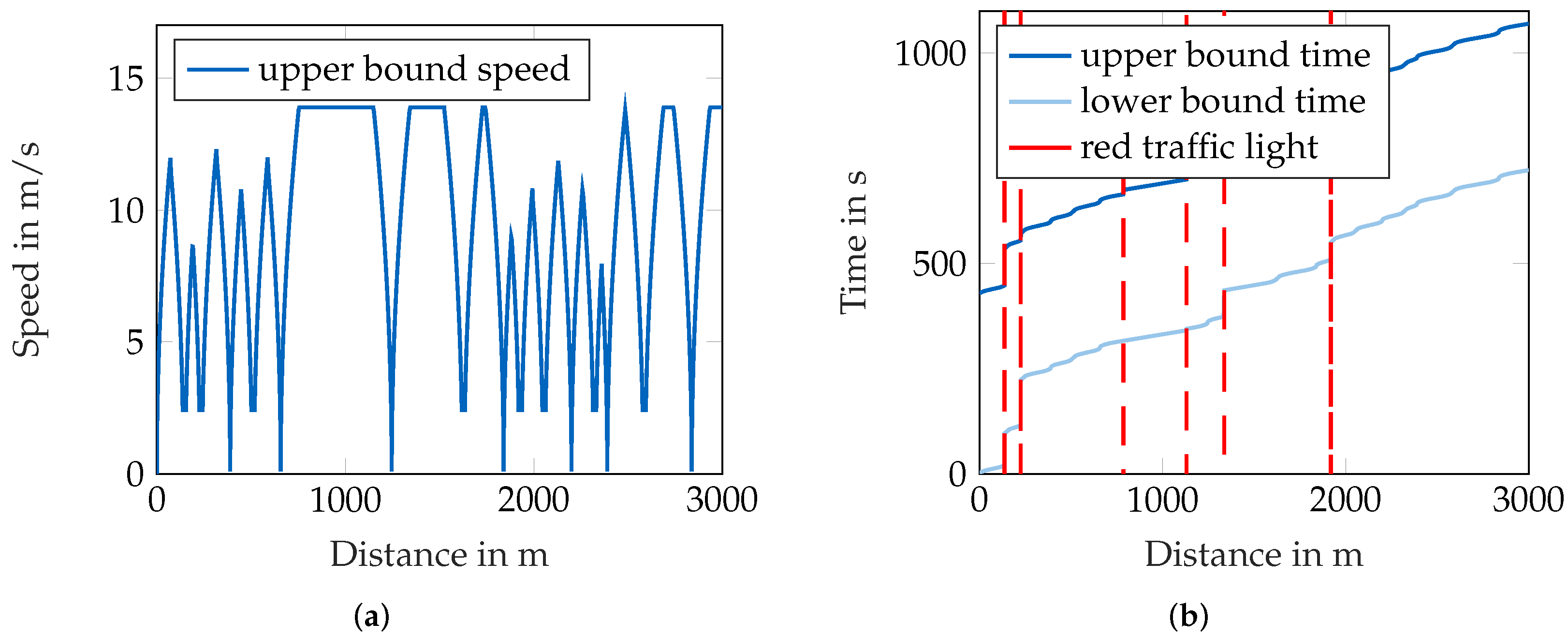
2.3. Derivation of Boundary Conditions and Discretization
2.4. Assumptions
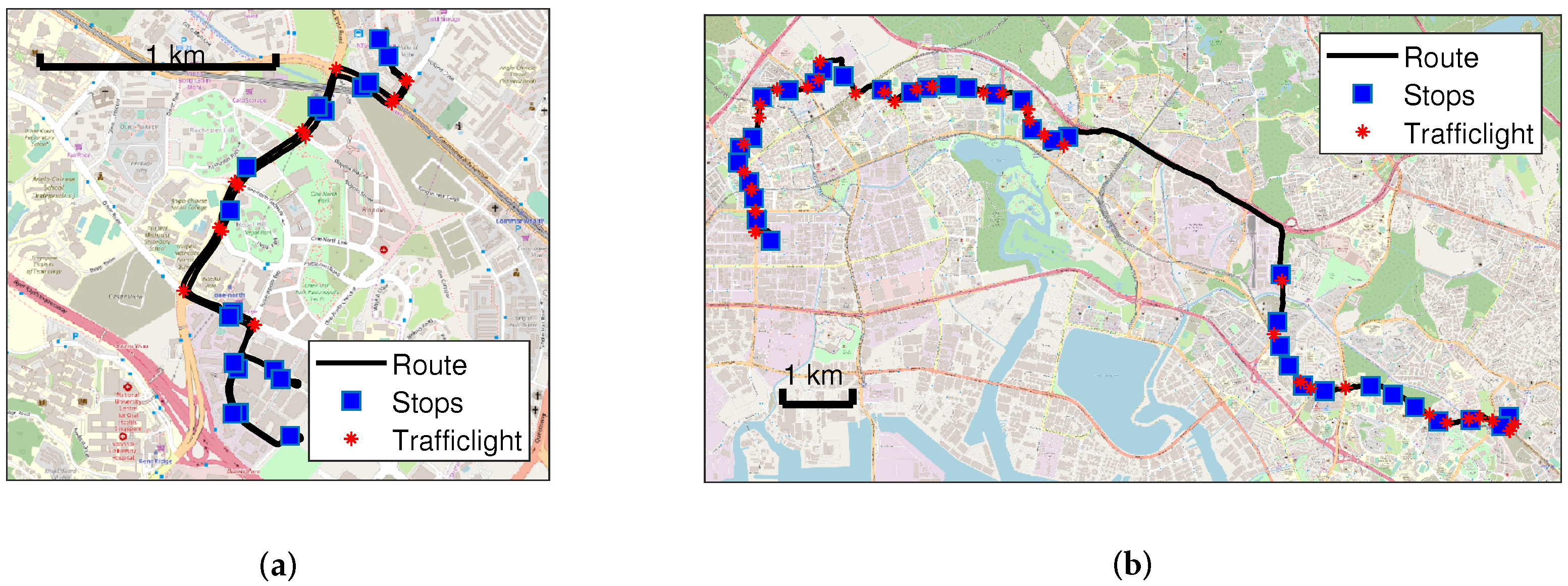
3. Case Study
4. Results
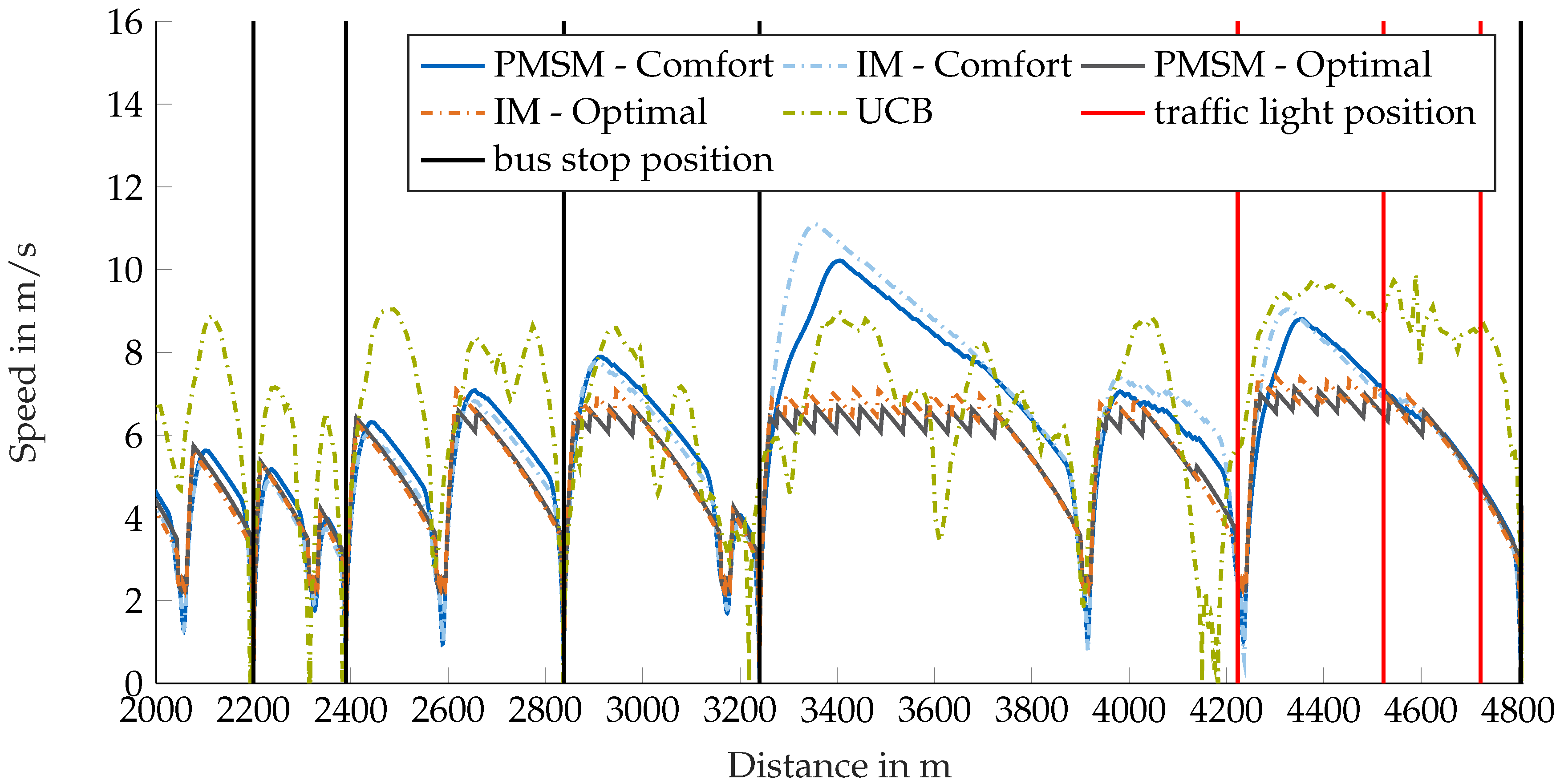
4.1. Speed Profiles
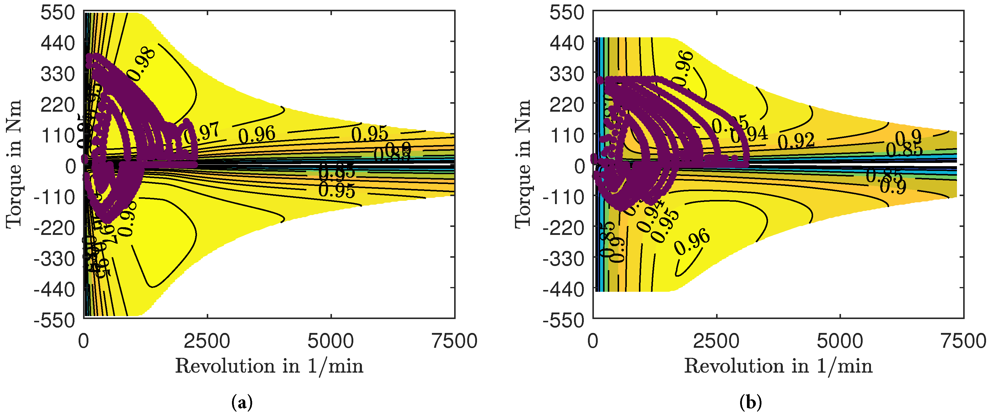
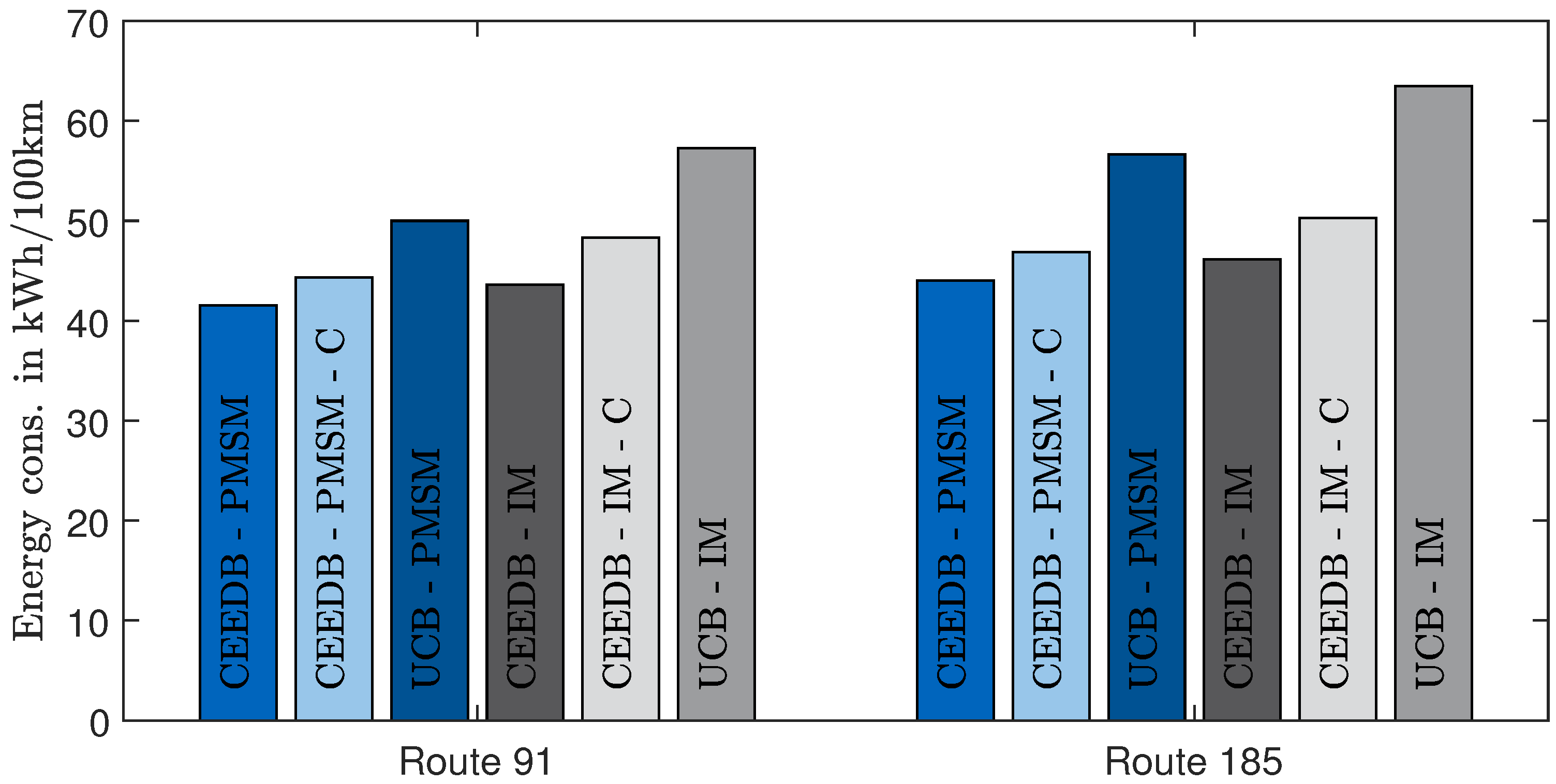
4.2. Powertrain Optimization Analyses
5. Discussion
5.1. Sensitivity Analysis
5.2. Ride Comfort
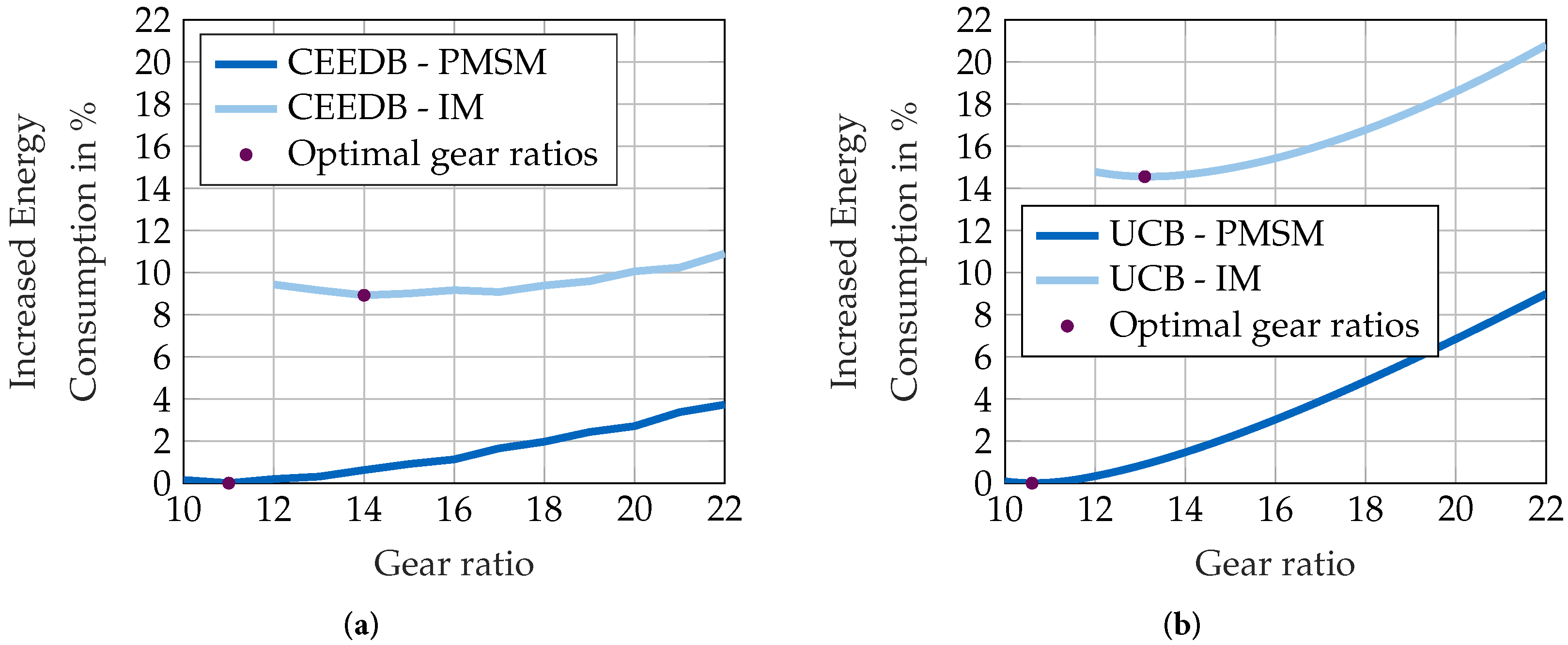
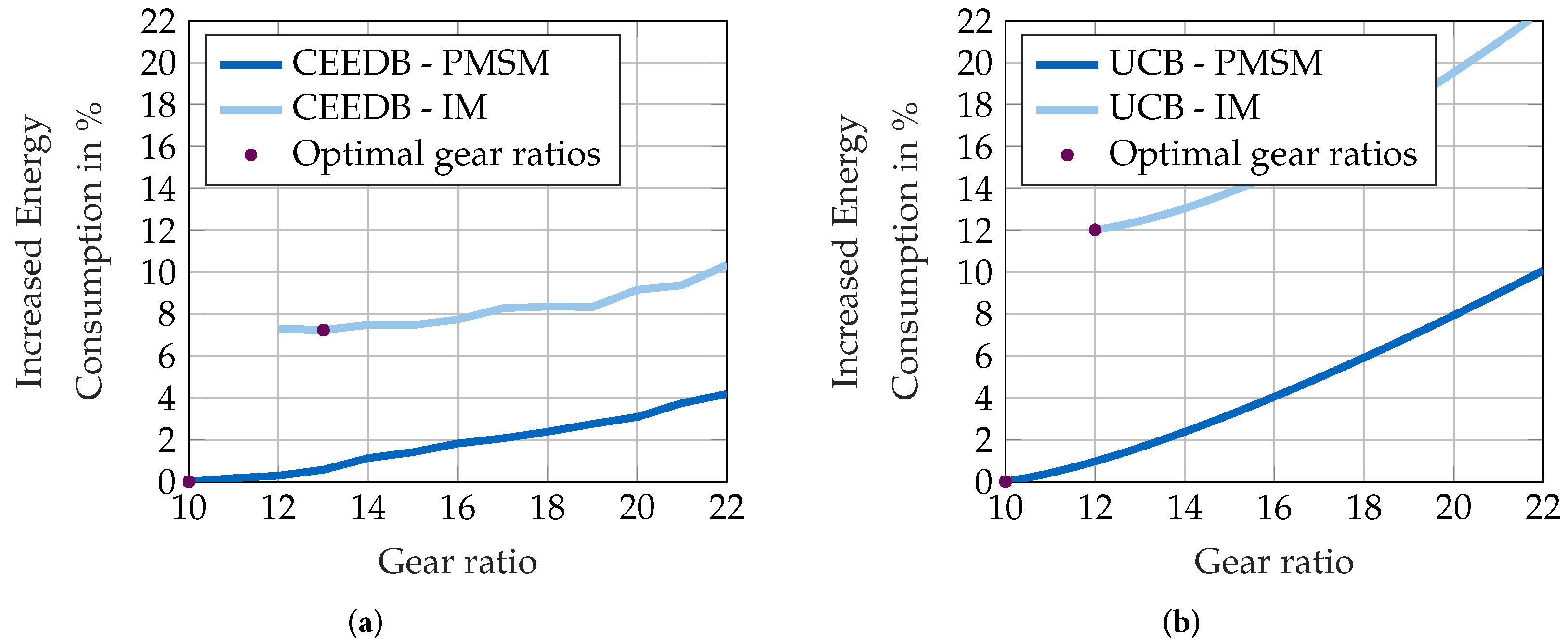
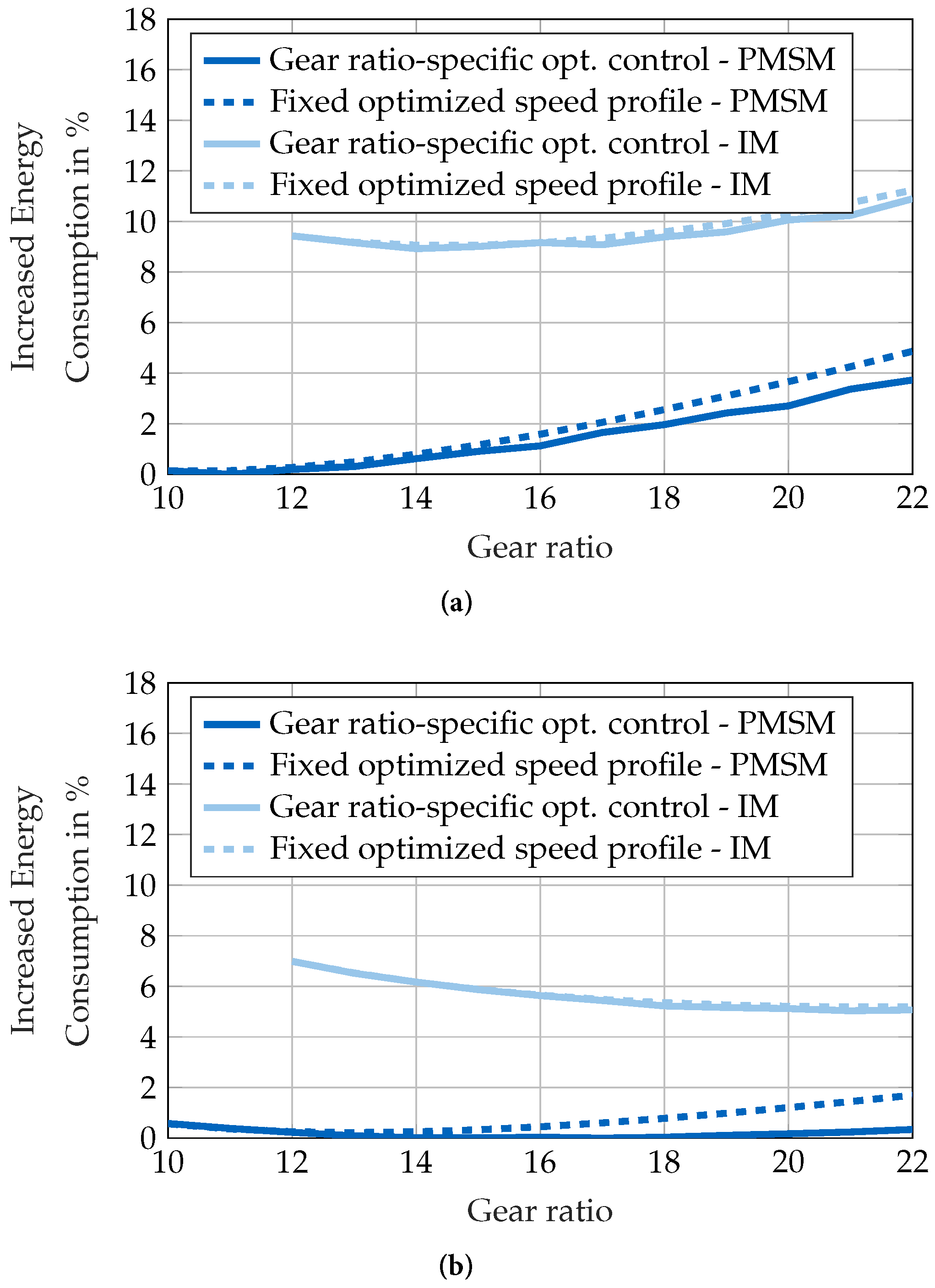
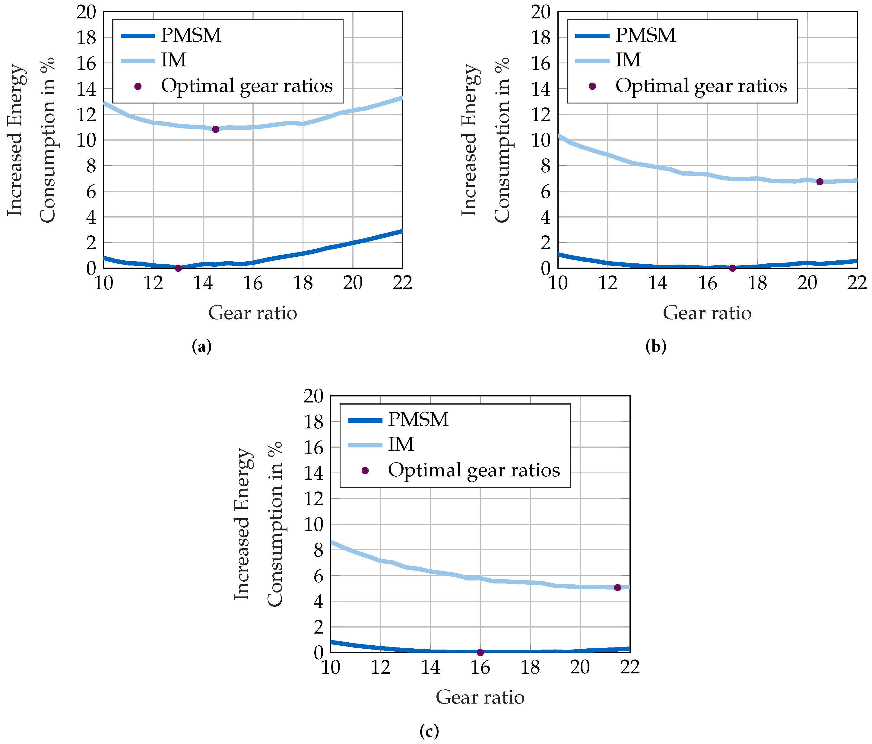
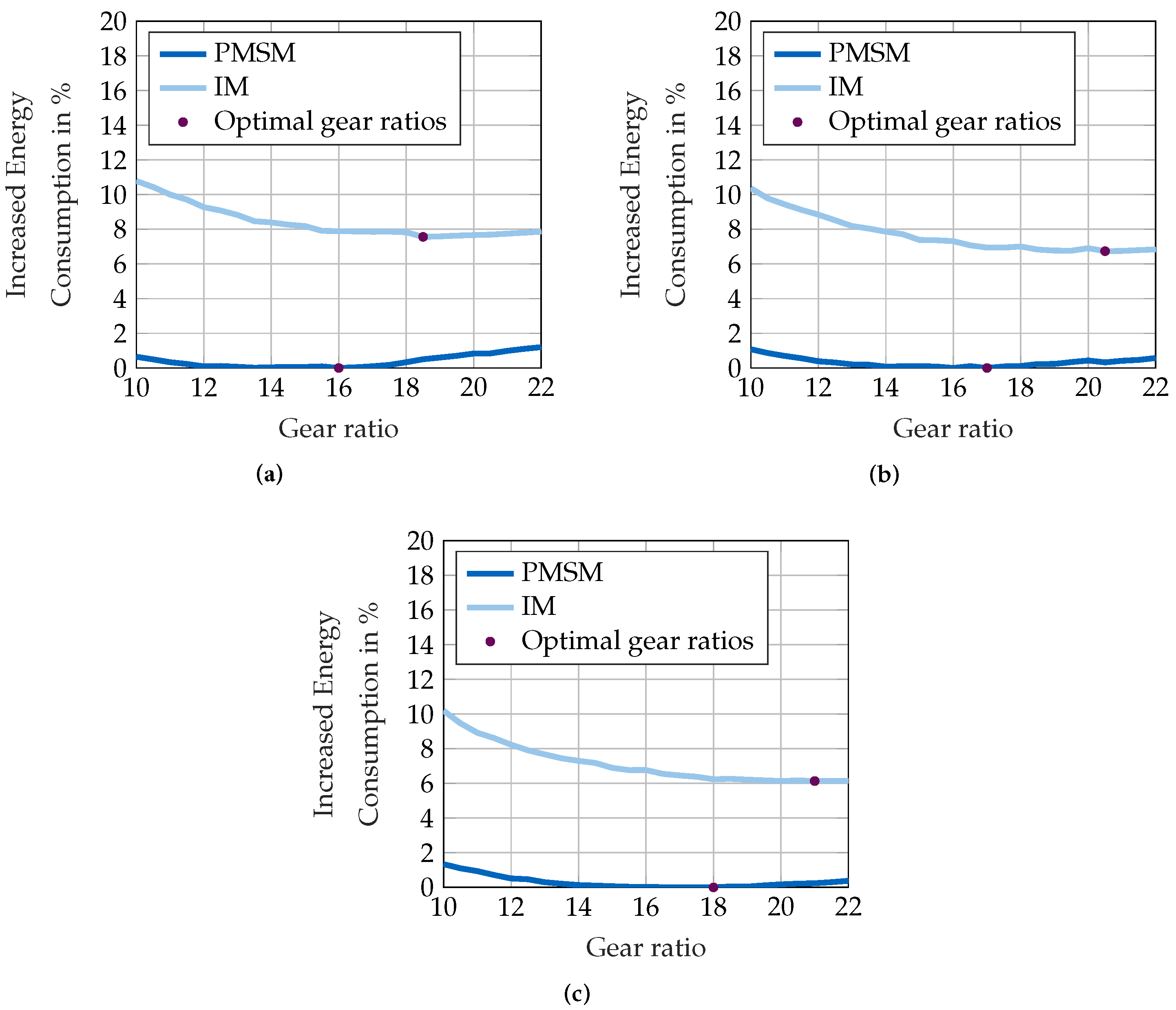
5.3. Effect of Gear Ratios on Energy Consumption
5.4. Limitations
6. Conclusions
Author Contributions
Funding
Conflicts of Interest
Abbreviations
| BEV | Battery electric vehicle |
| CEEDB | Connected energy-efficient driven bus |
| DP | Dynamic programming |
| IM | Induction motor |
| NEDC | New European Driving Cycle |
| P&G | Pulse and glide |
| PMP | Pontryagin’s Maximum Principle |
| PMSM | Permanent magnet synchronous motor |
| UCB | Unconnected bus |
| V2I | Vehicle to infrastructure |
Appendix A

References
- Energy Market Authority. Singapore Energy Statistics 2018. 2018. Available online: https://www.ema.gov.sg/cmsmedia/Publications_and_Statistics/Publications/SES18/Publication_Singapore_Energy_Statistics_2018.pdf (accessed on 11 June 2019).
- NCCS. Land Transport Carbon Emissions by Vehicle Mode (2005). 2019. Available online: https://www.nccs.gov.sg/climate-change-and-singapore/reducing-emissions/transport (accessed on 24 May 2019).
- Authority, L.T. Annual Vehicle Statistics 2018: Motor Vehicle Population By Vehicle Type. 2019. Available online: https://www.lta.gov.sg/content/dam/ltaweb/corp/PublicationsResearch/files/FactsandFigures/MVP01-1_MVP_by_type.pdf (accessed on 24 June 2019).
- Sciarretta, A. Energy-Efficient Driving of Road Vehicles: Toward a Cooperative, Connected, and Automated Mobility; Springer International Publishing: Berlin/Heidelberg, Germany, 2019. [Google Scholar]
- Han, J.; Vahidi, A.; Sciarretta, A. Fundamentals of energy efficient driving for combustion engine and electric vehicles: An optimal control perspective. Automatica 2019, 103, 558–572. [Google Scholar] [CrossRef]
- Eo, J.S.; Kim, S.J.; Oh, J.; Chung, Y.K.; Chang, Y.J. A Development of Fuel Saving Driving Technique for Parallel HEV; SAE Technical Paper Series; SAE International 400 Commonwealth Drive: Warrendale, PA, USA, 2018. [Google Scholar] [CrossRef]
- So, K.M.; Gruber, P.; Tavernini, D.; Karci, A.E.H.; Sorniotti, A.; Motaln, T. On the Optimal Speed Profile for Electric Vehicles. IEEE Access 2020, 8, 78504–78518. [Google Scholar] [CrossRef]
- Lajunen, A. Energy-optimal velocity profiles for electric city buses. In Proceedings of the 2013 IEEE International Conference on Automation Science and Engineering, Madison, WI, USA, 29–30 July 2013; pp. 886–891. [Google Scholar] [CrossRef]
- Kelouwani, S.; Agbossou, K.; Dubé, Y.; Boulon, L. Energetic optimization of the driving speed based on geographic information system data. In Proceedings of the 2012 IEEE Vehicular Technology Conference (VTC Fall), Quebec City, QC, Canada, 3–6 September 2012; pp. 1–5. [Google Scholar]
- Mensing, F.; Trigui, R.; Bideaux, E. Vehicle trajectory optimization for application in ECO-driving. In Proceedings of the 2011 IEEE Vehicle Power and Propulsion Conference, Chicago, IL, USA, 6–9 September 2011; pp. 1–6. [Google Scholar]
- Luu, H.T.; Nouvelière, L.; Mammar, S. Dynamic programming for fuel consumption optimization on light vehicle. IFAC Proc. Vol. 2010, 43, 372–377. [Google Scholar] [CrossRef]
- Nouveliere, L.; Braci, M.; Menhour, L.; Luu, H.; Mammar, S. Fuel consumption optimization for a city bus. In Proceedings of the UKACC Control Conference, Manchester, UK, 1–4 September 2008; pp. 1–6. [Google Scholar]
- Guler, S.I.; Menendez, M.; Meier, L. Using connected vehicle technology to improve the efficiency of intersections. Transp. Res. Part C Emerg. Technol. 2014, 46, 121–131. [Google Scholar] [CrossRef]
- Katsaros, K.; Kernchen, R.; Dianati, M.; Rieck, D. Performance study of a Green Light Optimized Speed Advisory (GLOSA) application using an integrated cooperative ITS simulation platform. In Proceedings of the 2011 7th International Wireless Communications and Mobile Computing Conference, Istanbul, Turkey, 4–8 July 2011; pp. 918–923. [Google Scholar] [CrossRef]
- Amir, G.; Xiaopeng, L.; Zhitong, H.; Xiaobo, Q. A Joint Trajectory and Signal Optimization Model for Connected Automated Vehicles. In Proceedings of the TRB Annual Meeting, Washington, DC, USA, 10–11 July 2019. [Google Scholar]
- Teichert, O.; Koch, A.; Ongel, A. Comparison of Eco-Driving Strategies for Different Traffic-Management Measures. In Proceedings of the 2020 IEEE Intelligent Transportation Systems Conference (ITSC), Rhodes, Greece, 20–23 September 2020; pp. 1867–1873. [Google Scholar]
- Wang, Q.; Santini, D.L. Magnitude and Value of Electric Vehicle Emissions Reductions for Six Driving Cycles in Four US Cities with Varying Air Quality Problems; Technical Report; Argonne National Lab.: Lemont, IL, USA, 1992.
- Thomas, C. Fuel cell and battery electric vehicles compared. Int. J. Hydrog. Energy 2009, 34, 6005–6020. [Google Scholar] [CrossRef]
- Egbue, O.; Long, S. Barriers to widespread adoption of electric vehicles: An analysis of consumer attitudes and perceptions. Energy Policy 2012, 48, 717–729. [Google Scholar] [CrossRef]
- Angerer, C.; Krapf, S.; Buß, A.; Lienkamp, M. Holistic Modeling and Optimization of Electric Vehicle Powertrains Considering Longitudinal Performance, Vehicle Dynamics, Costs and Energy Consumption. In Proceedings of the ASME 2018 International Design Engineering Technical Conferences and Computers and Information in Engineering Conference, American Society of Mechanical Engineers, Quebec City, QC, Canada, 26–29 August 2018; p. V003T01A024. [Google Scholar]
- Ren, Q.; Crolla, D.; Morris, A. Effect of transmission design on Electric Vehicle (EV) performance. In Proceedings of the 5th IEEE Vehicle Power and Propulsion Conference (VPPC’09), Dearborn, MI, USA, 7–11 September 2009; pp. 1260–1265. [Google Scholar] [CrossRef]
- Hofman, I.; Sergeant, P.; Van den Bossche, A. Drivetrain design for an ultra light electric vehicle with high efficiency. In Proceedings of the 2013 World Electric Vehicle Symposium and Exhibition (EVS27), Barcelona, Spain, 17–20 November 2013; pp. 1–6. [Google Scholar] [CrossRef]
- Bottiglione, F.; de Pinto, S.; Mantriota, G.; Sorniotti, A. Energy Consumption of a Battery Electric Vehicle with Infinitely Variable Transmission. Energies 2014, 7, 8317–8337. [Google Scholar] [CrossRef]
- Zeraoulia, M.; Benbouzid, M.E.H.; Diallo, D. Electric Motor Drive Selection Issues for HEV Propulsion Systems: A Comparative Study. IEEE Trans. Veh. Technol. 2006, 55, 1756–1764. [Google Scholar] [CrossRef]
- De Santiago, J.; Bernhoff, H.; Ekergård, B.; Eriksson, S.; Ferhatovic, S.; Waters, R.; Leijon, M. Electrical Motor Drivelines in Commercial All-Electric Vehicles: A Review. IEEE Trans. Veh. Technol. 2012, 61, 475–484. [Google Scholar] [CrossRef]
- Xue, X.D.; Cheng, K.W.E.; Cheung, N.C. Selection of Electric Motor Drives for Electric Vehicles. In Proceedings of the 2008 Australasian Universities Power Engineering Conference, Sydney, Australia, 14–17 December 2008. [Google Scholar]
- Lukic, S.M.; Emado, A. Modeling of electric machines for automotive applications using efficiency maps. In Proceedings of the Electrical Insulation Conference and Electrical Manufacturing and Coil Winding Technology Conference (Cat. No.03CH37480), Indianapolis, Indiana, 23–25 September 2003; pp. 543–550. [Google Scholar] [CrossRef]
- Yang, Z.; Shang, F.; Brown, I.P.; Krishnamurthy, M. Comparative Study of Interior Permanent Magnet, Induction, and Switched Reluctance Motor Drives for EV and HEV Applications. IEEE Trans. Transp. Electrif. 2015, 1, 245–254. [Google Scholar] [CrossRef]
- Goss, J.; Popescu, M.; Staton, D. A comparison of an interior permanent magnet and copper rotor induction motor in a hybrid electric vehicle application. In Proceedings of the 2013 International Electric Machines & Drives Conference, Chicago, IL, USA, 12–15 May 2013; pp. 220–225. [Google Scholar] [CrossRef]
- Pellegrino, G.; Vagati, A.; Boazzo, B.; Guglielmi, P. Comparison of Induction and PM Synchronous Motor Drives for EV Application Including Design Examples. IEEE Trans. Ind. Appl. 2012, 48, 2322–2332. [Google Scholar] [CrossRef]
- Wang, B.; Hung, D.L.S.; Zhong, J.; Teh, K.Y. Energy Consumption Analysis of Different Bev Powertrain Topologies by Design Optimization. Int. J. Automot. Technol. 2018, 19, 907–914. [Google Scholar] [CrossRef]
- Tate, L.; Hochgreb, S.; Hall, J.; Bassett, M. Energy Efficiency of Autonomous Car Powertrain; SAE Technical Paper Series; SAE International 400 Commonwealth Drive: Warrendale, PA, USA, 2018. [Google Scholar] [CrossRef]
- Anselma, P.G.; Belingardi, G. Enhancing Energy Saving Opportunities through Rightsizing of a Battery Electric Vehicle Powertrain for Optimal Cooperative Driving. SAE Int. J. Connect. Autom. Veh. 2020, 3. [Google Scholar] [CrossRef]
- Gambhira, U.R. Powertrain Optimization of an Autonomous Electric Vehicle. Master’s Thesis, The Ohio State University, Columbus, OH, USA, 2018. [Google Scholar]
- Bertsekas, D.P. Dynamic Programming and Optimal Control, 4th ed.; Athena Scientific: Belmont, MA, USA, 2017. [Google Scholar]
- Guzzella, L.; Sciarretta, A. Vehicle Propulsion Systems: Introduction to Modeling and Optimization, 3rd ed.; Springer: Berlin/Heidelberg, Germany, 2013. [Google Scholar] [CrossRef]
- Naunheimer, H.; Bertsche, B.; Lechner, G. Fahrzeuggetriebe. In Grundlagen, Auswahl, Auslegung und Konstruktion./Harald Naunheimer, Bernd Bertsche, Gisbert Lechnerv; Springer: Berlin/Heidelberg, Germany, 2007. [Google Scholar]
- Sundstrom, O.; Guzzella, L. A generic dynamic programming Matlab function. In Proceedings of the 2009 IEEE Control Applications, (CCA) Intelligent Control, (ISIC), Capri, Italy, 9–11 June 2009; pp. 1625–1630. [Google Scholar] [CrossRef]
- Marler, R.T.; Arora, J.S. The weighted sum method for multi-objective optimization: New insights. Struct. Multidiscip. Optim. 2010, 41, 853–862. [Google Scholar] [CrossRef]
- Bae, S.; Kim, Y.; Guanetti, J.; Borrelli, F.; Moura, S. Design and implementation of ecological adaptive cruise control for autonomous driving with communication to traffic lights. In Proceedings of the 2019 American Control Conference (ACC), Philadelphia, PA, USA, 10–12 July 2019; pp. 4628–4634. [Google Scholar]
- Kamal, M.A.S.; Mukai, M.; Murata, J.; Kawabe, T. Ecological driving based on preceding vehicle prediction using MPC. IFAC Proc. Vol. 2011, 44, 3843–3848. [Google Scholar] [CrossRef]
- Wittmann, M.; Lohrer, J.; Betz, J.; Jäger, B.; Kugler, M.; Klöppel, M.; Waclaw, A.; Hann, M.; Lienkamp, M. A holistic framework for acquisition, processing and evaluation of vehicle fleet test data. In Proceedings of the 2017 IEEE 20th International Conference on Intelligent Transportation Systems (ITSC), Yokohama, Japan, 16–19 October 2017; pp. 1–7. [Google Scholar]
- LTA Singapore. Data Mall. Available online: https://www.mytransport.sg/content/mytransport/home/dataMall.html (accessed on 8 May 2019).
- BYD. 12M BATTERY-ELECTRIC BUS—Specifications. Technical Data Sheet. 2019. Available online: http://bydeurope.com/vehicles/ebus/types/12.php (accessed on 27 May 2019).
- Kivekas, K.; Lajunen, A.; Baldi, F.; Vepsalainen, J.; Tammi, K. Reducing the Energy Consumption of Electric Buses With Design Choices and Predictive Driving. IEEE Trans. Veh. Technol. 2019, 68, 11409–11419. [Google Scholar] [CrossRef]
- Kalt, S.; Erhard, J.; Danquah, B.; Lienkamp, M. Electric Machine Design Tool for Permanent Magnet Synchronous Machines. In Proceedings of the 2019 Fourteenth International Conference on Ecological Vehicles and Renewable Energies (EVER), Monte-Carlo, Monaco, 8–10 May 2019. [Google Scholar]
- BYD. 12M BATTERY-ELECTRIC BUS-UNIQUE INNOVATIVE DESIGN. Technical Data Sheet. 2019. Available online: http://bydeurope.com/innovations/technology/index.php#motor (accessed on 8 May 2019).
- LTA Singapore. Civil Design Criteria For Road And Rail Transit Systems. E/GD/09/106/A2. 2019. Available online: https://www.lta.gov.sg/content/dam/ltagov/industry_innovations/industry_matters/development_construction_resources/civil_standards/pdf/EGD09106A2_Overall.pdf (accessed on 5 December 2020).
- Mertens, F. Into the Future with the People Mover. 2018. Available online: https://www.zf.com/mobile/en/stories_7809.html (accessed on 24 November 2020).
- Local Motors. Meet-Olli. 2020. Available online: https://localmotors.com/meet-olli/ (accessed on 24 November 2020).
- Lin, X.; Görges, D.; Liu, S. Eco-driving assistance system for electric vehicles based on speed profile optimization. In Proceedings of the 2014 IEEE Conference on Control Applications (CCA), Nice, France, 8–10 October 2014; pp. 629–634. [Google Scholar]


| Parameter | Bus Route 91 | Bus Route 185 |
|---|---|---|
| Measured route length | 6.0 km | 15.9 km |
| Measured number of bus stops | 13 | 28 |
| Average distance between stops | 460 m | 570 m |
| Number of turns | 14 | 14 |
| Number of traffic lights | 18 | 45 |
| Speed limits | 50 km/h | 50 or 60 km/h |
| Duration | 1612 s | 3766 s |
| Dwelling time | 114 s | 565 s |
| Average speed (without dwelling) | 14.4 km/h | 17.9 km/h |
| Parameter | Value | Source |
|---|---|---|
| Mass | 15,850 kg | [44] |
| Front area | 8.6 m2 | [44] |
| Drag coefficient | 0.7 | assumption |
| Rolling resistance coeff. | 0.008 | [45] |
| Tire radius | 0.48 m | [44] |
| Transmission efficiency | 0.96 | assumption |
| Parameter | Value |
|---|---|
| Nominal voltage | 540 V |
| Max. rotational speed | 7500 U/min |
| Nominal rotational speed | 3500 U/min |
| Type of cooling | liquid |
| Number of pole pairs | 4 |
| Nominal power | 90 kW |
Publisher’s Note: MDPI stays neutral with regard to jurisdictional claims in published maps and institutional affiliations. |
© 2020 by the authors. Licensee MDPI, Basel, Switzerland. This article is an open access article distributed under the terms and conditions of the Creative Commons Attribution (CC BY) license (http://creativecommons.org/licenses/by/4.0/).
Share and Cite
Koch, A.; Teichert, O.; Kalt, S.; Ongel, A.; Lienkamp, M. Powertrain Optimization for Electric Buses under Optimal Energy-Efficient Driving. Energies 2020, 13, 6451. https://doi.org/10.3390/en13236451
Koch A, Teichert O, Kalt S, Ongel A, Lienkamp M. Powertrain Optimization for Electric Buses under Optimal Energy-Efficient Driving. Energies. 2020; 13(23):6451. https://doi.org/10.3390/en13236451
Chicago/Turabian StyleKoch, Alexander, Olaf Teichert, Svenja Kalt, Aybike Ongel, and Markus Lienkamp. 2020. "Powertrain Optimization for Electric Buses under Optimal Energy-Efficient Driving" Energies 13, no. 23: 6451. https://doi.org/10.3390/en13236451
APA StyleKoch, A., Teichert, O., Kalt, S., Ongel, A., & Lienkamp, M. (2020). Powertrain Optimization for Electric Buses under Optimal Energy-Efficient Driving. Energies, 13(23), 6451. https://doi.org/10.3390/en13236451