Combined Economic Emission Dispatch with Environment-Based Demand Response Using WU-ABC Algorithm

Abstract

Owing to the growing interest in environmental problems worldwide, it is essential to schedule power generation considering the effects of pollutants. To address this, we propose an optimal approach that solves the combined economic emission dispatch (CEED) with maximum emission constraints by considering demand response (DR) program. The CEED consists of the sum of operation costs for each generator and the pollutant emissions. An environment-based demand response (EBDR) program is used to implement pollutant emission reduction and facilitate economic improvement. Through the weighting update artificial bee colony (WU-ABC) algorithm, the penalty factor that determines the weighting of the two objective functions is adjusted, and an optimal operation solution for a microgrid (MG) is then determined to resolve the CEED problem. The effectiveness and applicability of the proposed approach are demonstrated via comparative analyses at a modified grid-connected MG test system. The results confirm that the proposed approach not only satisfies emission constraints but also ensures an economically superior performance compared to other approaches. These results present a useful solution for microgrid operators considered environment issues.

1. Introduction

Economic dispatch (ED) is one of the most important issues pertaining to the operation and control of power systems [1,2]. It involves finding an optimal scheduling for all committed generators to minimize fuel costs, while satisfying various constraints such as load demand balance and generation capacity constraints. However, owing to increasing global concerns regarding the environmental issues caused by the combustion of fossil fuels, ED has become a significant concern from an economical perspective and for dealing with pollutant emissions from fossil fuel combustion [3]. Some countries have set maximum emission limits and impose fines when these limits are exceeded [4]. Thus, emission constraints should also be considered during operational scheduling. Economic emission dispatch (EED) has been proposed for scheduling to account for the emission of harmful gases such as carbon dioxide (CO₂), sulfur oxides (SO_x), and nitrogen oxides (NO_x), which pollute the air and exacerbate global warming [5]. The objective function of the EED usually adds emission criteria to the fuel cost of the thermal unit. To integrate the emission component with ED, Dhillon et al. [6] and Kulkarni et al. [7] presented a method whereby a penalty factor is multiplied to the emission term in the objective function. This technique allows both components to become commensurately involved in the optimization.

Demand response (DR) is expected to help solve environmental problems, as it is environmentally friendly and offers several benefits to the entire system [8,9]. This is because DR resources are one of the most inexpensive resources and can react quickly to the commands of the system operator [10]. Furthermore, they do not emit pollutants and help reduce peak loads. In a DR program, consumers sign a contract with the local utility to reduce their demand when requested by the system operator. The utility possesses the advantage of reducing the maximum demand and consequently decreasing operation costs. Moreover, the system operator can use the DR program to satisfy constraints such as maximum pollutant emissions. DR programs are commonly used in small power systems such as microgrids (MGs), because they are difficult to implement in large power systems due to communication problems [11,12].

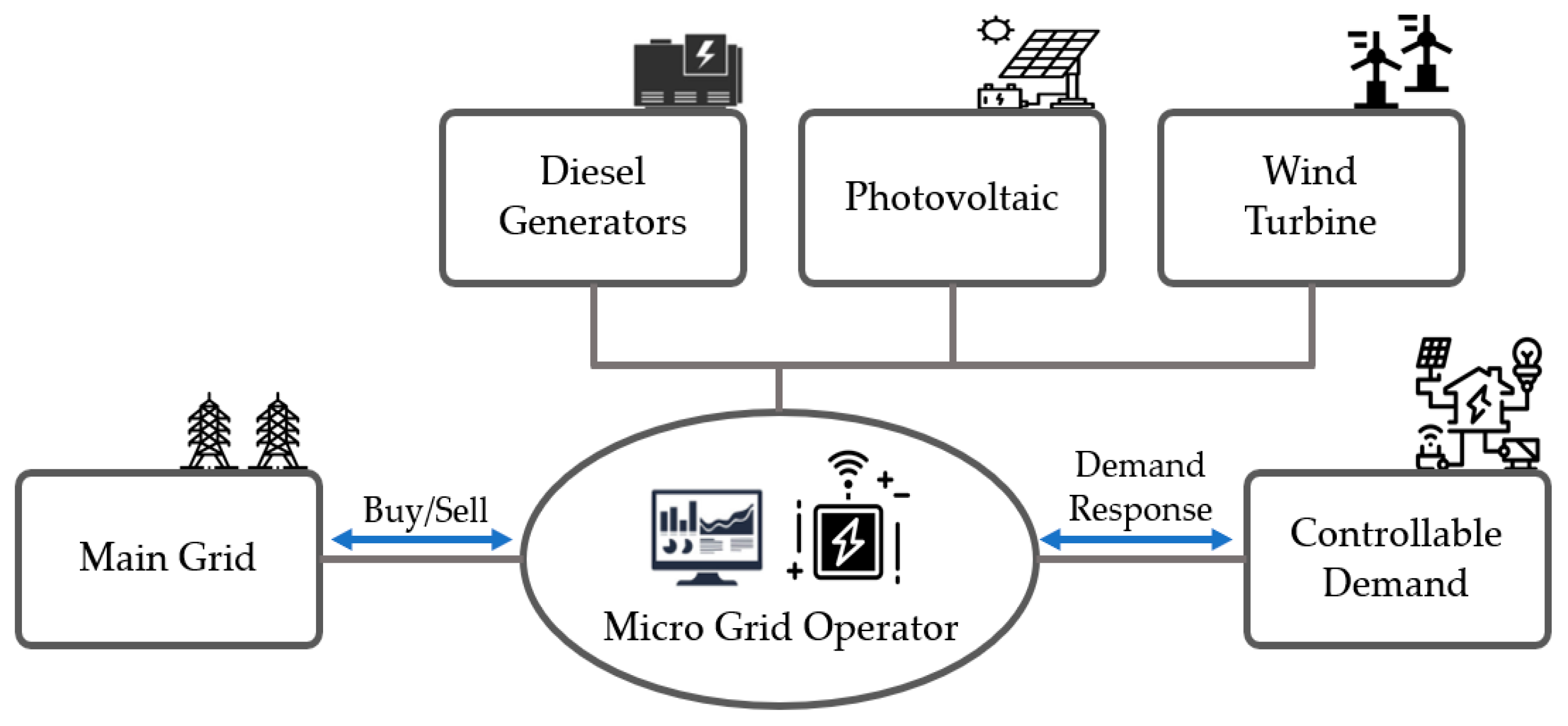
MGs can be defined as a small-scale form of the centralized power system and typically consist of diesel generation (DG) units, renewable energy resources, and loads that are designed and situated close to customers in small communities [13]. MG operators (MGOs) manage a cluster of loads and power resources, conducting operations to control power locally. MGOs also create contracts with the utility service to meet environmental constraints of the EED, and they take the maximum emission constraints into account in the context of MG operation. To satisfy such constraints, ecofriendly energy resources such as DR should be used appropriately.

Various approaches have been recently adopted to address environmental problems in MG operation. In [14], emissions of harmful gases such as CO₂, SO_x, and NO_x were reduced by installing additional ecofriendly generators that consume less fuel. In [15], a differential evolution technique that combines heat and power was proposed to solve the microgrid economic and emission dispatch problem. In [16], both emission and fuel costs were implemented through different variants of particle swarm optimization. A hybrid algorithm that combines the differential evolution algorithm and particle cluster optimization was used to solve the EED problem [17]. In [18], a price penalty factor, which is the ratio between the maximum fuel cost and the maximum emission of the corresponding generator, was applied for solving the EED problem. However, the studies mentioned above did not take the DR program into account, and the optimal operations were insufficient under environmental considerations. In [19], a multi-objective approach was proposed to optimize microgrid in a short-term with renewable energy sources with a randomized natural behavior. However, pollutant emissions was not considered. Through the implementation of the DR program, in [20], a balanced solution was obtained where a sample hub energy system containing conventional and renewable energy sources was solved with a mixed integer linear program for optimizing operation costs and reducing pollutant emission. In [21], extended game theory was incorporated into the multiobjective dynamic EED optimization problem through a DR model. In [22,23], DR was considered for spinning reserves to solve the EED problem. However, the cost of interruptions and the incentives of the participating subjects were not considered.

Several methods have been considered to solve the EED problem. A flower pollination algorithm was used to solve economic load dispatch and EED problems by considering the power limits of the generator [24]. In [25], economic load and emission dispatch were determined with a bioinspired algorithm in a renewable integrated islanded MG. A converted single objective function comprising fuel cost and emission was optimized using a gravitational search algorithm in [26]. In [27], quantification of the impacts of the CO2 emission has been considered on the planning, economic and scheduling decisions. While most EED problems include pollutant emissions in the objective function, there were no maximum emission constraints on the power system. To operate MGs while accounting for environmental concerns, because maximum emission constraints are practically essential, the optimal operation approach for these problems must be studied. In addition, DR is a considerably ecofriendly energy resource; however, very few studies focus on it to determine volume with respect to environmental constraints. Therefore, it is essential to conduct a study on the optimization of MG operation by utilizing a DR program and considering emission constraints for combined economic emission dispatch (CEED) problems.

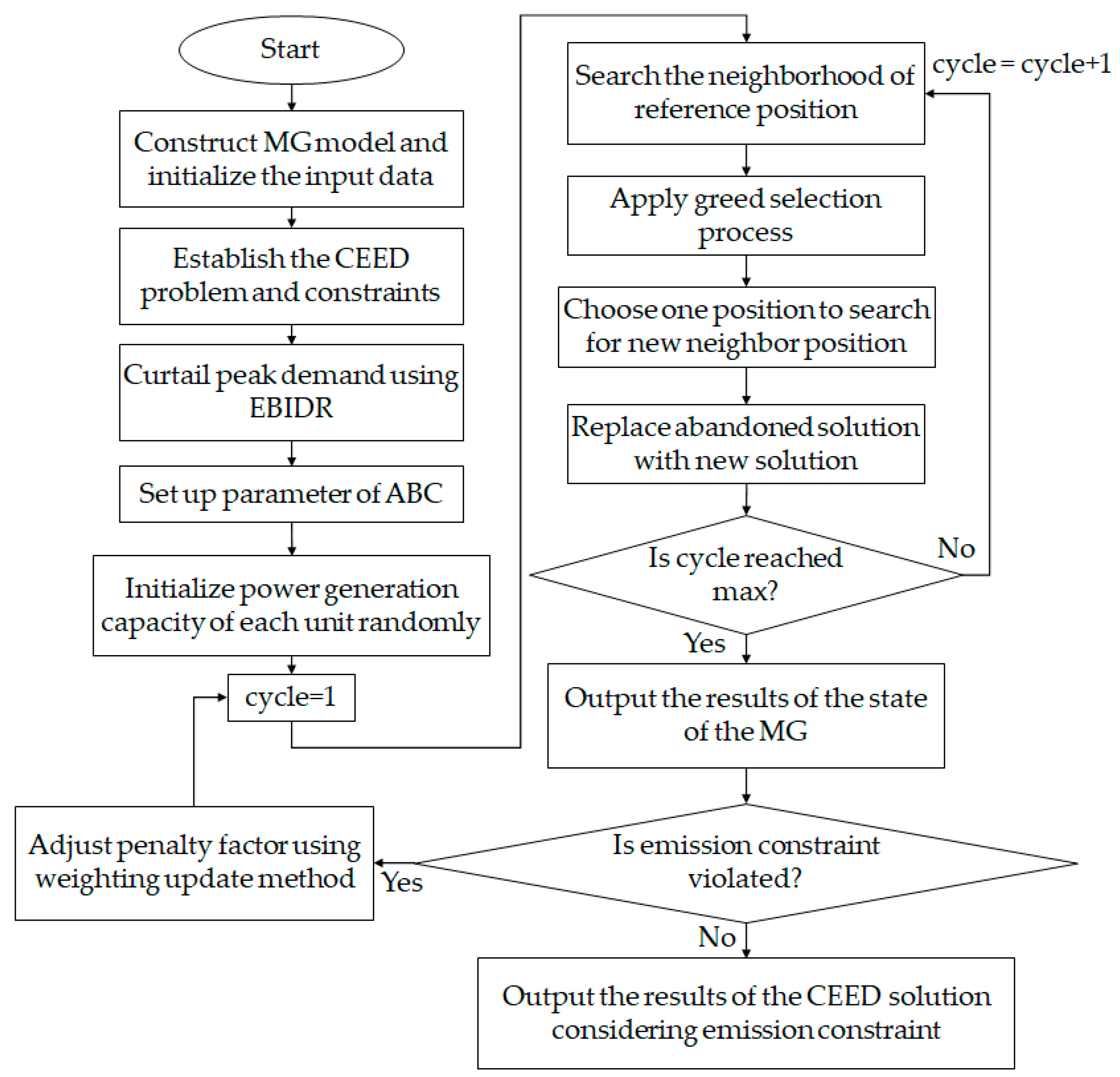
In this study, we propose an approach to solve the CEED problem while considering maximum emission constraints. The CEED function consists of the operation costs and pollutant emissions. Here, the penalty factor is used to convert the emission into an equivalent cost value. Various constraints are considered in solving the problem. In particular, the maximum emission constraint is additionally considered. To solve this problem optimally, we propose an environment-based demand response (EBDR) program that determines volume by optimizing economics and reducing the degree of pollutant emissions from the system. A weighting update artificial bee colony algorithm (WU-ABC) is applied to solve the CEED problem under a maximum emission constraint. Here, the penalty factor is updated using the weighting update method until all the constraints are satisfied. By using WU-ABC algorithm, the proposed approach becomes capable of finding the optimal CEED solution of the MG.

The primary contributions of this paper can be summarized as follows:

• The CEED problem, with a maximum emission constraint on the MG, involves the minimization of operation costs and pollutant emissions. A penalty factor is used by the MGO to control the importance of both objective functions with respect to pollutant emissions. This approach is sufficiently effective to satisfy the maximum emission constraints on MG operation.
• EBDR is applied and both economic and environmental factors are considered. Through the concept of elasticity, the MGO can command demand shifts and reduction, and participants in the DR program are provided appropriate incentives. Through this EBDR program, economics can be improved and environmental hazards can be reduced.
• To solve the CEED problem, we propose the use of the WU-ABC algorithm. This algorithm can efficiently update the penalty factor according to the maximum emission constraint by using the weighting update method in combination with the ABC algorithm, which has been widely used for the optimal operation of power systems of late.

The proposed approach provides an optimal power scheduling using EBDR for MG systems in CEED problems with maximum emission constraints. In this regard, MGOs can be provided with more reasonable and flexible solutions for optimal operation with environmental constraints.

The remainder of this paper is organized as follows. Section 2 introduces the grid-connected MG system model. Section 3 presents the formulation of the problem for the CEED with a maximum emission constraint. Section 4 outlines the proposed EBDR strategy. Section 5 presents the solution of the WU-ABC algorithm and summarizes the overall process. Section 6 presents the simulation results, and Section 7 presents the conclusions of this study.

2. Grid-Connected MG System

Figure 1 shows the structure of the proposed grid-connected MG that includes DG, photovoltaic (PV), wind turbine (WT) units and controllable demands; it is connected to the main grid. MGOs can sell surplus power or buy insufficient power through interactions with the main grid, and they can request demand reduction from the customers using the DR program [28,29].

2.1. DG Model

The power generation costs of a diesel generator are generally expressed as the sum of a quadratic and sinusoidal function.

$$C_{G,i}(t)=a_i{P}_{G,i}^2(t)+b_i{P}_{G,i}(t)+c_i+\left|d_i\sin [P_{G,i}^{\min }(t)-P_{G,i}(t)]\right|$$

(1)

Here, the sinusoidal function represents a valve point effect to practically account for the generation cost function. Figure 2 illustrates the valve point effect for a conventional generator. It represents a sharp increase in losses due to the wire drawing effect caused by the opening of each steam admission valve [30].

2.2. PV Model

The output power of a PV is dependent on solar irradiation. Forecasted solar irradiation is commonly determined using the beta probability distribution function (PDF) expressed as follows [31].

$$PD{F}_B(si)=\{\begin{array}{c}\frac{\mathsf{\Gamma }(a+b)}{\mathsf{\Gamma }(a)\mathsf{\Gamma }(b)}\hspace{0.17em}·\hspace{0.17em}s{i}^{(a-1)}·\hspace{0.17em}{(1-si)}^{(b-1)}\\ 0\end{array}\hspace{0.17em}\hspace{0.17em}\hspace{0.17em}\hspace{0.17em}\begin{array}{c}0\le si\le 1\hspace{0.17em},\hspace{0.17em}a\ge 0\hspace{0.17em},\hspace{0.17em}b\ge 0\\ otherwise\end{array}$$

(2)

$$a=\frac{{\mu }_s\times b}{1-{\mu }_s}\hspace{0.17em}\hspace{0.17em}\hspace{0.17em}$$

(3)

$$b\hspace{0.17em}=\hspace{0.17em}(1-{\mu }_s)\times \left(\frac{{\mu }_s\times (1+{\mu }_s)}{{\sigma }_s{}^2}-1\right)$$

(4)

The shape parameters a and b are determined according to the mean (μ_s) and standard deviation (σ_s) of solar irradiation data.

Mathematically, the generated power from the PV array is represented as

$$P_s(t)={\eta }_s\times A_s\times SI(1+\beta (T_t-25))$$

(5)

The generated solar power is represented by the product of PV panel efficiency, size of the PV array, and solar irradiation. β denotes temperature coefficients of the maximum power of the PV array.

2.3. WT Model

The Weibull PDF has been regularly used to model wind speed and can be expressed as

$$PD{F}_w(v)=\left(\frac{d}{C}\right){\left(\frac{v}{C}\right)}^{d-1}\hspace{0.17em}\exp \hspace{0.17em}\left[-{\left(\frac{v}{C}\right)}^d\right]$$

(6)

The hourly output of a WT unit is highly dependent on wind speed. The mathematical expression for converting the hourly wind speed to power is as follows:

$$P_w(t)=\{\begin{array}{cc}0& if\hspace{0.17em}\hspace{0.17em}\hspace{0.17em}{v}_t<v_{ci}\hfill \\ P_r\times \frac{(v_t-v_{ci})}{(v_r-v_{ci})}& if\hspace{0.17em}\hspace{0.17em}\hspace{0.17em}{v}_{ci}\le v_t<v_r\hfill \\ P_r& if\hspace{0.17em}\hspace{0.17em}\hspace{0.17em}{v}_r\le v_t<v_{co}\hfill \\ 0& if\hspace{0.17em}\hspace{0.17em}\hspace{0.17em}{v}_{co}\le v_t\hfill \end{array}$$

(7)

2.4. Utility Model

For MG operation, MGOs purchase deficit energy from the main grid depending on price and internal generation levels. Conversely, they sell excess energy to the main grid. The amount of power and exchange cost traded between the utility and the MG in each hour is expressed as:

$$P_u(t)=P_{buy}(t)\hspace{0.17em}{b}_u(t)-P_{sell}\hspace{0.17em}(b_u(t)-1))$$

(8)

$$C_u(t)=\{\begin{array}{c}{\lambda }_{sell}(t)\times P_u(t)\\ 0\\ {\lambda }_{buy}(t)\times P_u(t)\end{array}\hspace{0.17em}\hspace{0.17em}\hspace{0.17em}\hspace{0.17em}\hspace{0.17em}\hspace{0.17em}\hspace{0.17em}\begin{array}{c}if\hspace{0.17em}\hspace{0.17em}\hspace{0.17em}{P}_u(t)<0\\ if\hspace{0.17em}\hspace{0.17em}\hspace{0.17em}{P}_u(t)=0\\ if\hspace{0.17em}\hspace{0.17em}\hspace{0.17em}{P}_u(t)>0\end{array}$$

(9)

Here, the power generation state of the MG b_u(t) takes the value 1 when there is a deficit in power, and 0 when there is a surplus of power.

3. Problem Formulation

In the optimization for the CEED problem, two competing objective functions are mathematically formulated by nonlinear functions, which minimize both generation costs and emission function by fulfilling the equality and inequality constraints. In other words, the problem is formulated for the multiobjective function as the minimization of the operation costs and pollutant emissions. The emission function is converted to cost by a multiplying with a weight called the penalty factor.

3.1. Objective Function

3.1.1. Generation Cost Function

The generation cost function is the sum of costs for each generator, including renewable energy source (RES). Conventional generators such as thermal generating units are generally expressed as the sum of a quadratic and sinusoidal function. Costs for PV and WT units, such as the available RES, are determined by considering investment and maintenance costs. The operation costs can be formulated as:

$$F(P)={\displaystyle \sum _{t=1}^{24}[{\displaystyle \sum _{i=1}^I{C}_{G,i}(t)}}+{\displaystyle \sum _{j=1}^J{C}_{s,j}{P}_{s,j}}(t)+{\displaystyle \sum _{k=1}^K{C}_{w,k}{P}_{w,k}(t)+C_u(t)}]$$

(10)

$$P={[P_{G,1},\dots ,P_{G,I},P_{s,1},\dots ,P_{s,J},P_{w,1},\dots ,P_{w,K}]}^T$$

(11)

$$C_{s,j}=A{C}_{s,j}{I}_{s,j}+G_{s,j}$$

(12)

$$C_{w,k}=A{C}_{w,k}{I}_{w,k}+G_{w,k}$$

(13)

Equation (11) denotes the vector of the real power output of each generator. Equations (12) and (13) represent the costs of power generation with renewable energy sources, which include installation and maintenance costs. AC is an annuitization coefficient, and it can be calculated using the following equation [32]:

$$AC=\frac{r}{1-{(1+r)}^{-N}}$$

(14)

3.1.2. Emission Function

The quantity of atmospheric pollutants, such as CO₂, SO_x, and NO_x emitted by a conventional generator can be expressed as the sum of a quadratic and exponential function:

$$E(P)={\displaystyle \sum _{t=1}^{24}em(t)=}{\displaystyle \sum _{t=1}^{24}{\displaystyle \sum _{i=1}^I[\{{\alpha }_i{P}_{G,i}^2(t)+{\beta }_i{P}_{G,i}(t)+{\gamma }_i+{\zeta }_i\exp ({\lambda }_i{P}_{G,i}(t))\}}}]$$

(15)

In Equation (15), the emission dispatch function is considered as a convex polynomial, similar to the operation cost function. In addition, it is assumed that RES is not considered in the emission function because it does not release air pollutants [33].

3.1.3. Combined Economic Emission Dispatch

As discussed above, the generation costs and emission dispatch function are two different objectives. Hence, a compromise solution is required to solve the CEED problem that minimizes generation costs and the emitted quantities of pollutants. To solve a multiobjective function, a penalty factor is used to reform the emission criteria into the generation cost. Mathematically, the penalty factor is a multiplied value that transforms two different functions into a single objective function. In our work, a DR program is considered for microgrid operation. Therefore, the costs of participating in the DR program are included in the CEED problem, as follows.

$$C(P)=\min \hspace{0.17em}{\displaystyle \sum _{t=1}^{24}{\displaystyle \sum _{i=1}^I[F(P)+h_i\times E(P)+C_{DR}(t)]}}$$

(16)

$$C_{DR}(t)=I(\Delta D(t))+P(\Delta D(t))$$

(17)

Here, the penalty factor h_i indicates the ratio ($/kg) of the generation costs and emission quantity of each generator i. This factor is initially determined by considering the minimum and maximum of each objective function, and then it is updated to account for environmental constraints. Equation (13) indicates the costs of participating in the DR program; it includes incentive and penalty costs. In this paper, it is determined based on the proposed EBDR program.

3.2. Constraints

3.2.1. Generation Capacity Constraint

The power output of each generation unit is restricted by lower and upper limits for stable operation:

$$P_{G,i}^{\min }(t)\le P_{G,i}(t)\le P_{G,i}^{\max }(t)$$

(18)

$$P_u^{\min }(t)\le P_u(t)\le P_u^{\max }(t)$$

(19)

$$P_{s,j}^{\min }(t)\le P_{s,j}\le P_{s,j}^{\max }(t)$$

(20)

$$P_{w,k}^{\min }(t)\le P_{w,k}(t)\le P_{w,k}^{\max }(t)$$

(21)

Equations (18)–(21) indicate the minimum and maximum power limits of DG, utility, PV, and WT, respectively.

3.2.2. Power Balance Constraint

The total power generation must cover the total power demand in the presence of transmission line loss:

$${\displaystyle \sum _{i=1}^I{P}_{G,i}}(t)+{\displaystyle \sum _{j=1}^J{P}_{PV,j}(t)}+{\displaystyle \sum _{k=1}^K{P}_{WT,k}(t)}=P_D(t)-P_{loss}(t)$$

(22)

$$P_D(t)=D_0(t)+\Delta D(t)$$

(23)

Equation (23) represents the power demand that is finally determined through the DR.

3.2.3. DR Capacity Constraints

The DR capacity is determined by the contract between the MGO and the customers, and it cannot exceed the maximum capacity:

$$\Delta D(t)\le \Delta D^{\max }(t)$$

(24)

3.2.4. Transmission Line Constraints

For stable operation, MGO should consider the transmission line constraint. The upper limit of the transmission line is as follows:

$$S_l\le S_l^{\max },\hspace{0.17em}\hspace{0.17em}\hspace{0.17em}\hspace{0.17em}\hspace{0.17em}\hspace{0.17em}l=1,\dots ,L$$

(25)

3.2.5. Emission Constraints

The proposed CEED problem takes into account maximum emission constraints to prevent air pollution. If the MGOs violate emission constraints, they will have to pay a fee for the volume of excess.

$$em(t)\le e{m}^{\max }(t)$$

(26)

4. Environment-Based Demand Response Program

This paper proposes a new type of incentive DR program called EBDR with emission control measures by including emission constraints. Generally, aiming to reduce peak demand, the MGO uses DR programs to adjust consumer behavior and manage power demand. The DR program includes the modification of electricity consumption patterns and incentives to promote this change. Demand and pollutant emission are directly related during MG operation. Thus, when solving the CEED problem, the EBDR is used to control pollutant emissions as well as reduce peak demand for economic benefits. By utilizing EBDR, MGOs can operate the MGs in an ecofriendly manner.

4.1. Price Elasticity of Demand

The EBDR includes the concept of elasticity based on market price. Elasticity is a measure used in economics to assess the percentage of change in demand caused by price fluctuations. In terms of power consumption, this percentage changes as the power demand varies with the changes in market prices, which is defined as an increase in price over time and not an absolute value. Elasticity is expected to be negative because higher power prices can cause demand reductions. The elasticity of the demand for electricity is calculated as follows:

$$E(t_1,t_2)=\frac{M{P}_0(t_2)}{D_0(t_1)}\times \frac{\partial D(t_1)}{\partial MP(t_2)}\hspace{0.17em},\hspace{0.17em}\hspace{0.17em}\hspace{0.17em}\hspace{0.17em}\hspace{0.17em}\hspace{0.17em}{t}_1,t_2=1,2\dots ,24$$

(27)

Two types of elasticity of demand exist: self-price elasticity and cross-elasticity [34,35]. Self-price elasticity disregards the shift in demand from one period to another and considers changes in consumption over a given period. In this case, increments in market price lead to demand reduction, and self-elasticity always has a negative value. Meanwhile, cross-elasticity is the transferred demand from the peak period to the off-peak demand period within a day. When t₁ is not equal to t₂, the price drop at t₂ causes a demand reduction at t₁. Thus, cross-elasticity always has a positive value.

$$\{\begin{array}{c}E(t_1,t_2)\le 0\\ E(t_1,t_2)>0\end{array}\hspace{0.17em}\hspace{0.17em}\hspace{0.17em}\hspace{0.17em}\hspace{0.17em}\hspace{0.17em}\begin{array}{c}if\hspace{0.17em}\hspace{0.17em}\hspace{0.17em}{t}_1=t_2\\ if\hspace{0.17em}\hspace{0.17em}\hspace{0.17em}{t}_1\ne t_2\end{array}$$

(28)

4.2. Modeling of EBDR

The MGO enters into contracts with the customers through the EBDR program and mentions the values of incentive and penalty. The customers change their demand from D₀(t) to D(t) according to the contract. The values of incentive and penalty for DR are given by

$$\Delta D(t)=D(t)-D_0(t)$$

(29)

$$I(\Delta D(t))=inc(t)·[D_0(t)-D(t)]$$

(30)

$$P(\Delta D(t))=pen(t)·\left\{CP(t)-\left[D_0(t)-D(t)\right]\right\}$$

(31)

Equation (29) represents the shift in demand of a customer due to the contract. Equations (30) and (31) denote the total values of incentive and penalty, respectively.

The EBDR program shifts the peak demand to reduce operation costs using cross-elasticity based on market prices. The relationship between market prices and demand is represented as follows:

$$D(t_1)=D_0(t_1)+{\displaystyle \sum _{t_1=1}^{24}E(t_1,t_2)·\frac{D_0(t_1)}{M{P}_0(t_2)}·[MP(t_2)-M{P}_0(t_2)]\hspace{0.17em}\hspace{0.17em}\hspace{0.17em}\hspace{0.17em}\hspace{0.17em}\hspace{0.17em}if\hspace{0.17em}\hspace{0.17em}\hspace{0.17em}{t}_1\ne t_2}$$

(32)

Equation (32) represents the power demand at t₁ according to the market price at t₂, considering a 24-h interval. When incentive and penalty are included in the price, the formula is modified as follows:

$$D(t_1)=D_0(t_1)\left\{1+{\displaystyle \sum _{\begin{array}{c}{t}_1=1\hspace{0.17em}\hspace{0.17em}\\ t_1\ne t_2\end{array}}^{24}E(t_1,t_2)·\frac{\left[MP(t_2)-M{P}_0(t_2)+inc(t_2)+pen(t_2)\right]}{M{P}_0(t_2)}}\right\}$$

(33)

Equation (33) indicates only the change in demand due to the market price, without considering emission constraints. The change in demand when emission constraints are included is calculated by utilizing the concept of self-elasticity as follows:

$$\{\begin{array}{cc}{D}_e(t_1)=D(t_1)+E_e(t_1,t_1)·\frac{D(t_1)}{e{m}_{\max }(t)}·[em(t_1)-e{m}_{\max }(t)]& if\hspace{0.17em}\hspace{0.17em}\hspace{0.17em}em(t_1)>e{m}_{\max }(t_1)\hfill \\ D_e(t_1)=D(t_1)& if\hspace{0.17em}\hspace{0.17em}\hspace{0.17em}em(t_1)\le e{m}_{\max }(t_1)\hfill \end{array}$$

(34)

Here, emission constraints are imposed when emissions are greater than the set emission limit. The above equation yields the 24-h interval consumption of customers participating in the EBDR program, in order to minimize MG operating costs while considering emission constraints.

5. Solution Method

WU-ABC Optimization

In this study, we propose a solution through the WU-ABC algorithm, a hybrid of the weighting update method and the ABC algorithm, to solve the CEED optimization problem. The ABC algorithm is a swarm-based optimization method that simulates the foraging behavior of a bee swarm; it has recently been used in many studies to solve optimization problems [36,37]. However, it is difficult to solve the proposed CEED problem under emission constraints using the ABC algorithm alone. Therefore, the weighting update method is also employed to solve the emission problem by adjusting the penalty factor and EBDR capacity. The WU-ABC algorithm involves five main steps, as described below:

• Initialization step: In this step, the initial population of food source is placed randomly in a D-dimensional problem space.

  $$x_{mn}=x_{mn}^{\min }+rand[0,1]·(x_{mn}^{\max }-x_{mn}^{\min })$$

  (35)
  Equation (35) represents the m^th random food source of dimension n in the CEED problem.
• Employed bees step: Each bee repeatedly explores a food source to find the optimal solution, and then it chooses a new optimal position (v_mn) close to the reference position.

  $$v_{mn}=x_{mn}^{}+{\varphi }_{mn}·(x_{mn}^{}-x_{on}^{}),\hspace{0.17em}\hspace{0.17em}\hspace{0.17em}\hspace{0.17em}\hspace{0.17em}\hspace{0.17em}\hspace{0.17em}m\ne o$$

  (36)
  When an employed bee finds a food source that is better than the reference one (x_mn), the reference food source is superseded with the new candidate.
• Onlooker bees step: Onlooker bees look for new positions that are close to the old position through a greedy search method. The bees consider a fitness value, the amount of nectar, and probabilistically determine the space for their next exploration, as follows:

  $$P_m=\frac{fi{t}_m}{{\displaystyle \sum _{m=1}^{SN}fi{t}_m}}$$

  (37)
  In Equation (37), fit_m is a value that is proportional to the amount of nectar.
• Scout bee step: If the reference solution cannot be improved through the number of predetermined trials, this food source is abandoned, and the scout bee tries to find a new food source to replace the abandoned food source. The new food source in the solution space is determined using Equation (35). This process is repeated for maximum cycles.
• Weighting update step: This step is executed when an optimal solution violates the emission constraint. The penalty factor is updated as much as the actual pollutant emission exceeds the maximum emission, through a weight adjustment method. This process is repeated until the pollutant emission constraints are satisfied for optimal MG operation. Multiplication by a linear function is generally used as the weight update rule. In our work, to improve the convergence speed and accuracy, we use multiplication with an exponential function for the weighting update, as follows:

  $$h(s+1)=h(s)\times \exp \left[\eta \times \left(\frac{em(s)-e{m}^{\max }(s)}{e{m}^{\max }(s)}\right)\right]\hspace{0.17em}\hspace{0.17em}\hspace{0.17em}\hspace{0.17em}\hspace{0.17em}\hspace{0.17em}\hspace{0.17em}\hspace{0.17em}\hspace{0.17em}\hspace{0.17em}\hspace{0.17em}if\hspace{0.17em}\hspace{0.17em}\hspace{0.17em}em(s)>e{m}^{\max }(s)$$

  (38)

After updating the penalty factor using Equation (38), optimization is performed again through the ABC algorithm.

Figure 3 summarizes the proposed CEED solution. The procedure is performed sequentially as follows:

Step 1:

Construct the MG model comprising DG, PV, and WT units and controllable demand, as shown in Figure 1, and initialize the input data for Equations (1)–(9).

Step 2:

Establish the CEED problem and constraints according to Equations (10)–(26).

Step 3:

Curtail the peak demand using EBDR as a base for elasticity from Equations (27)–(33).

Step 4:

Set up parameters of the ABC algorithm, including the number of populations, maximum cycle, and maximum exploration.

Step 5:

Initialize the power generation capacity of each unit randomly based on the initialization step in Equation (35).

Step 6:

Search the neighborhood of the refence position through the employed bees, using Equation (36).

Step 7:

Subject to Equation (37), apply a greedy search and choose one position to subsequently search for new neighboring positions.

Step 8:

Replace the abandoned solution with the new solution found by the scout bees.

Step 9:

Check that the result does not violate the emission constraint.

Step 10:

If the emission constraint is violated, adjust the penalty factor in Equation (38).

Step 11:

Repeat this process until the MG has satisfied all constraints.

Figure 3. Overall process of the combined economic emission dispatch (CEED) solution.

Figure 3. Overall process of the combined economic emission dispatch (CEED) solution.

6. Simulation Results

6.1. System Data

To verify the effectiveness and validity of the proposed approach, a simulation is conducted on the modified grid-connected MG system consisting of three DG units, one 40-MW PV system, and one 30-MW wind farm [25].

Table 1. Diesel generation (DG) profiles.

DG Source	Min Power (MW)	Max Power (MW)	ai ($/MW2h)	bi ($/MWh)	ci ($/h)	αi (kg/MW2h)	βi (kg/MWh)	γi (kg/h)
G1	30	120	0.024	21	0	0.0105	−1.355	60
G2	32	128	0.029	20.16	0	0.008	−0.6	45
G3	40	152	0.021	20.4	0	0.012	−0.555	90

lists each DG characteristic, including the min/max power limit, generation costs, and emission coefficients [32]. The operation costs for the wind farm and PV system include maintenance and investment costs of 30.8$/MWh and 23.4$/MWh, respectively [32].

Table 2. Demand and forecasted hourly output of RES.

Time (h)	Demand (MW)	PV (MW)	WT (MW)
1	140	0	1.7
2	150	0	8.5
3	155	0	9.27
4	160	0	16.66
5	165	0	7.22
6	170	0.03	4.91
7	175	6.27	14.66
8	180	16.18	25.56
9	210	24.05	20.58
10	230	39.37	17.85
11	240	7.41	12.80
12	250	3.65	18.65
13	240	31.94	14.35
14	220	26.81	10.35
15	200	10.08	8.26
16	180	5.30	13.71
17	170	9.57	3.44
18	185	2.31	1.87
19	200	0	0.75
20	240	0	0.17
21	225	0	0.15
22	190	0	0.31
23	160	0	1.07
24	145	0	0.58

depicts the hourly demand and generation power of RES, which are calculated for wind speeds and solar irradiation in the east coast of the USA [32].

Table 3. Market price and DR incentive.

Time (h)	Market Price (MW)	DR Incentive (MW)	Time (h)	Market Price (MW)	DR Incentive (MW)
1	30.70	27.30	13	69.90	35.50
2	25.70	26.70	14	64.10	38.80
3	21.40	26.50	15	60.00	38.10
4	17.30	28.20	16	52.00	38.10
5	14.90	27.50	17	39.10	37.50
6	16.60	27.60	18	32.20	36.50
7	16.10	29.70	19	29.50	35.70
8	16.60	29.20	20	27.20	34.50
9	26.40	30.10	21	15.20	33.80
10	32.70	31.90	22	12.10	29.80
11	36.50	33.80	23	12.80	28.70
12	56.90	33.90	24	20.20	29.60

shows the market price and DR incentive over the 24-h period [38]. The pollutant emission violation fee is set to 6.34$/kg [39]. The maximum DR capacity is assumed to be 10% of the total demand for each hour, while the maximum power flow capacity between MG and the main grid is 30 MW. The proposed WU-ABC algorithm has been applied to solve the associated CEED problem. To that end, we used MATLAB R2020a installed on a personal laptop with a 2.90 GHz core i5-9400F processor and 16 GB RAM. A simulation is run with 30 food sources and 300 iterations for 100 repeated trials, and the weighting update rate is set to 1.

6.2. Comparison Analysis

The U.S. plans to reduce CO₂ emissions from fossil fuel power plants by 32% before 2030 [39]. Thus, in this study, we assumed that emissions should ideally reduce by 32% when compared with an optimal operation situation of DG without consideration of emissions.

Table 4. Results for DG.

	G1	G2	G3	Utility	Total
Operation costs ($)	30,381.55	32,299.94	41,825.78	−3441.64	101,065.60
Pollutant emissions (kg)	789.95	1159.43	3115.38	0	5064.76

shows the optimal operation results when operating the MG with only DG units. The total operation costs and pollutant emissions are $101,065.60 and 5064.76 kg, respectively. Thus, maximum emission is set at 3444.04 kg, which is 32% of the pollutant emissions from DG units.

To reduce operation costs and to avoid the violation of the maximum emission constraint, the proposed EBDR and WU-ABC algorithms are used for solving the CEED problem. The penalty factor should be set taking generation costs and the emissions of each generator into account. Various types of penalty factors are calculated and listed in

Table 5. Various price penalty factors of each DG unit.

Penalty Factor Type	Formulation	h1 ($/kg)	h2 ($/kg)	h3 ($/kg)	havg ($/kg)
Max-Min	$\frac{a_i{(P_{G,i}^{\max })}^2+b_i{P}_{G,i}^{\max }+c_i}{{\alpha }_i{(P_{G,i}^{\min })}^2+{\beta }_i{P}_{G,i}^{\min }+{\gamma }_i}$	99.50	89.89	41.22	76.87
Max-Max	$\frac{a_i{(P_{G,i}^{\max })}^2+b_i{P}_{G,i}^{\max }+c_i}{{\alpha }_i{(P_{G,i}^{\max })}^2+{\beta }_i{P}_{G,i}^{\max }+{\gamma }_i}$	58.96	30.78	12.68	34.14
Min-Min	$\frac{a_i{(P_{G,i}^{\min })}^2+b_i{P}_{G,i}^{\min }+c_i}{{\alpha }_i{(P_{G,i}^{\min })}^2+{\beta }_i{P}_{G,i}^{\min }+{\gamma }_i}$	22.63	19.85	9.77	17.41
Min-Max	$\frac{a_i{(P_{G,i}^{\min })}^2+b_i{P}_{G,i}^{\min }+c_i}{{\alpha }_i{(P_{G,i}^{\max })}^2+{\beta }_i{P}_{G,i}^{\max }+{\gamma }_i}$	13.41	6.80	3.00	7.74

. These factors vary according to the characteristics of each generator. In multiobjective problems, the penalty factor affects the relative importance of different objective functions, because it affects the optimal solution. In other words, a penalty factor that is excessively large may overestimate the effect of one objective function in a multiobjective problem. Thus, a min-max relationship with a small average penalty factor is chosen to prevent predominant effects of only one objective function, and the penalty factor is iteratively updated from the initial value to find the best solution that satisfies all constraints.

In this study, three cases are considered to validate the proposed approach. Case 1 is a conventional CEED proposition without a DR program and penalty factor update. Case 2 involves a conventional economic DR program but does not include penalty factor updates. In Case 3, the proposed EBDR is used and the penalty factor is updated through the WU-ABC algorithm. All cases are simulated under the same constraints, except for the DR programs and penalty factor update.

Figure 4 shows the hourly scheduling of optimal power generation for all cases. To reduce operation costs, the MGO sells power for utility when market prices are high, in all cases. Although the generation cost of G1 is higher than that of the two other generators, it generates the most power due to low pollutant emissions per MWh. As shown in Figure 4a, Case 1 does not shift the peak demand; operation mainly occurs through the power generated by DG units, because no DR program is considered. Compared to Case 1, Case 2 utilizes a conventional economic DR program and demonstrates demand shifts in consideration of elasticity according to market prices. As shown in Figure 4b, the MGO uses the DR program to shift demand from periods of high market price to periods when power is relatively inexpensive. Thus, the power generation of DG units in the MG is reduced, and the operation costs are reduced despite considering incentives for the DR participants. However, in Case 2, no maximum emission constraints are imposed; to remedy this problem, penalty factor update and EBDR are considered in Case 3. The results for Case 3 are shown in Figure 4c. Compared to Case 1 and Case 2, it can be noted that the period taken by the MGO to sell power is reduced and the number of participants in the DR program is increased. Moreover, the power generation capacity of G2 and G3 (which have relatively large pollutant emissions per unit power generated) is also decreased. Case 3 could satisfy the maximum emission constraint.

Table 6. Operation costs and pollutant emissions in each case.

Case		G1	G2	G3	PV	WT	Utility	DR	Total
1	Operation costs ($)	40,247.6	30,878.3	25,262.5	5635.5	4992.9	−3850.2	-	102,166.6
	Emissions (kg)	484.63	947.20	2207.49	0	0	0	-	3739.32
2	Operation costs ($)	39,529.5	29,734.6	24,149.9	5635.5	4992.9	−10,246.8	4392.5	98,188.1
	Emissions (kg)	457.29	928.02	2185.83	0	0	0	0	3571.14
3	Operation costs ($)	39,475.1	27,264.8	21,502.9	5635.5	4992.9	−6049.2	5417.8	98,239.8
	Emissions (kg)	442.52	888.15	2113.36	0	0	0	0	3444.03

shows the optimal CEED results for each case. Compared to the results in Table 4, which are essentially optimal operation propositions without environmental considerations, it can be seen that Case 1 has marginally higher operation costs (by 1.1%) but shows significant reduction in pollutant emissions (by 26.1%). These results violate the maximum emission constraint and there is no significant reduction in operation costs. For Case 2, the MGO reduced the operation costs of DG by using an economic DR to reduce peak demand. Thus, additional DR incentive costs are incurred, but the total operation costs are reduced by selling more power during high market price periods. The operation costs are reduced to $98,187.99, and pollutant emissions are decreased to 3571.14 kg. These results show that scheduling under a DR program for MG operation can have a positive impact, leading to reductions in peak demand, operating costs, and pollutant emissions. Compared to Case 1, Case 2 reduces both operation costs and pollutant emissions, but it does not satisfy the maximum emission constraints. Therefore, the MGO pays $805.81 as a violation fee, which is proportional to the excess pollutant emissions. In Case 3, the proposed EBDR and penalty factor update method are used to satisfy the maximum emissions constraint. Compared to Case 2, the operation costs of each DG unit are reduced due to the reduction of the power generation capacity of the units. The quantity of power that is sold to the utility decreased. The cost of participating in the DR program increased with the use of EBDR. Consequently, operating costs increased by approximately 0.05% compared to Case 2, but the maximum emission constraint is satisfied, curtailing emissions within 3444.03 kg. As can be seen from these results, the proposed approach is effective in solving the CEED problem with a maximum emission constraint.

Figure 5 indicates the penalty factor and pollutant emissions with respect to the number of updates. The penalty factor is updated proportionally to the excess pollutant emissions; consequently, the penalty factor update is performed 11 times, and the penalty factor is finally determined to be 23.55$/kg.

Table 7. Summary of results for all cases.

	Case 1	Case 2	Case 3
Total operation costs ($)	105,766.50	98,187.99	98,239.85
Total emissions (kg)	3739.32	3571.14	3444.03
Violation fee ($)	1872.08	805.81	0

summarizes the optimal CEED solution for all cases. Case 1 without a DR program presents a greater total operation cost and higher emissions than the other cases. Meanwhile, for Case 2 with the conventional economic DR program, the MGO is able to reduce operation costs and pollutant emissions relative to Case 1 but pays a violation fee for exceeding the maximum emission constraint. In Case 3, the maximum emission constraint is satisfied through the use of penalty factor update and the EBDR program; although it slightly increases the operating cost compared to Case 2, the constraint violation cost of $805.81 is not incurred. Therefore, it can be concluded that the proposed approach exhibits the most promising results for the CEED problem, when considering a violation fee.

To demonstrate the superiority of WU-ABC, performance tests have been conducted through comparison with various algorithms [40,41]. For a fair comparison, the maximum emission constraints and violation fee are equally considered in grid-connected MG operation. A total of five algorithms are considered, such as ABC, improved multilayer artificial bee colony (IML-ABC) [41], weighting update genetic algorithm (WU-GA), weighting update particle swarm optimization (WU-PSO), and proposed WU-ABC. WU-GA and WU-PSO are the addition of the weighting update method to the conventional GA and PSO. The simulation process for all algorithms is repeated 10 times, and then the results are calculated as average value.

Table 8. Comparison results for various algorithms.

Algorithm	Cost ($)	Emission (kg)	CPU Time (sec)
ABC	98,993.80	3571.14	29.8
IML-ABC	98,792.46	3568.27	24.7
WU-GA	98,411.38	3444.04	26.5
WU-PSO	98,408.75	3444.04	25.9
WU-ABC	98,239.85	3444.03	18.3

shows the CEED results of each algorithm. It can be observed that WU-ABC reaches a best solution compared with other algorithms. The algorithms without the weighting update method do not satisfy the emission constraint, and as a result, the total cost is high due to imposing violation fees. In addition, WU-ABC indicates the lowest cost compared to other algorithms considered weighting update methods and takes the least CPU time. Therefore, these results reveal that the proposed WU-ABC algorithm is appropriate for solving CEED problems considering maximum emission constraints.

7. Conclusions

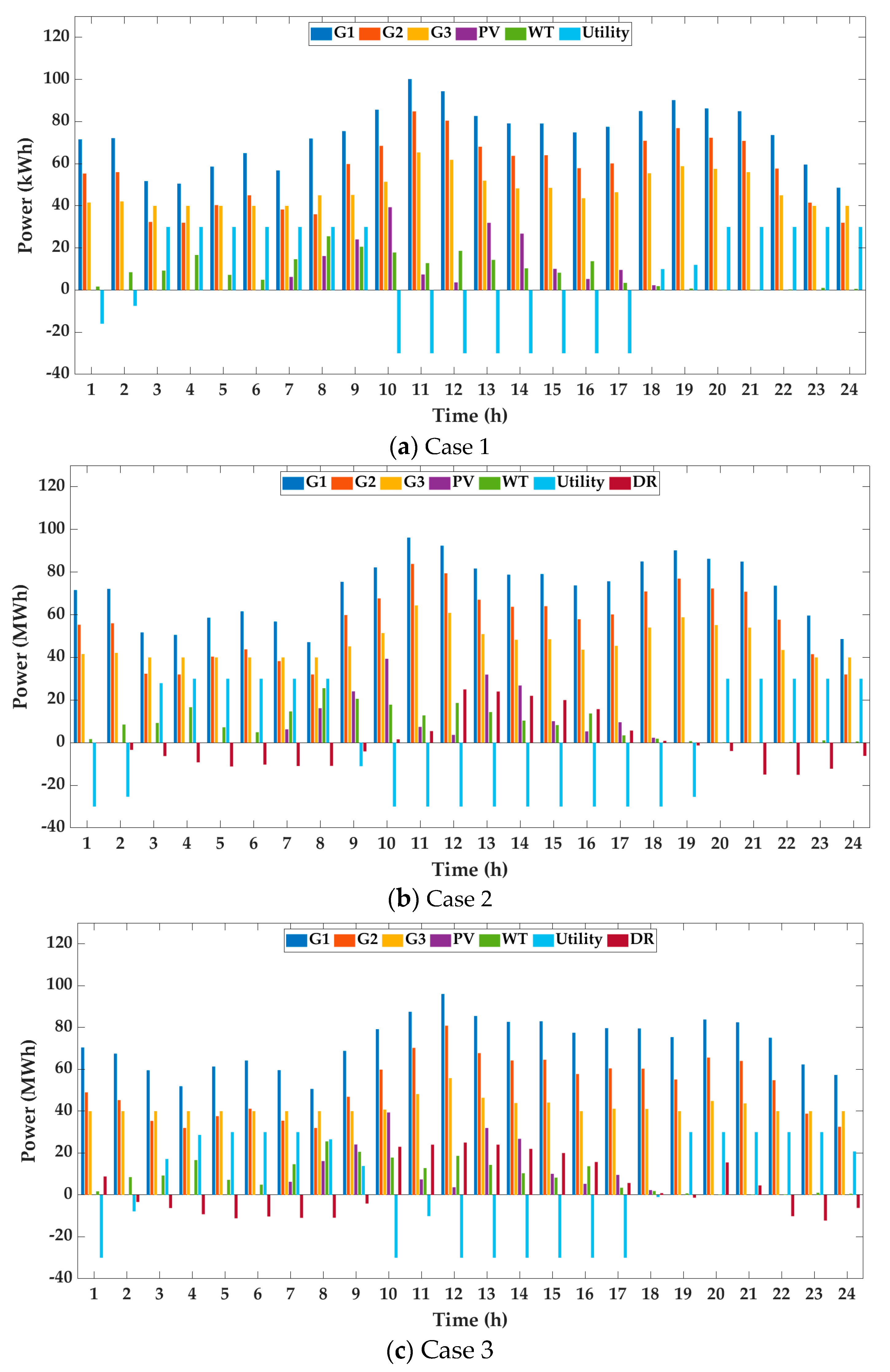
This paper proposed a CEED approach with the EBDR program by using the WU-ABC algorithm. The objective function was constructed in consideration of generation costs and pollutant emission. The emission function took the emitted quantities of CO₂, SOx, and NOx, into account and converts their sum into operation costs through unit conversion, using a penalty factor. To meet the maximum emission constraint considered in addition to the CEED in our work, the EBDR program was proposed to balance economics and environmental issues. The EBDR program is based on the concept of elasticity, and the participation volume changes depending on the violation of emission constraints. To solve the multiobjective optimization problem, we proposed the use of the WU-ABC algorithm, a combination of the weighting update method and the conventional ABC algorithm. To demonstrate the effectiveness of the proposed CEED approach, simulations were conducted on the modified grid-connected MG system. Three cases were considered depending on the maximum emission constraint and the application of a DR program. The proposed approach was able to reduce operation costs compared to the conventional solution without DR program. Furthermore, it was easy to satisfy the maximum emission constraints by updating the penalty factor. In summary, the use of the EBDR program reduced operation costs and pollutant emissions, and the maximum emission constraints were satisfied through the WU-ABC algorithm. Although operation costs were slightly increased compared to that of a conventional economic DR, an emission violation fee was not imposed. In addition, the performance test results indicated that the WU-ABC algorithm outperformed other algorithms in terms of cost and CPU time. Therefore, the proposed CEED approach can assist MGOs in optimizing MG operations under environmental constraints. Our future work will be under way to focus on solving the sensitivity problem in MG when the consumers do not comply with the command of MGO in the CEED problem.

References

1. Zhou, X.; Ai, Q.; Yousif, M. Two kinds of decentralized robust economic dispatch framework combined distribution network and multi-microgrids. Appl. Energy 2019, 253, 113588. [Google Scholar] [CrossRef]
2. Huijun, L.; Yungang, L.; Fengzhong, L.; Yanjun, S. A multiobjective hybrid bat algorithm for combined economic/emission dispatch. Int. J. Electr. Power Energy Syst. 2018, 101, 103–115. [Google Scholar]
3. Ghorab, M. Energy hubs optimization for smart energy network system to minimize economic and environmental impact at Canadian community. Appl. Therm. Eng. 2019, 151, 214–230. [Google Scholar] [CrossRef]
4. Ioanna, P.; Voula, P.K. The impact of carbon emission fees on passenger demand and air fares: Game theoretic approach. J. Air Transp. Manag. 2016, 55, 41–51. [Google Scholar]
5. Hossein, N.; Seyed-Ehsan, R.; Ali, A.; Ehsan, N.; Mehdi, F.; Mohammad, H.A.; Mohammad, R.N. A multi-objective framework for multi-area economic emission dispatch. Energy 2018, 154, 126–142. [Google Scholar]
6. Dhillon, J.S.; Parti, S.C.; Kothari, D.P. Stochastic economic emission load dispatch. Electr. Power Syst. Res. 1993, 26, 179–186. [Google Scholar] [CrossRef]
7. Kularni, P.S.; Kothari, A.G.; Kothari, D.P. Combined economic and emission dispatch using improved backpropagation neural network. Electr. Mach. 2000, 28, 31–44. [Google Scholar]
8. Majid, M.; Sayyad, N.; Kazem, Z. A cost-emission framework for hub energy system under demand response program. Energy 2017, 134, 157–166. [Google Scholar] [CrossRef]
9. Tong, X.; Hongyu, L.; Zhongfu, T.; Liwei, J. Coordinated energy management for micro energy systems considering carbon emissions using multi-objective optimization. Energies 2019, 12, 4414. [Google Scholar]
10. Albadi, M.H.; El-saadany, E.F. A summary of demand response in electricity market. Electr. Power Syst. Res. 2008, 78, 1989–1996. [Google Scholar] [CrossRef]
11. Kim, H.J.; Kim, M.K. Multi-Objective Based optimal energy management of grid-connected microgrid considering advanced demand response. Energies 2019, 12, 4142. [Google Scholar] [CrossRef] [Green Version]
12. Che, L.; Zhang, X.; Shahidehpour, M.; Alabdulwahab, A.; Abusorrah, A. Optimal interconnection planning of community microgrids with renewable energy sources. IEEE Trans. Smart Grid 2017, 8, 1054–1063. [Google Scholar] [CrossRef]
13. Nwulu, N.I.; Xia, X. Optimal dispatch for microgrid incorporating renewables and demand response. Renew. Energy 2017, 101, 16–28. [Google Scholar] [CrossRef]
14. El-keib, A.A.; Ma, H.; Hart, J.L. Environmentally constrained economic dispatch using a lagrangian relaxation method. IEEE Trans. Power Syst. 1994, 9, 1723–1729. [Google Scholar] [CrossRef]
15. Basu, A.K.; Bhattacharya, A.; Chowdhury, S. Planned scheduling for economic power sharing in a CHP-based micro-grid. IEEE Trans. Power Syst. 2012, 27, 30–38. [Google Scholar] [CrossRef]
16. Moghaddam, A.A.; Seifi, A.; Niknam, T.; Alizadeh Pahlavani, M.R. Multi-objective operation management of a renewable MG (micro-grid) with back-up micro turbine/fuel cell/battery hybrid power source. Energy 2011, 36, 6490–6507. [Google Scholar] [CrossRef]
17. Ghasemi, M.; Aghaei, J.; Akbari, E.; Ghavidel, S.; Li, L. A differential evolution particle swarm optimizer for various types of multi-area economic dispatch problems. Energy 2016, 107, 182–195. [Google Scholar] [CrossRef] [Green Version]
18. Jacob Rahlend, I.; Veeravalli, S.; Sailaja, K.; Sudheera, B.; Kothari, D.P. Comparison of AI techniques to solve combined economic emission dispatch problem with line flow constraints. Int J. Electr. Power Energy Syst. 2010, 32, 592–598. [Google Scholar] [CrossRef]
19. Aghajani, G.R.; Shayanfar, H.A.; Sshayeghi, H. Presenting a multi-objective generation scheduling model for pricing demand response rate in micro-grid energy management. Energy Convers. Manag. 2015, 106, 308–321. [Google Scholar] [CrossRef]
20. Nojavan, S.; Majidi, M.; Zare, K. Optimal scheduling of heating and power hubs under economic and environment issues in the presence of peak load management. Energy 2018, 156, 34–44. [Google Scholar] [CrossRef]
21. Nwulu, N.; Xia, X. Multi-objective dynamic economic emission dispatch of electric power generation integrated with game theory based demand response programs. Energy Convers. Manag. 2015, 89, 963–974. [Google Scholar] [CrossRef]
22. Behrangrad, M.; Sugihara, H.; Funaki, T. Effect of optimal spinning reserve requirement on system pollution emission considering reserve supplying demand response in the electricity market. Appl. Energy 2011, 88, 2548–2558. [Google Scholar] [CrossRef]
23. Parvania, M.; Fotuhi-Firuzabad, M. Demand response scheduling by stochastic SCUC. IEEE Trans. Smart Grid 2010, 1, 89–98. [Google Scholar] [CrossRef]
24. Abdelaziz, A.Y.; Ali, E.S.; Abd Elazim, S.M. Combined economic and emission dispatch solution using flower pollination algorithm. Int. J. Electr. Power Energy Syst. 2016, 80, 264–274. [Google Scholar] [CrossRef]
25. Dey, B.; Roy, S.K.; Bhattacharyya, B. Solving multi-objective economic emission dispatch of a renewable integrated microgrid using latest bio-inspired algorithms. Eng. Sci. Technol. Int. J. 2019, 22, 55–66. [Google Scholar] [CrossRef]
26. Guvenc, U.; Sonmez, S.; Duman, S.; Yorukeren, N. Combined economic and emission dispatch solution using gravitational search algorithm. Sci. Iran. 2012, 19, 1754–1762. [Google Scholar] [CrossRef] [Green Version]
27. Koltsaklis, N.E.; Giannakakis, M.; Georgiadis, M.C. Optimal energy planning and scheduling of microgrids. Chem. Eng. Res. Des. 2018, 131, 318–332. [Google Scholar] [CrossRef]
28. Mengelkamp, E.; Gärttner, J.; Rock, K.; Kessler, S.; Orsini, L.; Weinhardt, C. Designing microgrid energy markets: A case study: The Brooklyn Microgrid. Appl. Energy 2018, 210, 870–880. [Google Scholar] [CrossRef]
29. Lu, X.; Liu, Z.; Ma, L.; Wang, L.; Zhou, K.; Feng, N. A robust optimization approach for optimal load dispatch of community energy hub. Appl. Energy 2020, 259, 114195. [Google Scholar] [CrossRef]
30. Chiang, C.L. Improved genetic algorithm for power economic dispatch of units with valve-point effects and multiple fuels. IEEE Trans. Power Syst. 2005, 20, 1690–1699. [Google Scholar] [CrossRef]
31. Sampaio, P.G.V.; Gonzalez, M.O.A. Photovoltaic solar energy: Conceptual framework. Renew. Sustain. Energy Rev. 2017, 74, 590–601. [Google Scholar] [CrossRef]
32. Augustine, N.; Suresh, S.; Moghe, P.; Sheikh, K. Economic dispatch for a microgrid considering renewable energy cost functions. In Proceedings of the IEEE PES Innovative Smart Grid Technologies (ISGT), Washington, DC, USA, 16–20 January 2012; pp. 1–7. [Google Scholar]
33. Devi, A.L.; Krishna, O.V. Combined economic and emission dispatch using evolutionary algorithms-a case study. ARPN J. Eng. Appl. Sci. 2008, 3, 28–35. [Google Scholar]
34. Moghaddam, M.P.; Abdollahi, A.; Rashidinehad, M. Flexible demand response programs modeling in competitive electricity markets. Appl. Energy 2011, 88, 3257–3269. [Google Scholar] [CrossRef]
35. Shahryari, E.; Shayeghi, H.; Mohammadi-Ivatloo, B.; Moradzadeh, M. An improved incentive-based demand response program in day-ahead and intra-day electricity markets. Energy 2018, 155, 205–214. [Google Scholar] [CrossRef]
36. Secui, D.C. A new modified artificial bee colony algorithm for the economic dispatch problem. Energy Convers. Manag. 2015, 89, 43–62. [Google Scholar] [CrossRef]
37. Paliwal, N.K.; Singh, A.K.; Singh, N.K. Energy scheduling optimisation of an islanded microgrid via artificial bee colony guided by global best, personal best and asynchronous scaling factors. Int. J. Sustain. Energy 2020, 39, 539–555. [Google Scholar] [CrossRef]
38. Rezaee, J.A. Dynamic environmental-economic load dispatch in grid-connected microgrids with demand response programs considering the uncertainties of demand, renewable generation and market price. Int. J. Numer. Model. Electron. Netw. Devices Fields 2020, e2798. [Google Scholar] [CrossRef]
39. Hafstead, M. Projected CO2 Emissions Reductions under the American Opportunity Carbon Fee Act of 2017. Resources for the Future Issue Brief. 2017, 17-09. Available online: https://www.rff.org/ (accessed on 1 November 2020).
40. Hussain, S.; Al-Hitmi, M.; Khaliq, S.; Hussain, A.; Asghar Saqib, M. Implementation and comparison of particle swarm optimization and genetic algorithm techniques in combined economic emission dispatch of an independent power Plant. Energies 2019, 12, 2037. [Google Scholar] [CrossRef] [Green Version]
41. Ryu, H.S.; Kim, M.K. Two-Stage Optimal Microgrid Operation with a Risk-Based Hybrid Demand Response Program Considering Uncertainty. Energies 2020, 13, 6052. [Google Scholar] [CrossRef]
Figure 1. Proposed grid-connected microgrid (MG) system.
Energies 13 06450 g001
Figure 2. Valve point effect.
Energies 13 06450 g002
Figure 4. Optimal hourly scheduling in the MG for each case.
Energies 13 06450 g004
Figure 5. Penalty factor update and emissions.
Energies 13 06450 g005