Application of the Motion Capture System to Estimate the Accuracy of a Wheeled Mobile Robot Localization  ^†

Abstract

The paper presents research on methods of a wheeled mobile robot localization using an optical motion capture system. The results of localization based on the model of forward kinematics and odometric measurements were compared. A pure pursuit controller was used to control the robot’s behaviour in the path following tasks. The paper describes a motion capture system based on infrared cameras, including the calibration method. In addition, a method for determining the accuracy of robot location using the motion capture system, based on the Hausdorff distance, was proposed. As a result of the research it was found that the Hausdorff distance is very useful in determining the accuracy of localization of wheeled robots, especially those described by differential drive kinematics.

1. Introduction

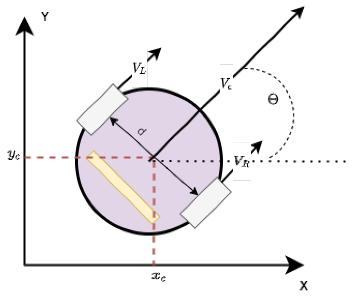
1.1. Wheeled Mobile Robots

In recent years, significant progress has been noted in the development of technologies that are related to control and communication of mobile robots, including wheeled mobile robots. Many new technological solutions supporting human labour are being created. Often these are works performed in difficult conditions or requiring a lot of physical effort, as well as works that people are not able to perform by themselves [1]. One of the fastest growing branches of robotics are mobile robots which have a great ability to move in land, air and water space [2]. Such robots can be controlled remotely by humans or can serve as autonomous units. Depending on the mobility system used, robots can be divided into: wheeled, walking, underwater and other [2]. Wheeled mobile robots are used in many areas of life, starting with simple household tasks such as cleaning and ending with specialised jobs such as working in a contaminated environment [3,4]. To improve the communication between robots and the possibilities of their autonomous work, new solutions are being developed. Robots are being equipped with the appropriate tools to enable them to carry out the tasks that are assigned to them. The implementation is supported by various locators such as GPS, vision systems and other additional sensors [5,6]. For effective movement in the environment it is necessary to create a map of the space surrounding the robot or use other methods, such as odometry [7]. They allow obtaining the robot position in a more efficient way [8,9]. The ongoing development of mobile robotics is related to the invention of new power supply systems, new materials, the increase in the computing power of electronic systems and the development of control systems which contributes to the creation of better projects applied in many areas of human life.

Wheeled mobile robots are constructed on the basis of various kinematics, including Ackermann’s (car-like) vehicles, bicycle kinematics and differential drive kinematics [7,10]. In this work the investigation of Quanser’s QBot2e wheeled mobile robot localization methods was presented. The motion of the QBot 2e can be described by the equations of differential drive kinematics. Forward kinematics is used to locate the robot in working space while inverse kinematics allows controling the robot and program its motion. The diagram of a mobile robot in the local reference frame is shown in Figure 1.

In Figure 1, the following kinematics parameters were assumed: $v_L$, $v_R$, m/s—linear speeds of the left and right wheel respectively, $v_c$, m/s—linear speed of the robot’s chassis, d, m—distance between wheels, $\Theta$, rad—angle of rotation of the chassis relative to the axis $OX$, $x_c,y_c$—coordinates of the chassis centre describing the robot’s position.

Taking into account the denotations in Figure 1, the following equations describing the robot’s motion can be derived [10,11,12]:

$$\begin{array}{cc}\hfill v_c& =\frac{v_R+v_L}{2},\hfill \\ \hfill {\omega }_c& =\frac{v_R-v_L}{d},\hfill \\ \hfill r_{ICC}& =d\frac{v_R+v_L}{2\left(v_R-V_L\right)},\hfill \end{array}$$

(1)

where: $r_{ICC}$ (m)—instantaneous radius of path curvature, ${\omega }_c=\dot{\Theta }$ (rad/s)—angular rate around robot’s axis of rotation.

Equation (1) refer to the description of movement relative to the local reference system (i.e., The system associated with the running platform). In practice, for example in a mapping of the surroundings, it is necessary to obtain a description in reference to the global coordinate system. In this case, the described model of simple kinematics takes the following form [10]:

$$\left[\begin{array}{c}\dot{x}\\ \dot{y}\\ \dot{\Theta }\end{array}\right]=\left[\begin{array}{c}\frac{1}{2}\left(v_R+v_L\right)cos\Theta \\ \frac{1}{2}\left(v_R+v_L\right)sin\Theta \\ \frac{1}{d}\left(v_R-v_L\right)\end{array}\right].$$

(2)

The inverse kinematics of the QBot 2e is expressed as follows:

$$\left[\begin{array}{c}{v}_R\\ v_L\end{array}\right]=\left[\begin{array}{c}{v}_c+\frac{1}{2}d{\omega }_c\\ v_c-\frac{1}{2}d{\omega }_c\end{array}\right].$$

(3)

In the research described in the later part of this work the models (2) and (3) were used to determine the position of the QBot 2e robot.

1.2. Dead Reckoning and Pure Pursuit Controller

One of the most important information necessary to control the movement of a mobile wheeled robot is information about its current location [8]. The procedure for obtaining the location based on the previous known position is called dead reckoning [9]. Odometric data recorded by rotary encoders connected to the wheels and/or IMU (inertial measurement unit) sensors installed on the robot (i.e., accelerometer and gyroscope) are used to determine the position of the robot [7]. Dead reckoning is used in many applications. For example, in [9] the authors compare three methods of mobile robot navigation. The paper describes studies of navigation algorithms with full use of IMU and kinematics constraints, with partial use of gyroscopic measurements and with the use of camera with depth measurement. In conclusion, the authors state that the correct calibration of the IMU sensor is crucial for the accuracy of navigation. In turn, the article [13] presents inertial navigation based on MEMS on dynamically positioned ships. The authors present an experimental validation and comparison of the possibility of calculating the localisation using two microelectron-mechanical IMU. Experimental validation was performed using two observers with non-linear characteristics, supported by the position reference systems and gyro-compasses, in a dynamic positioning operation conducted in the North Sea by a sea-going vessel.

In this work the accuracy of QBot 2 localization was compared with the use of pure kinematics model and odometric measurements. Further on, the results of these measurements were used for odometric localization of the robot, whereas the pose at time instant t, in global reference frame is obtained on the basis of integration of the Equation (2) in the range from 0 to t:

$$\left[\begin{array}{c}x\left(t\right)\\ y\left(t\right)\\ \Theta \left(t\right)\end{array}\right]={\int }_0^t\left[\begin{array}{c}\frac{1}{2}\left(v_R+v_L\right)cos\Theta \\ \frac{1}{2}\left(v_R+v_L\right)sin\Theta \\ \frac{1}{d}\left(v_R-v_L\right)\end{array}\right]dt.$$

(4)

This pose is then used to control the robot so that it moves along the planned path.

There are many metods to control the motion of the wheeled mobile robots used for the heading and speed control as well [7,10]. The robots can be controlled using, among others, classical control [10], optimal control [14,15], or geometric path tracking [16]. In this article, a pure pursuit algorithm [17] was used to control the movement of the QBot 2e robot. The pure pursuit algorithm allows the robot to follow the given path. The tracking is carried out by calculating the curvature of the vehicle’s path for each time. In the basic version of the method, the input data is a set of waypoints and a lookahead distance. This is the fixed distance between the current position of the robot and the current target point located on the path determined by the waypoints [16,17]. The curvature is calculated in such a way that each step of the algorithm allows the vehicle to travel from its current point to an instantaneous target point. As a result of the algorithm, the robot moves chasing the escaping instantaneous target point along the path. In this way, the vehicle reconstructs the curvature of the path with a certain accuracy. In practice, additional parameters characteristic for the type of kinematics (i.e., constraints) are introduced in the algorithm. In case of differential drive kinematics, these are the preset linear speed and maximum angular speed. An important issue related to the implementation of the above described method is the choice of the lookahead distance parameter. Let us define the tracking error as the shortest distance between the position of the robot and the path at the lookahead distance. In this case, the inverse of the lookahead distance represents the gain of the proportional controller. If the look ahead distance is too big (small gain), the tracking accuracy decreases. On the other hand, if the lookahead distance is too small (high gain), the robot’s movement shows oscillations around the given path. In the research presented in this work, the pure pursuit controller was used to control the robot in order to follow the given paths. The current pose, necessary to determine the robot’s movement in subsequent time instants, was obtained from the dead reckoning.

1.3. Motion Capture Systems and Path Similarity Measures

Optical motion capture is a technique that involves the recording of the position of people or objects in the real time. During capture, the position and orientation of objects in space is measured [18]. These systems are used in computer games and films. Motion capture is also used in military applications, robotics and medicine [18,19]. They can be divided into three groups: optical-passive, optical-active and video [18]. In the optical-passive case the system includes a set of infrared cameras and a set of reflective markers. Each tracked object is marked with markers which allows for clear object distinction. Objects tracked in an optical-active system have active markers (usually LEDs). Video systems use tracking software and detect objects based on the analysis of images in the visible band, recorded in real time. Modern systems, depending on the size of the markers, allow for a tracking accuracy of 1 mm.

In this work, the accuracy of location of the QBot 2e mobile robot controlled by a pure pursuit controller was evaluated. For this purpose it was necessary to define a quantitative measure of accuracy. In the study, the robot’s location determined with the use of motion capture system cameras was considered to be the reference location. To analyse the similarity between the trajectories of moving objects, different criteria can be used [20]. In particular, it is possible to use spatial-temporal measures [21] based on similarity analysis of time series [22] or metric and non-metric spatial criteria, such as e.g., Fréchet or Hausdorff’s measures [23]. The Fréchet distance is a non-metric measure. It takes into account the location and order of points along the curves determined by the shapes of analysed paths [23]. In this work the Hausdorff measure [24] was used to determine the similarity between the robot’s path estimated from odometric measurements or a model of kinematics and the reference path recorded by the motion capture system. The Hausdroff distance is a metric measure that measures how close the shape of the pathway A represented by a set of points of the working space (here: the plane) is to the shape of the path B. When calculating the distance for each point of the set (path) A, the distance to the nearest point of the set (path) B is determined. The next step is to calculate a maximum value from all these distances. Let it be given the complete metric space $(X,\rho )$ and the space of compact and non-empty subsets of space X denoted as $Z\left(X\right)$. Let A and B represent the space elements $Z\left(X\right)$ respectively. Additionally, by $x,y$ we will mark the space elements X, in such a way that $x\in A$ and $y\in B$. Taking the above notations it is possible to define the distance between the point $x\in A$ and the set of B, as:

$${\delta }_{xB}=inf\left\{d(x,y):y\in B\right\},$$

(5)

and between point $y\in B$ and the A set:

$${\delta }_{yA}=inf\left\{d(x,y):x\in A\right\}.$$

(6)

In addition, using Equations (5) and (6) it is possible to calculate the distance ${\delta }_{AB}$ between a A set and a B set and the interval ${\delta }_{BA}$ between a B set and a A set:

$${\delta }_{AB}=sup\left\{{\delta }_{xB}:x\in A\right\},{\delta }_{BA}=sup\left\{{\delta }_{yA}:y\in B\right\}.$$

(7)

Given (7), the Hausdorff metric can be defined as:

$$H_{AB}=max\left\{{\delta }_{AB},{\delta }_{BA}\right\}.$$

(8)

The measure $H_{AB}$ defined above has been used as a quantitative measure of the accuracy of the odometric localization of the QBot 2e mobile robot using a reference localization obtained from the motion capture system.

The remaining sections of the paper are organized as follows. In Section 2, the methodology of experimental investigations using Test stand for evaluating the control algorithms for mobile wheeled robots are described. In Section 3, the results of experiments conducted for two kinds of robot path are presented. Analysis of the results is shown in Section 4. Finally, Section 5 is a summary of our conclusions.

2. Materials and Methods

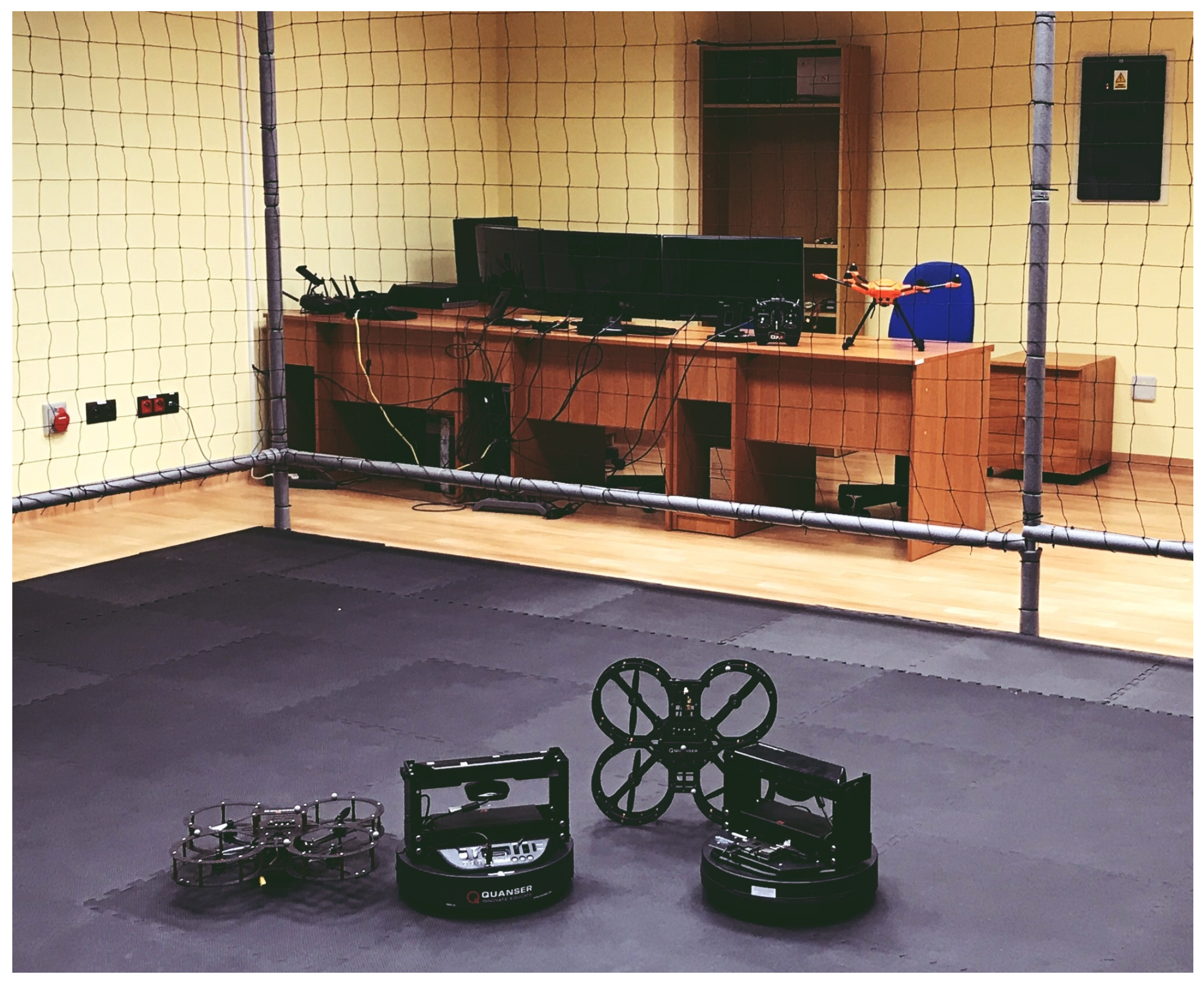
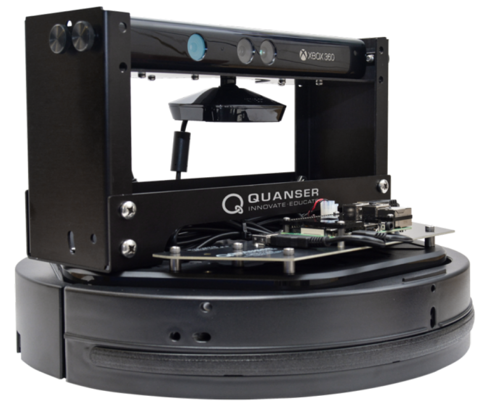
2.1. Test Stand for Evaluating the Control Algorithms for Mobile Wheeled Robots

The experimental research was carried out with the use of the Autonomous Vehicles Research Studio hardware and software kit provided by QUANSER, which enables testing of control algorithms for mobile robots (i.e., Laboratory of Intelligent Mobile Robots). The setup consists of four quadrocopters (QDrone), two wheeled robots (QBot 2e), eight tracking cameras (OptiTRACK Flex 13) and a ground control station [25,26]. The photo of the laboratory is presented in Figure 2.

The ground control station consists of a PC with the following parameters: Intel Core i7 with 32 GB of DDR4 RAM and software: Matlab 2018a, QUARC Real-Time Control Software 2018, Motive 2.0 and Visual Studio Community Compiler 2017. There are also three monitors, USB flight controller joystick, and the two-band WiFi router in the lab.

One of the elements of the environment is the QBot 2e mobile robot. It is an autonomous ground robot with an open architecture. It is built on Kobuki’s two-wheeled mobile platform. QBot 2e consists of two drive wheels with encoders mounted on a common axis. The distance between the left and right wheel is 0.235 m. The diameter of the vehicle is 0.35 m and its height (without additives) is 0.10 m with the Kinect sensor mounted up to 0.27 m. The platform can move with a maximum linear speed of 0.7 m/s. The robot uses a drive mechanism called a differential drive. Front and back wheels of the robot stabilize the platform without any movement impairment. Each drive wheel can be independently driven forward and backward. The movement of each wheel is measured by means of encoders (2578 counts per revolution) and the orientation of the robot or the yaw angle can be estimated by means of an integrated gyroscope embedded in an inertial measurement unit (MEMS IMU). QBot 2e has integrated impact bumpers (left, right and centre) and cliff sensors (left, right and centre). The robot is equipped with the Raspberry Pi 3 B+ on-board computer and integrated wireless LAN, which allows wireless connection between the test station and/or other vehicles. On te platform of the robot you will find the Microsoft Kinect vision system which allows you to process RGBD (Read-Green-Blue-Depth) data for various purposes, including visual inspection or 2D and 3D grid mapping. The QBot 2e cameras have a resolution of 640x480 pixels. The Kinect depth sensor uses infrared light and has a range from 0.5 m to 6 m [1]. The total weight of the robot is 3.82 kg. The QBot 2e robot is shown in Figure 3.

The working space is surrounded by a safety grid. The floor is lined with anti-slip panels. Total size of the working space is $5\times 5\times 2.5$ m. Inside the working space, under the ceiling, there are eight OptiTRACK Flex 13 cameras with resolution of 1280 × 1024, native frame rate 120 Hz, latency 8.3 ms and 3D and Accuracy ± 0.20 mm. Cameras are designed to work with passive reflective markers of 9 m in diameter and stock lens ${56}^{\circ }\times {46}^{\circ }$ FOV. The shutter default Speed is equal to 0.25 ms. Four cameras are placed in the corners, the other four in the middle of the sides. The cameras are used to track the position of mobile robots. This is achieved by means of dedicated software for this purpose—Motive 2.0. Tracking of mobile robots is possible by mounting special markers on each of them. The marker layout on a particular robot must be unique so that the software can identify the object.

In the software layer, the laboratory is equipped with a Matlab/Simulink computational environment, cooperating with Quanser QUARC hardware drivers. This enables the key functionalities required for research on multiple vehicles through a variety of configurable modules. In addition, it allows for the creation of high-level applications and reconfiguration of low-level processes supported by the manufacturer’s pre-built QUARC Simulink libraries. These applications can be expanded or created from scratch using only blocks or fragments of the previously mentioned blocks.

QUARC Real-Time Control Software 2018 generates real-time code directly from the drivers designed by Simulink and runs it in real time on a Windows real-time target or a real-time target on Linux installed on QBot 2e compute module. Due to the need for communication between the workstation and the robot, two models created in Simulink are often used. One of them called the Mission Server allows planning the path of the robot and the other one commonly called the Stabilizer is responsible for its completion. Each of the above mentioned models is running on a different system target. Mission Server on a Windows-based ground control station and Stabilizer on the Linux operating system. The models exchange data via the TCP IP protocol and a wireless router.

2.2. Methodology of Research

The following section describes the methodology of testing two algorithms of QBot 2e localization carried out on the described stand. Research was conducted in the following stages:

In the further part of this work, the methodology of research of two localization algorithms of QBot 2e

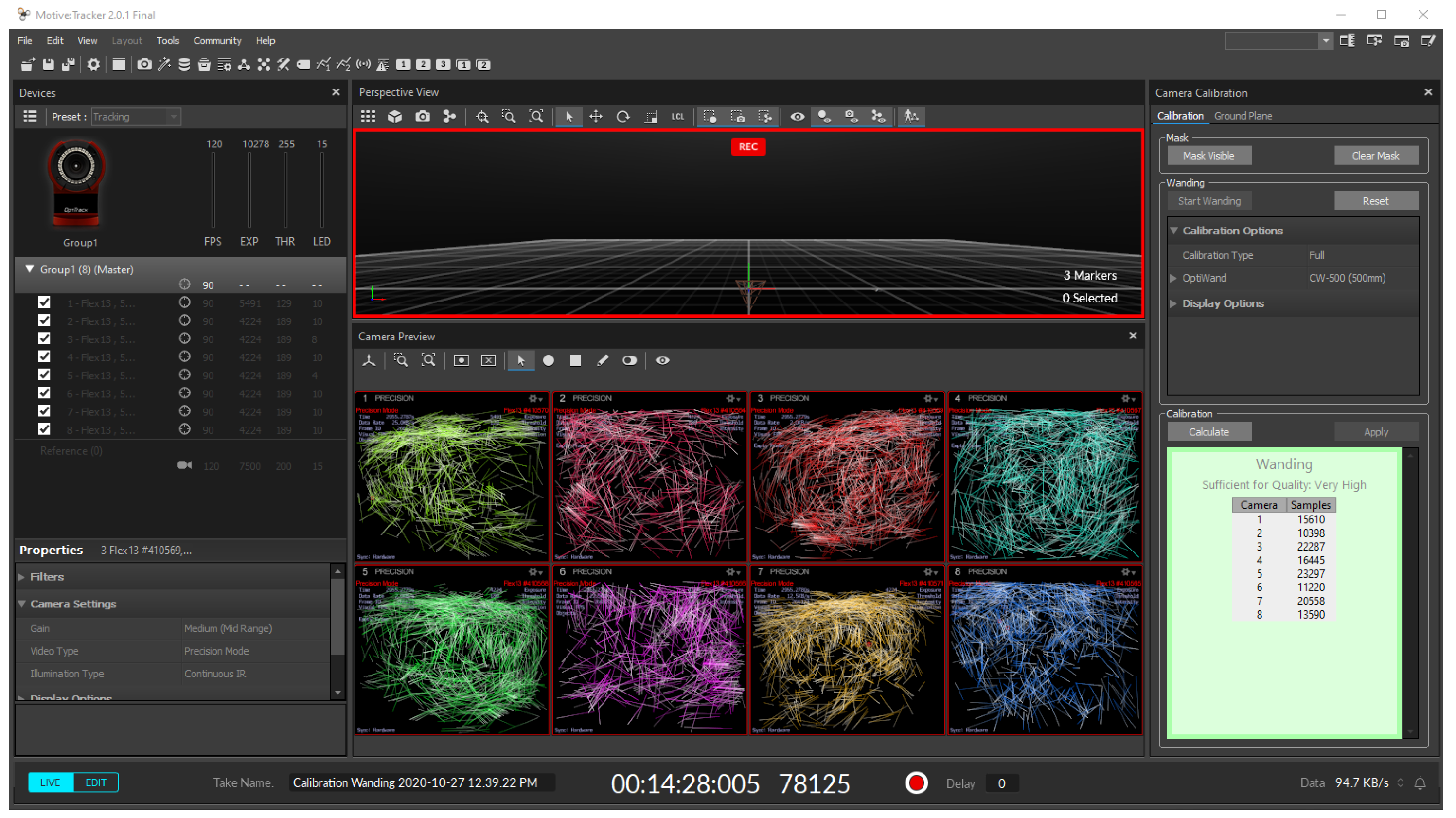
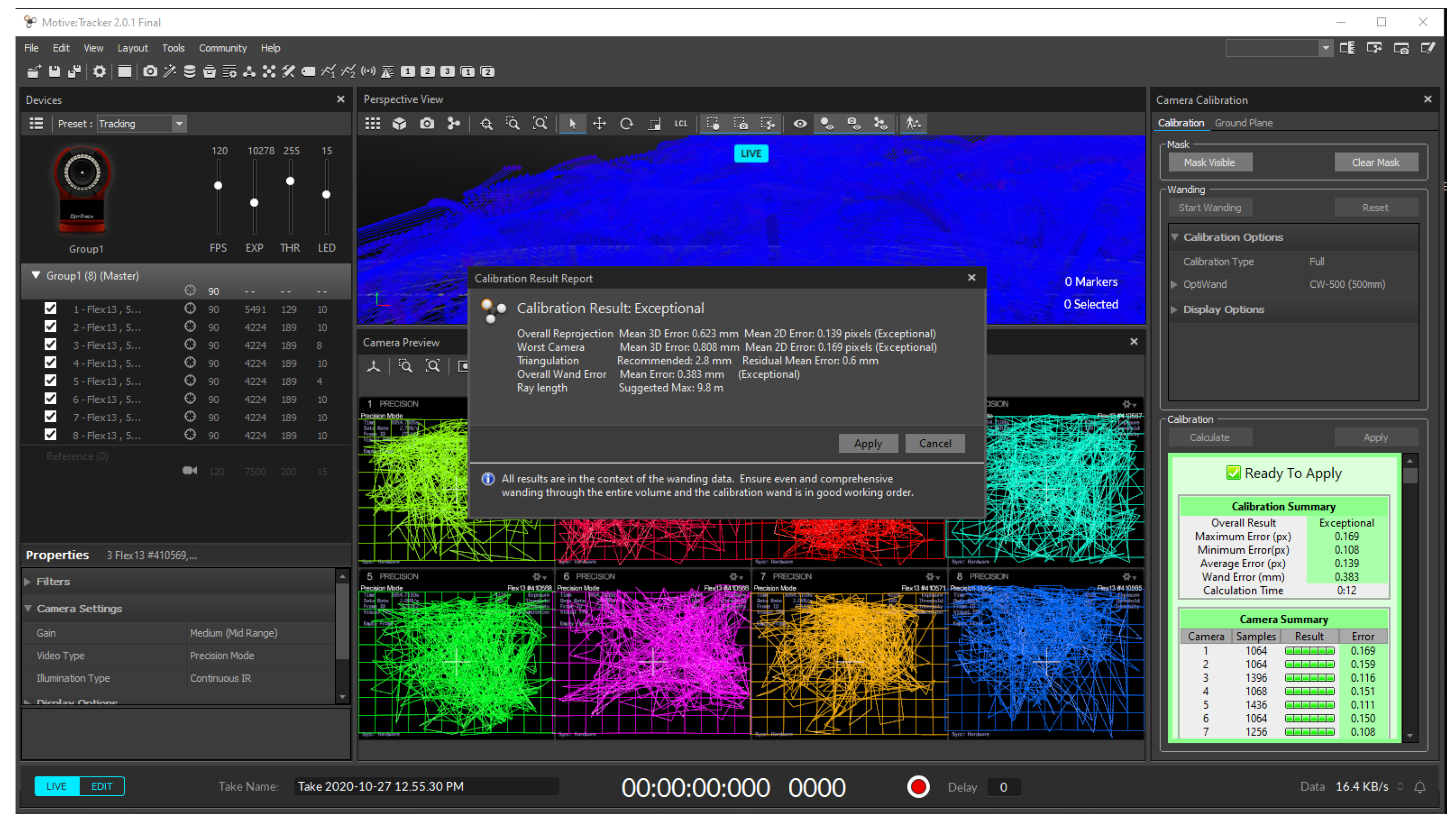
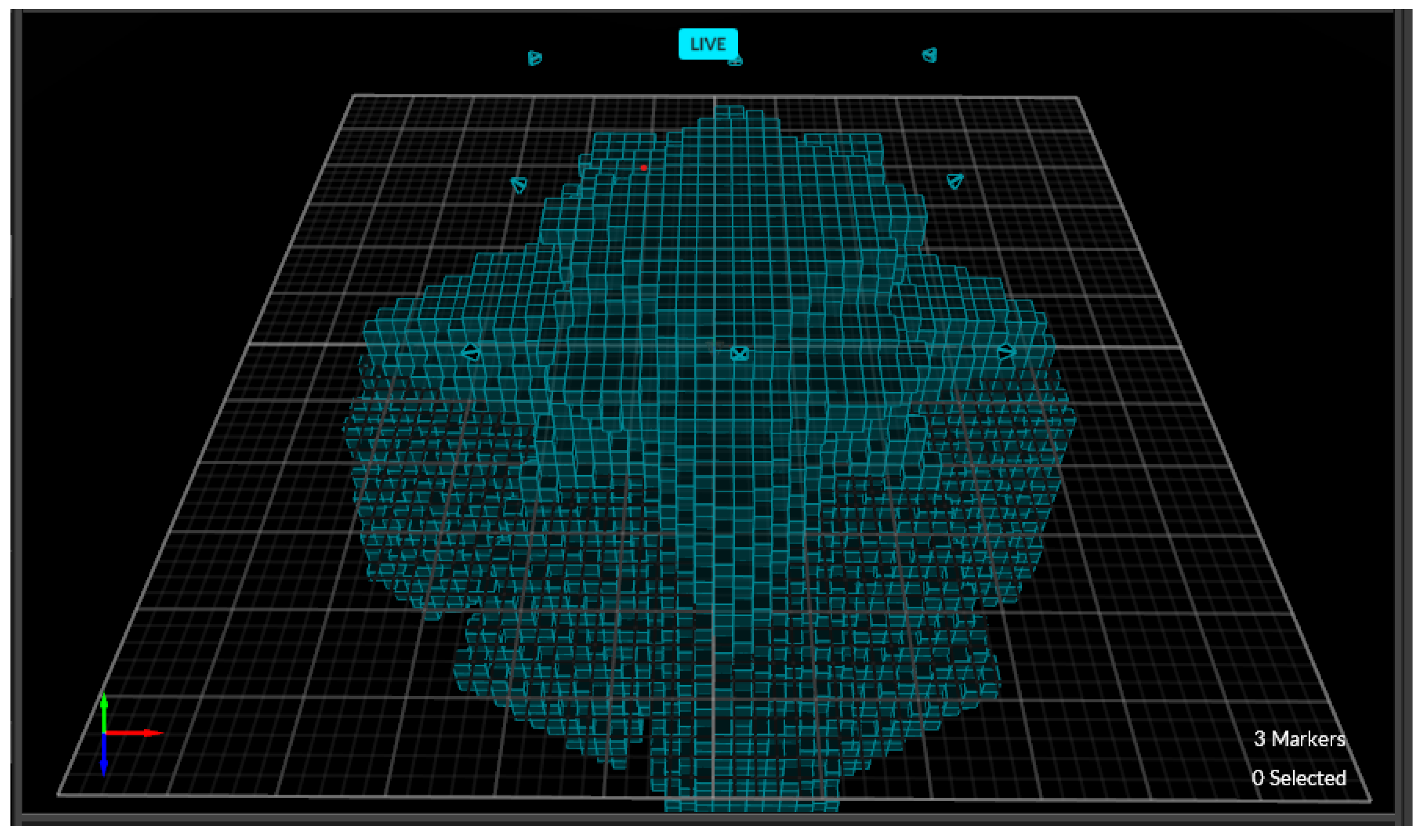
• Calibration of the OptiTRACK motion capture system;
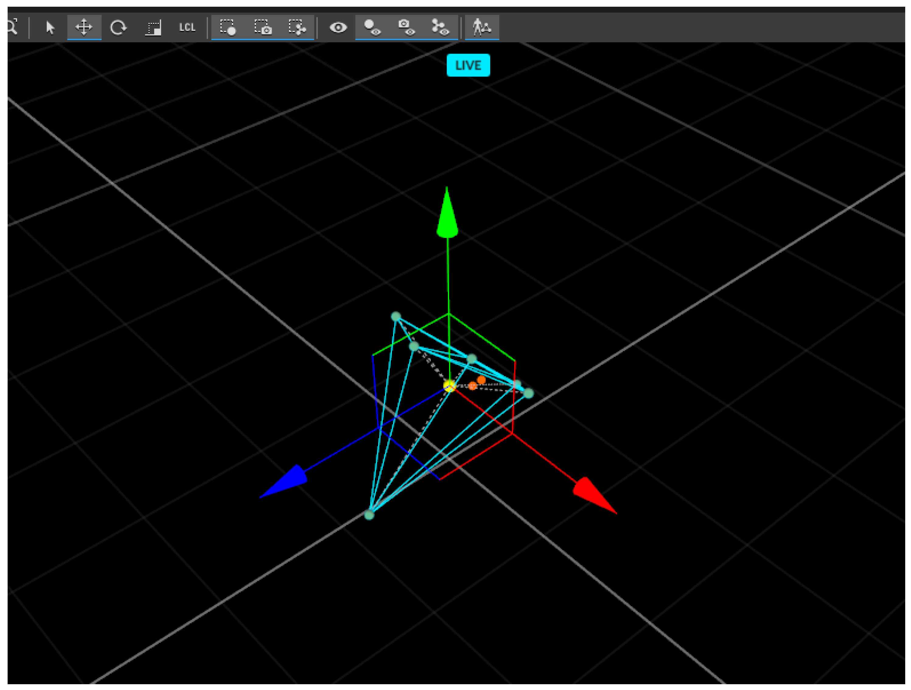
• Definition of geometric model of rigid body in Motive 2.0;
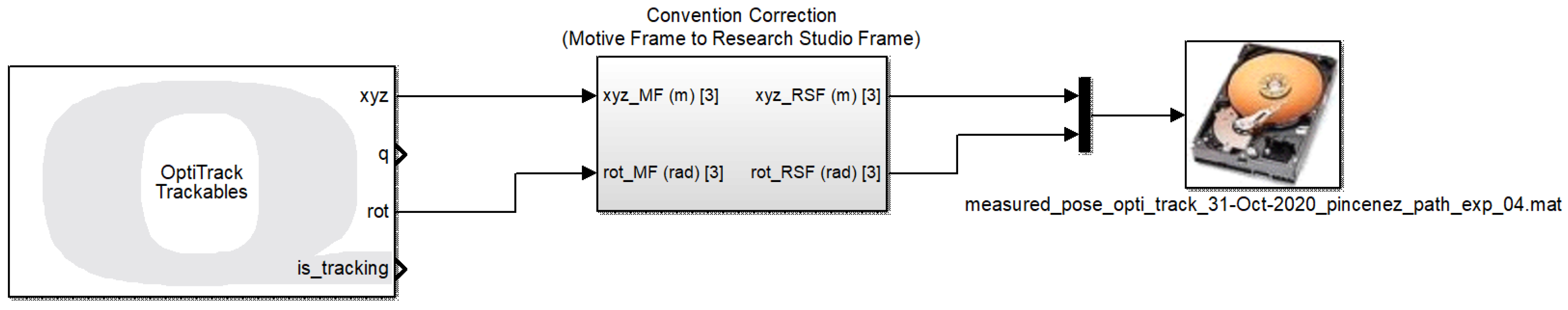
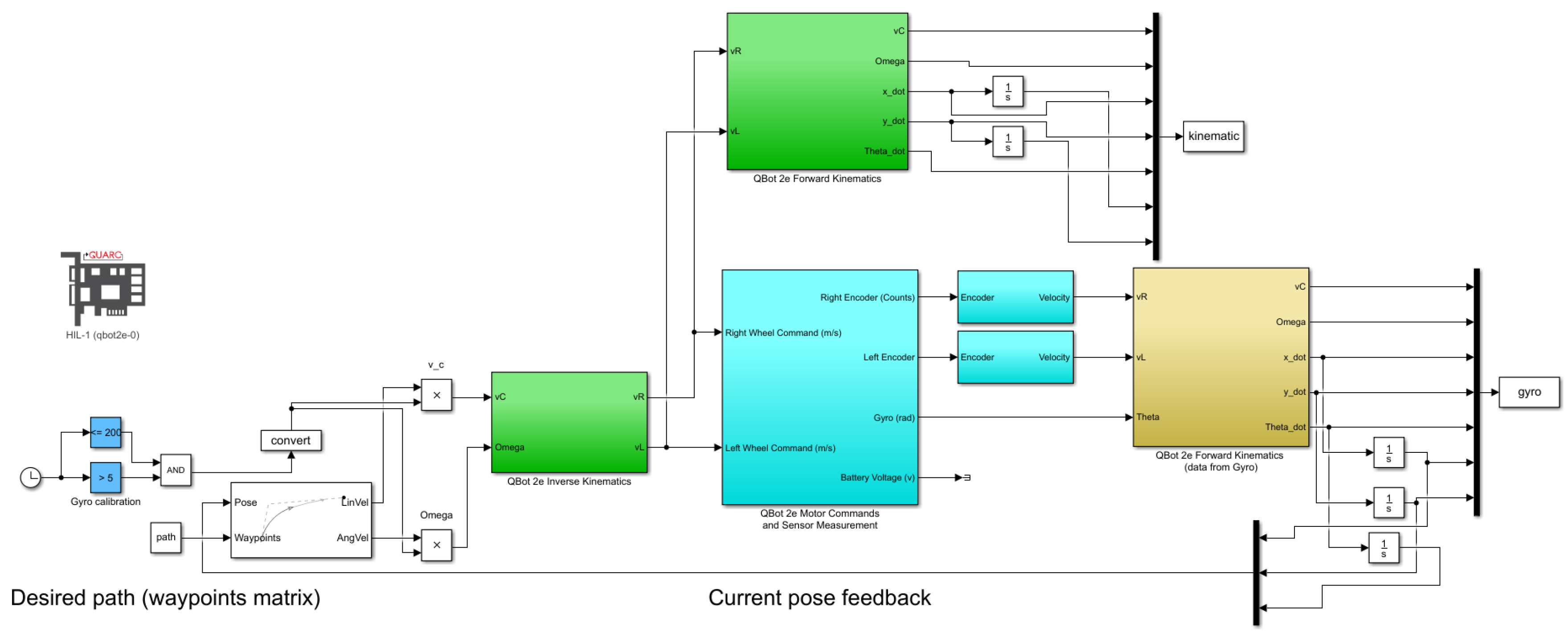
• Creation of a Simulink diagram allowing capturing the robot’s motion by OptiTRACK camera system;
• Programming the robot’s movement according to the assumed path in the Matlab/Simulink environment;
• Compile an i transmission of the simulation model to the target platform running in the real time target;
• Running the model on the target platform and hardware in the loop (HIL) simulation;
• Analysis of HIL results, including determination of Hausdorff measures for recorded tracks.

To properly track the objects moving in a working space, the OptiTRACK system needs to be calibrated. This process consists of the two following stages:

• Determining the relative position of the cameras inside the working space;
• Determining the position of cameras in relation to the ground (ground level calibration).

The first stage of calibration was carried out with a CW-500 calibration wand. The wand has appropriately positioned reflective markers. The size of the markers and their distances to each other are stored in Motive software, which operates the cameras. During the calibration process, the position of the markers during the wanding inside the working space was recorded. The recording was carried out using all eight cameras of the system to obtain a point marker cloud. Motive software then carried out calculations which resulted in the determination of the positions and positioning of the cameras or each other. The Figure 4 shows the screens of the Motive program after calibration. The screen of the Motive software after the point cloud calculations is presented in Figure 5.

In the second stage, the camera positions on the floor were determined using the calibration element CS-200. As before, the position of the markers located on the calibration element CS-200 was transferred from the cameras to the software. This was used to determine the position of the cameras and the floor. In addition, the capture volume was determined during the calibration process. The capture volume visualization screen is shown in Figure 6.

A calibration file was generated as a result of the calibration. This file is then loaded in a special Simulink diagram block. The block allows obtaining the current position of the robot being Tracked during the hardware in the loop simulation described later in this work. It should be emphasised that it is recommended to perform calibrations each time before starting the investigations on a given day. This is necessary due to changing environmental conditions, especially lighting conditions and temperature.

In the next stage of research, geometrical model of a rigid body representing QBot 2e robot was defined.

The geometric model of a rigid body is a set of points in a space interrelated in such a way that the distance between them does not change. Any physical objects not subject to deformation can be modeled as rigid bodies. Determination of the position of a rigid body is possible on the basis of knowledge of the position of at least three of its constituent particles and mutual distances between the particles. From a practical point of view, the centre of mass or the geometric centre of the body together with the orientation of the body is often used to determine the position of a rigid body.

During the research, six reflective markers were glued to the top of the robot, positioned asymmetrically. The markers were placed on the upper surface to ensure the best possible visibility for cameras installed above the workspace. The markers’ placement on the QBot 2e robot platform is shown in Figure 7.

Next, the rigid body was modeled in Motive. For this purpose the QBot 2e robot was positioned in the workspace. Then, on the basis of the set of points a rigid body model was created. The model of the created rigid body is depicted in Figure 8.

As a result of creating the rigid body model, a file containing information about its rigid body was obtained. This file was then used to track the robot’s path by algorithms prepared in Matlab environment using QUARC drivers. The registration of the robot’s movement in the Simulink environment was carried out using the PoseTracker.slx diagram presented in Figure 9.

The main element of the scheme is the OptiTRACK Trackables block, which requires Motive program files containing calibration data and a model of the rigid body to work properly.

For programming the robot’s motion a simulation model of the Simulink was used. The diagram is shown in Figure 10.

The robot’s movement has been programmed in such a way that it is possible to compare the location obtained using odometric data recorded in real time by the encoders connected to the robot’s wheels and the IMU sensor installed on the driving platform (Figure 10 blue block), with the results of simulation of the (2) and (3) models, (Figure 10 green block).

The experiments were carried out using the hardware in the loop (HIL) simulation method for two shapes of robot paths. The paths were given using a waypoints matrix. To control the robot, a pure pursuit path tracking algorithm was used. HIL simulations were carried out for four sets of test parameters including the set line speed ($v_c$), maximum angular speed (${\omega }_{max}$) and lookahead distance ($L_d$). Parameter values used in the simulation for path $P_1$ and $P_2$ are listed in

Table 1. The values of parameters used in the hardware in the loop simulation for $P_1$ path.

Simulation #	${\mathit{v}}_{\mathit{c}}$ (m/s)	${\mathit{\omega }}_{\mathit{max}}$ (rad/s)	${\mathit{L}}_{\mathit{d}}$ (m)
1	0.1	1.0	0.2
2	0.1	0.5	0.2
3	0.1	1.0	0.1
4	0.1	0.5	0.1

and

Table 2. The values of parameters used in the hardware in the loop simulation for $P_2$ path.

Simulation #	${\mathit{v}}_{\mathit{c}}$ (m/s)	${\mathit{\omega }}_{\mathit{max}}$ (rad/s)	${\mathit{L}}_{\mathit{d}}$ (m)
1	0.2	1.5	0.1
2	0.2	0.7	0.1
3	0.2	1.5	0.2
4	0.2	0.7	0.2

respectively.

During the execution of the specified paths, the data from encoders and the gyroscope were recorded in real time. Subsequently, the results of these measurements were used for odometric localization of the robot. Its current pose at the time instant t in the global reference frame was obtained from Equation (4).

The final stage of the study was the off-line analysis of the HIL simulation results. In the analysis the following parameters were determined:

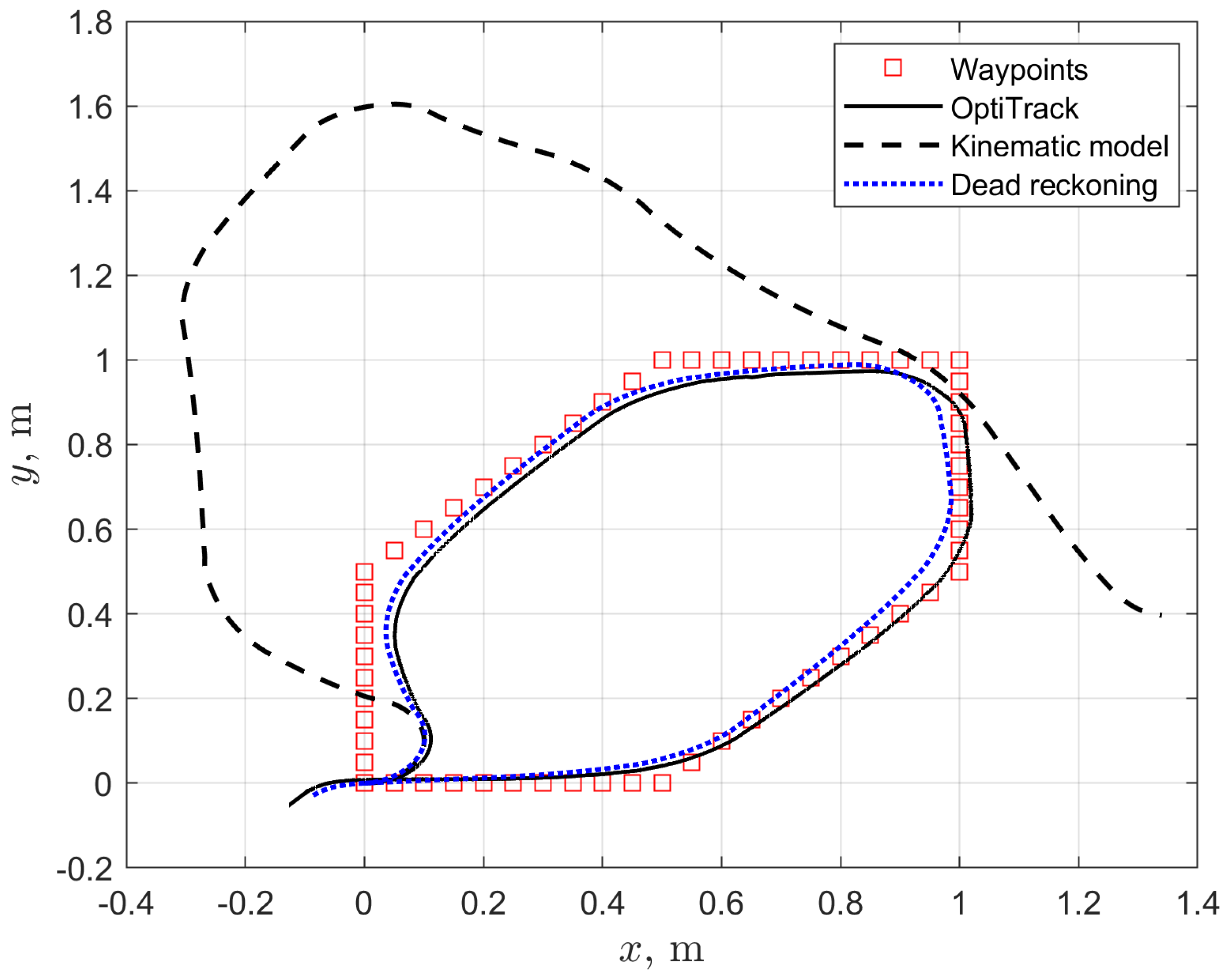
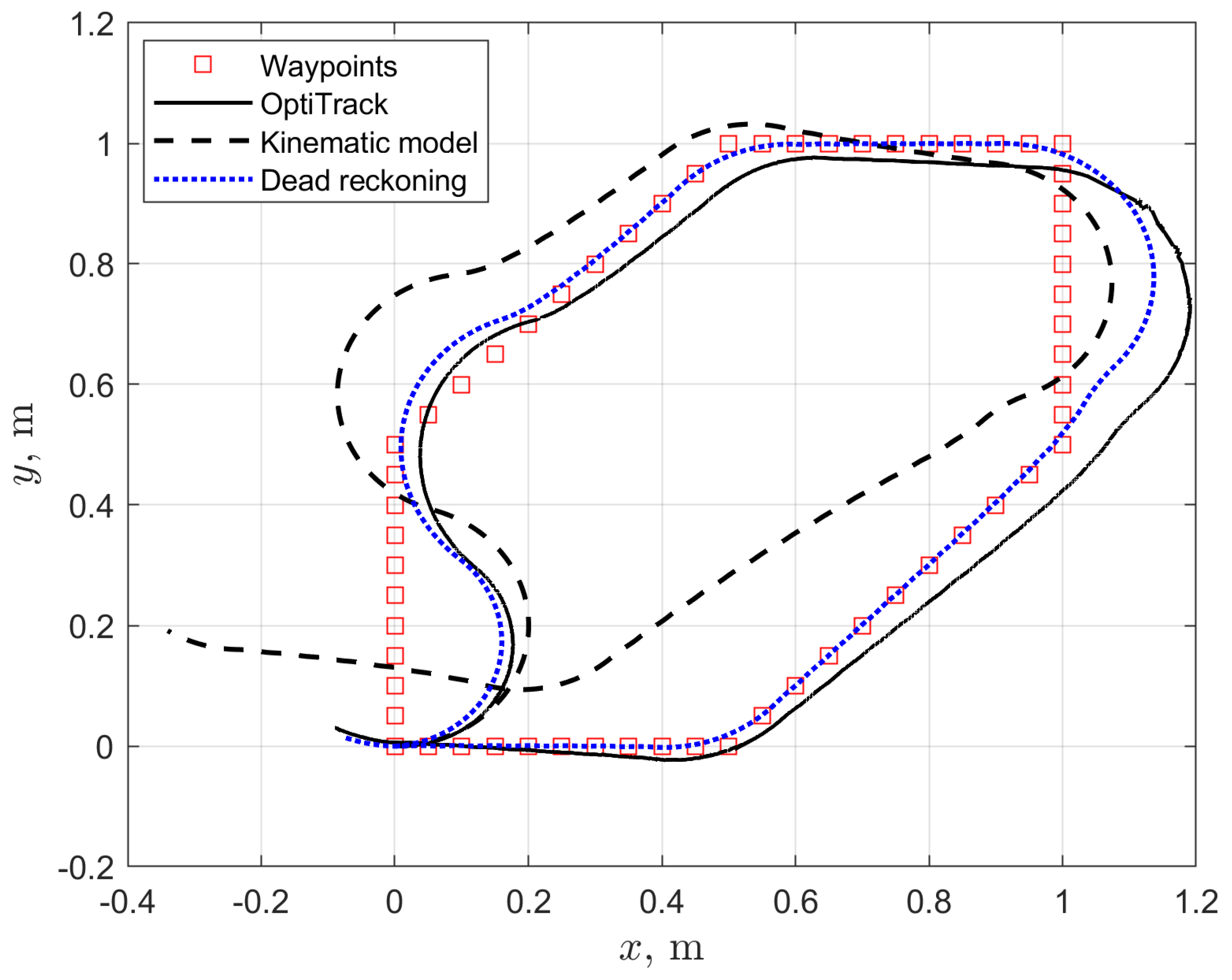
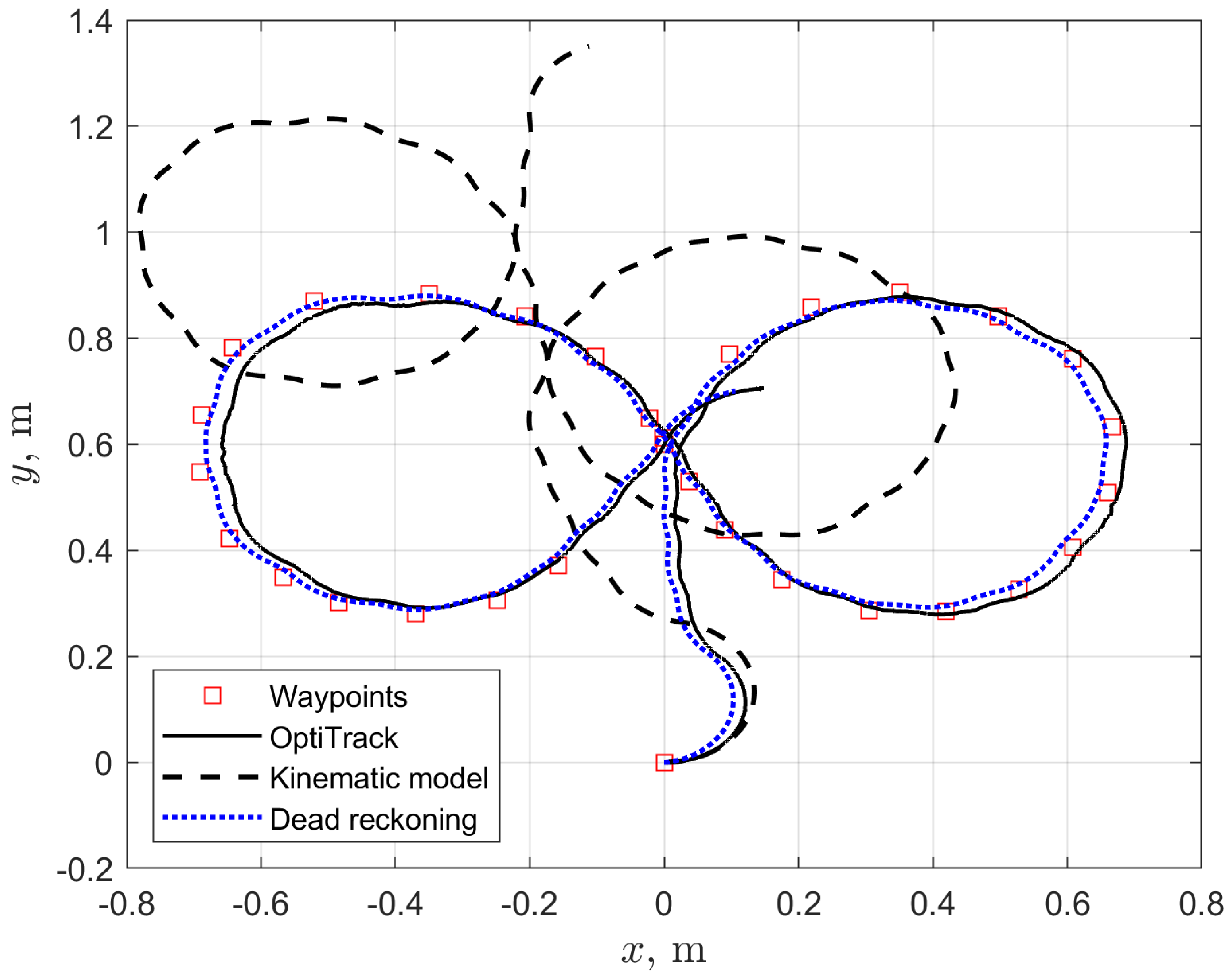
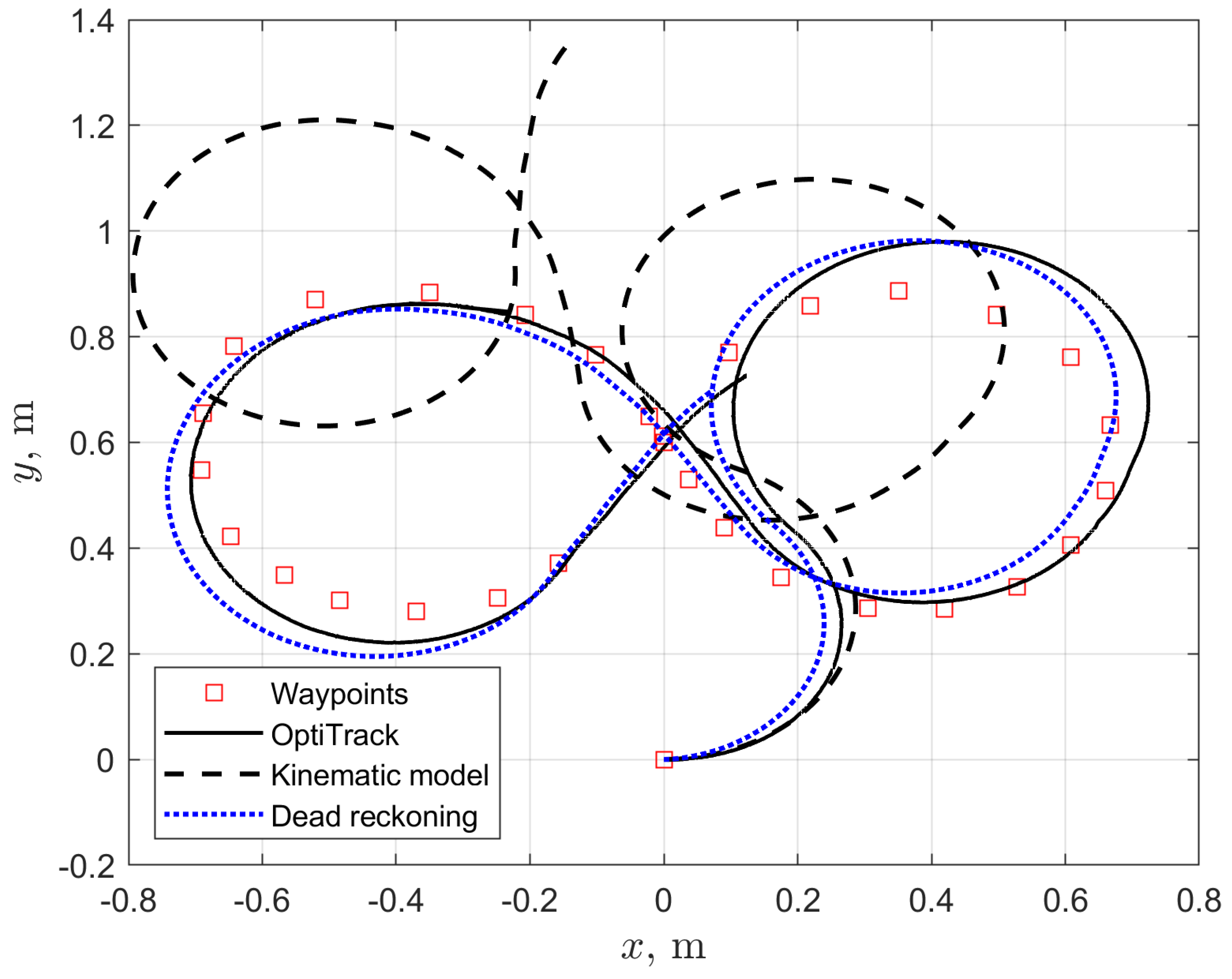
• The Hausdorff distance $H_{OO}$ between the path determined by the odometric localization and the reference path recorded by the OptiTRACK system
• The Hausdorff distance $H_{OK}$ between the path determined on the basis of the kinematics model and the reference path recorded by the OptiTRACK system
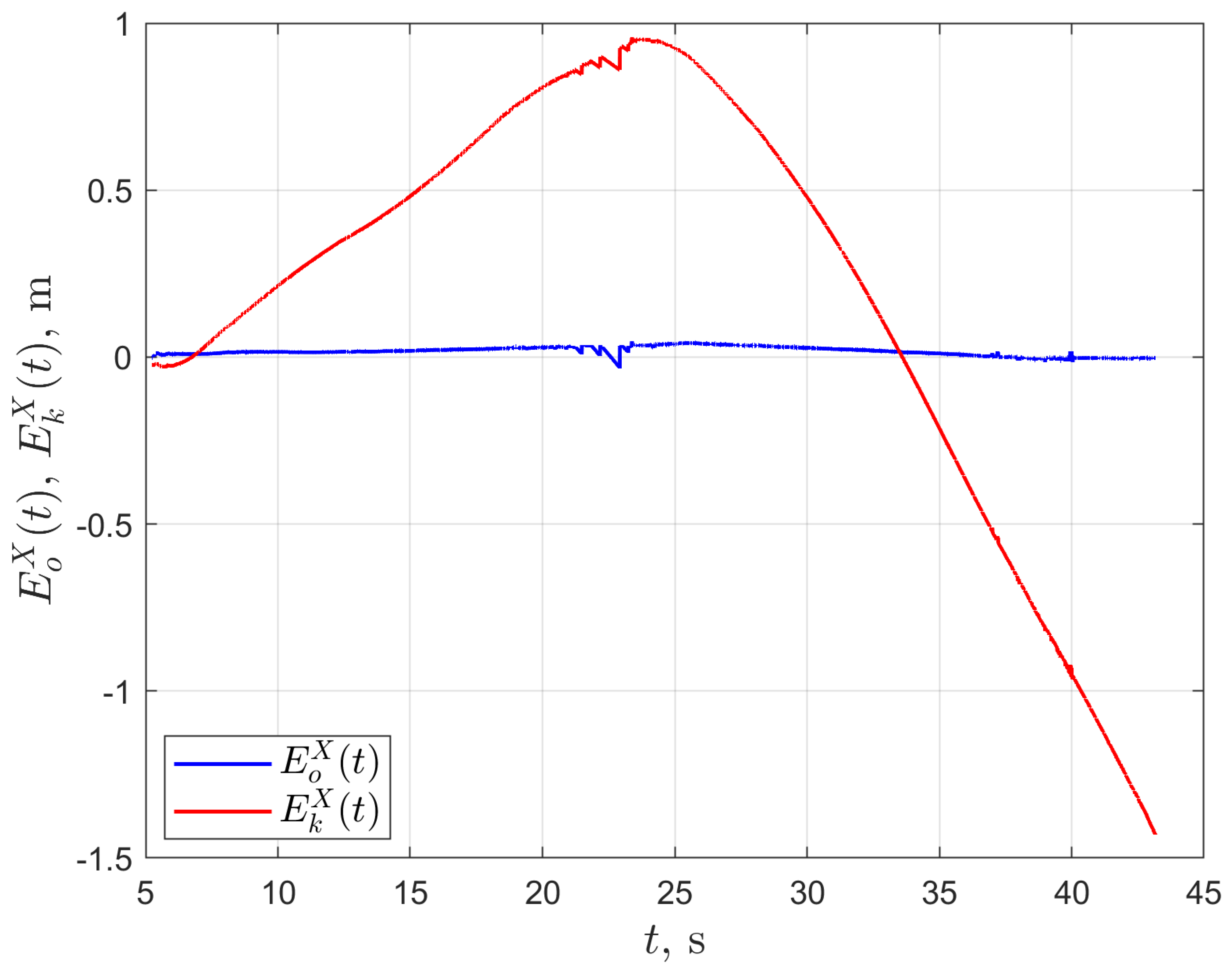
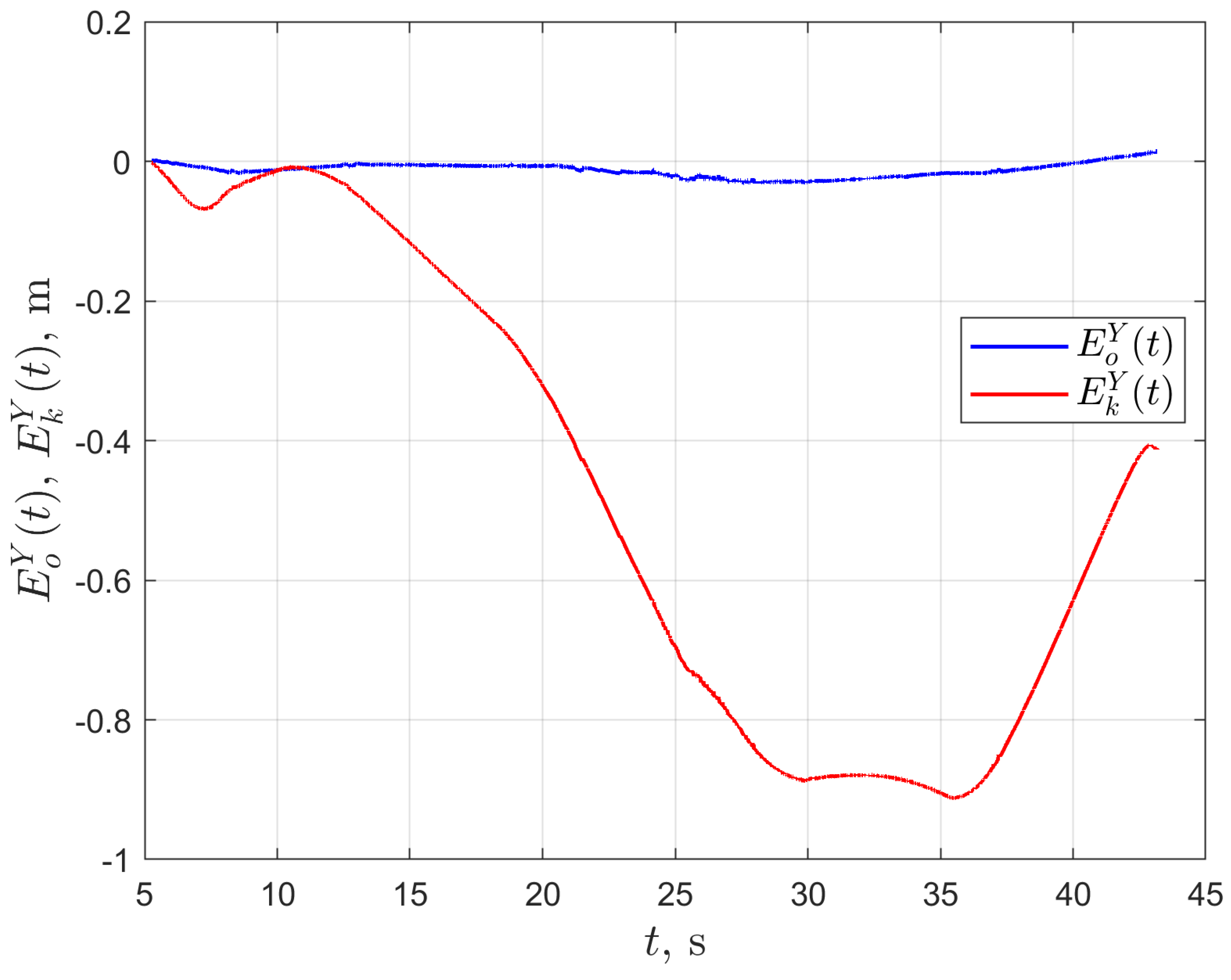
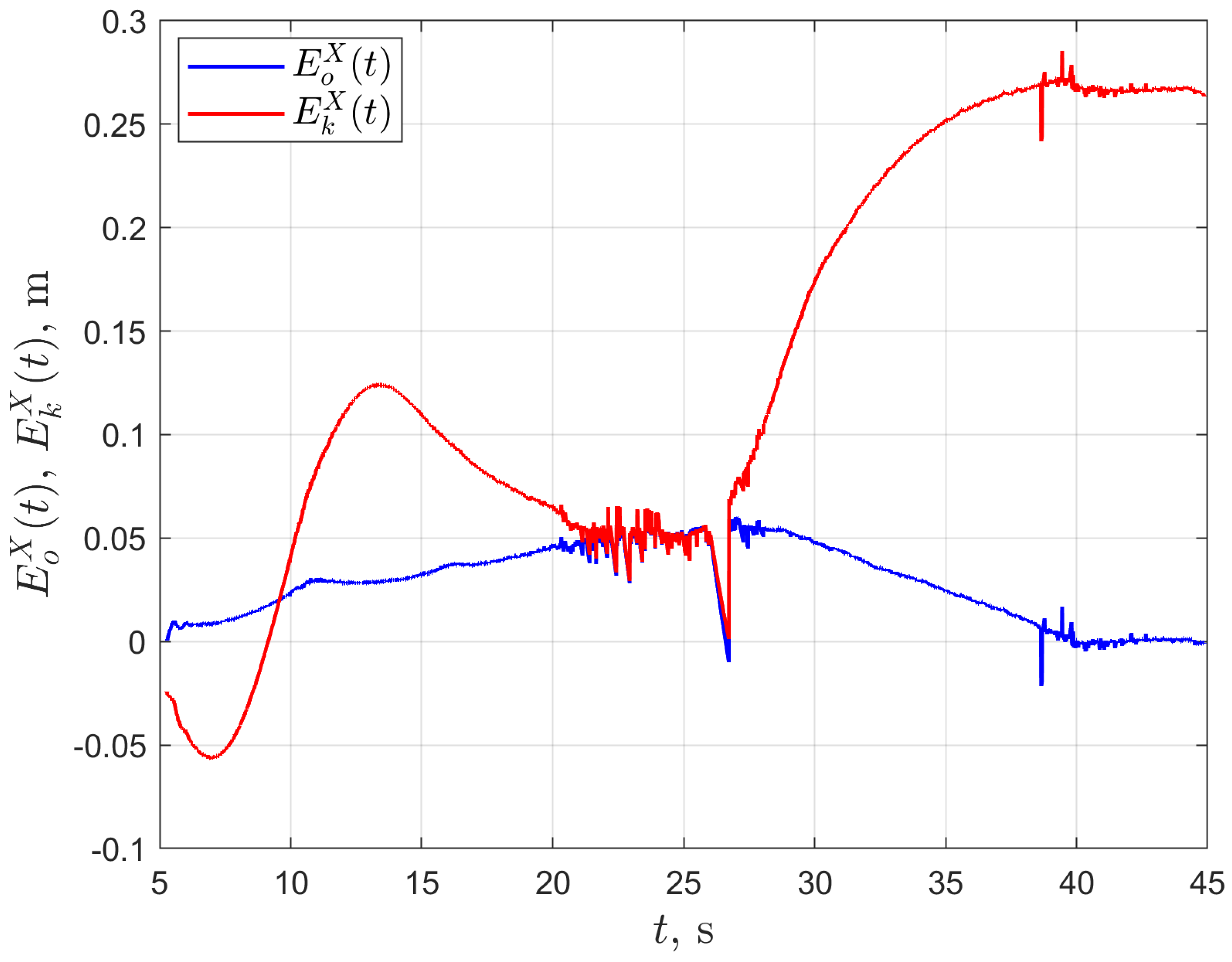
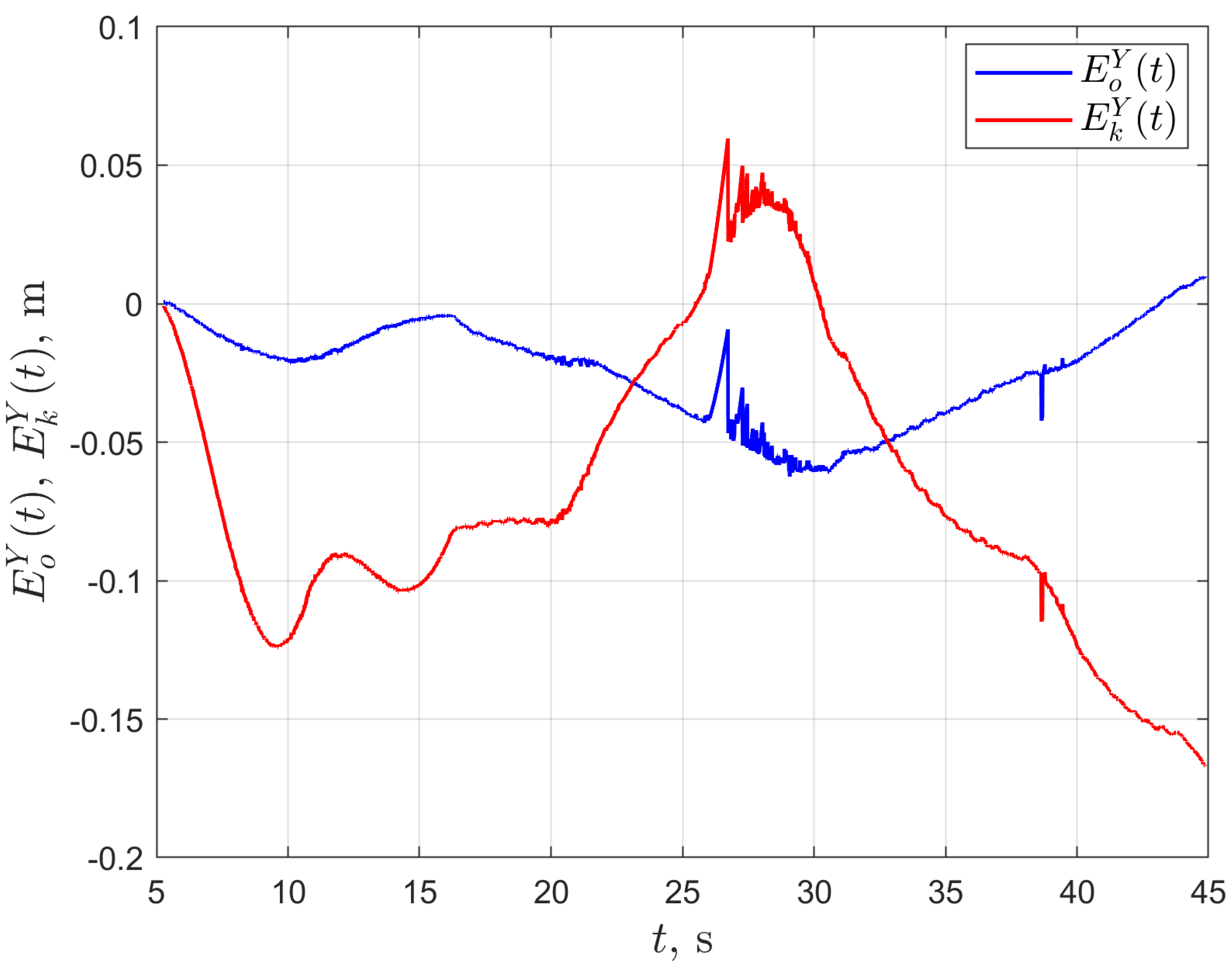
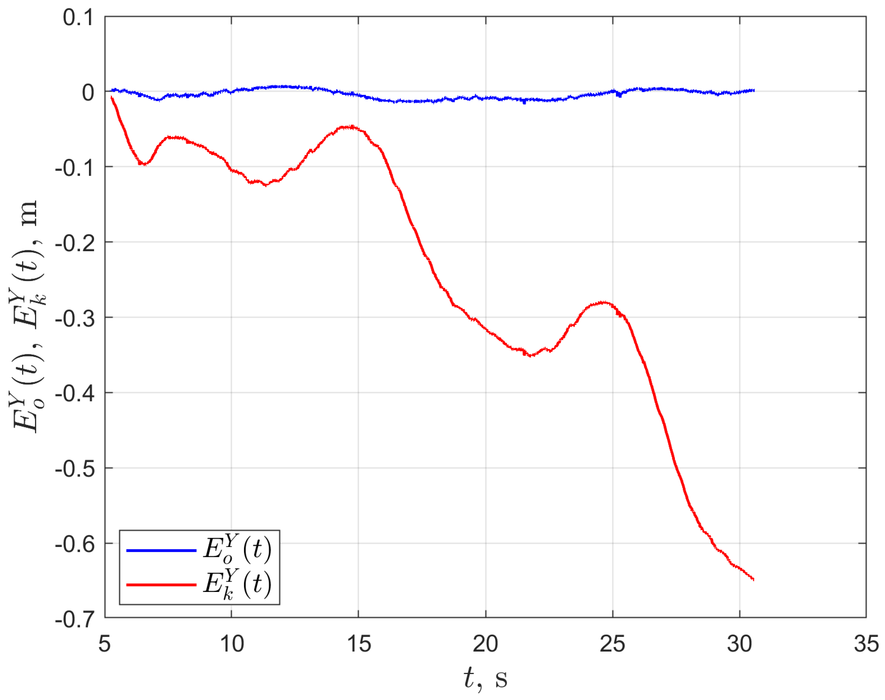
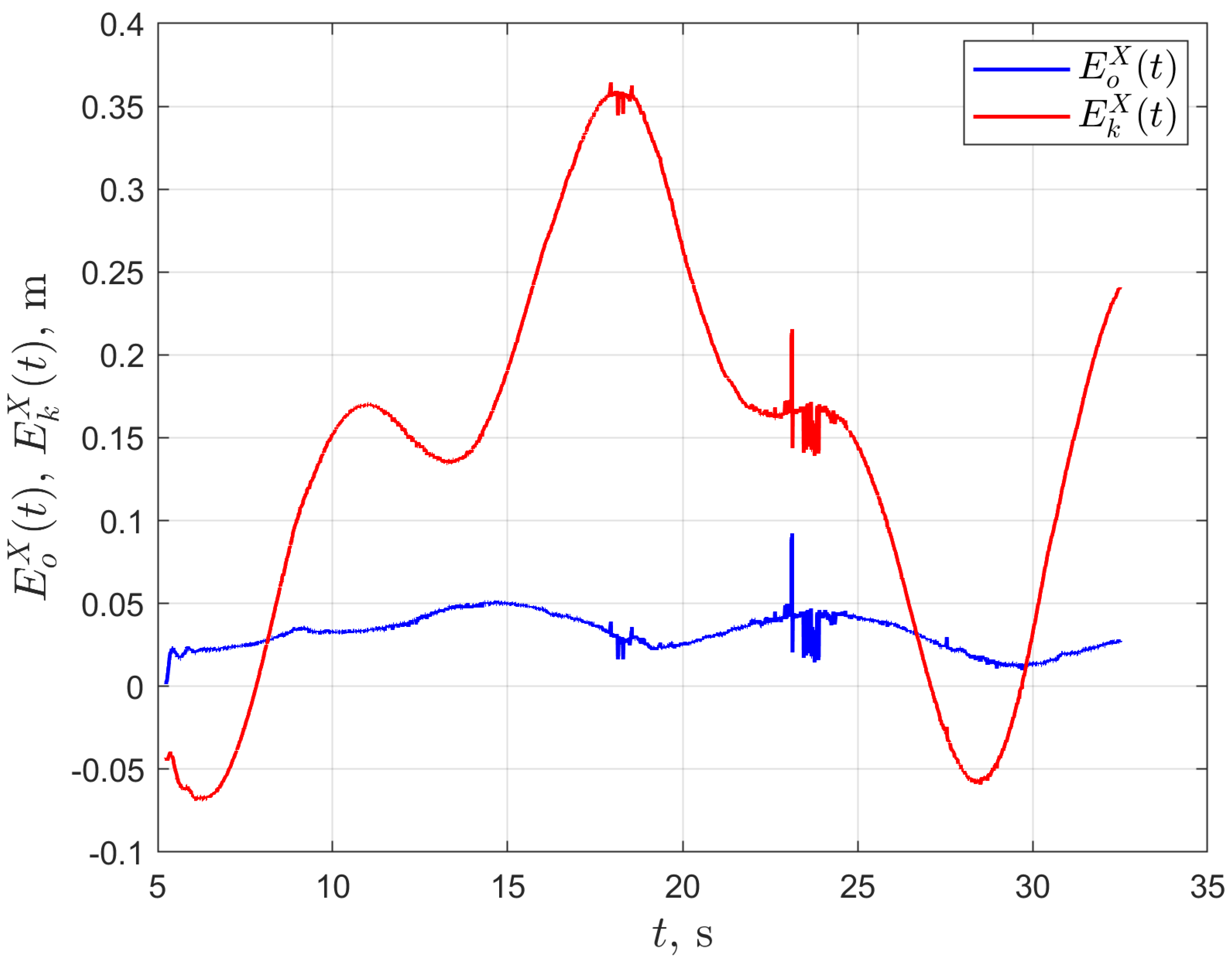
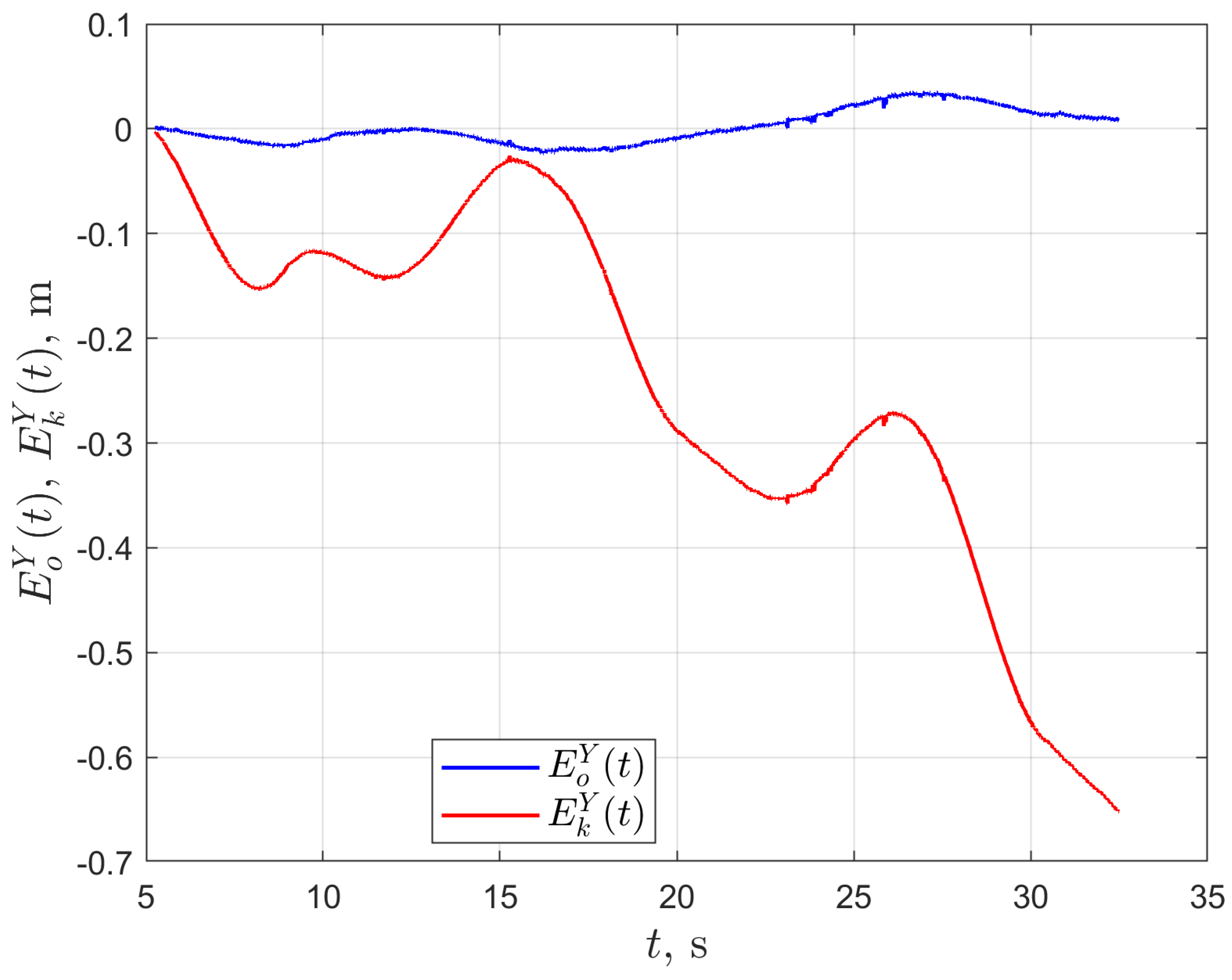
• Odometric localization errors for the x and y coordinates, defined as:

  $$E_o^X\left(t\right)=x_{opti}\left(t\right)-x_o\left(t\right),E_o^Y\left(t\right)=y_{opti}\left(t\right)-y_o\left(t\right),$$

  (9)

  where: $x_{opti}\left(t\right)$ (m)—the x coordinate of the position of the centre of the rigid body representing the robot at time t obtained from the OptiTRACK system, $y_{opti}\left(t\right)$ (m)—the y coordinate of the position of the centre of the rigid body representing the robot at time t obtained from the OptiTRACK system, $x_o\left(t\right)$—the coordinate x of the position of the centre of the rigid body representing the robot at time t obtained from odometric data, $y_o\left(t\right)$ the coordinate y of the position of the centre of the rigid body representing the robot at time t obtained from odometric data
• Localization errors based on the kinematics model forthe x and y coordinates, defined as:

  $$E_k^X\left(t\right)=x_{opti}\left(t\right)-x_k\left(t\right),E_k^Y\left(t\right)=y_{opti}\left(t\right)-y_k\left(t\right),$$

  (10)

  where: $x_k\left(t\right)$—the x coordinate of the position of the centre of the rigid body representing the robot at time t obtained from the model of kinematics, $y_k\left(t\right)$ the y coordinate of the position of the centre of the rigid body representing the robot at time t obtained from the model of kinematics.
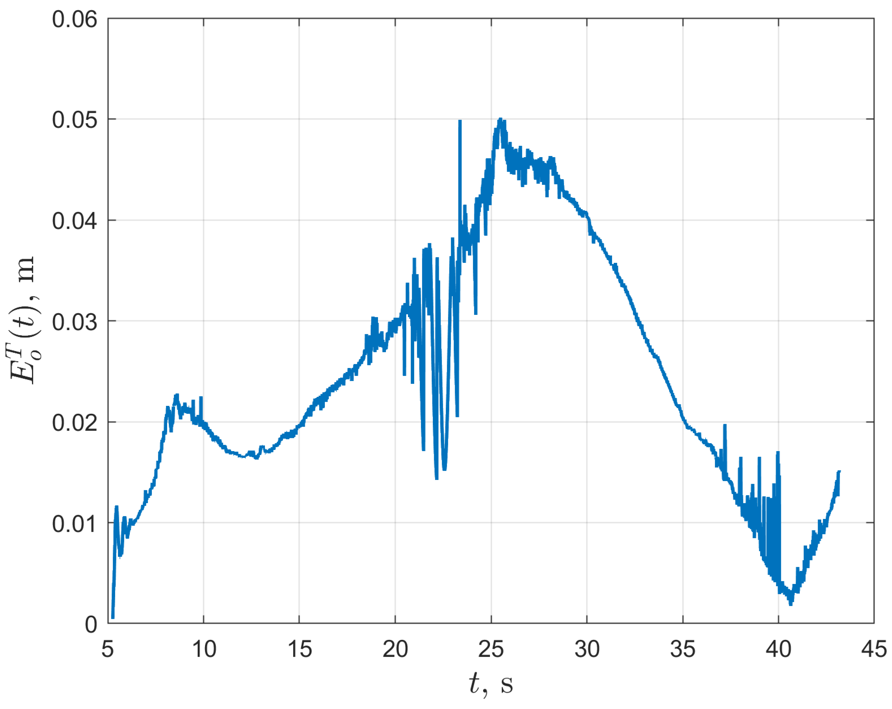
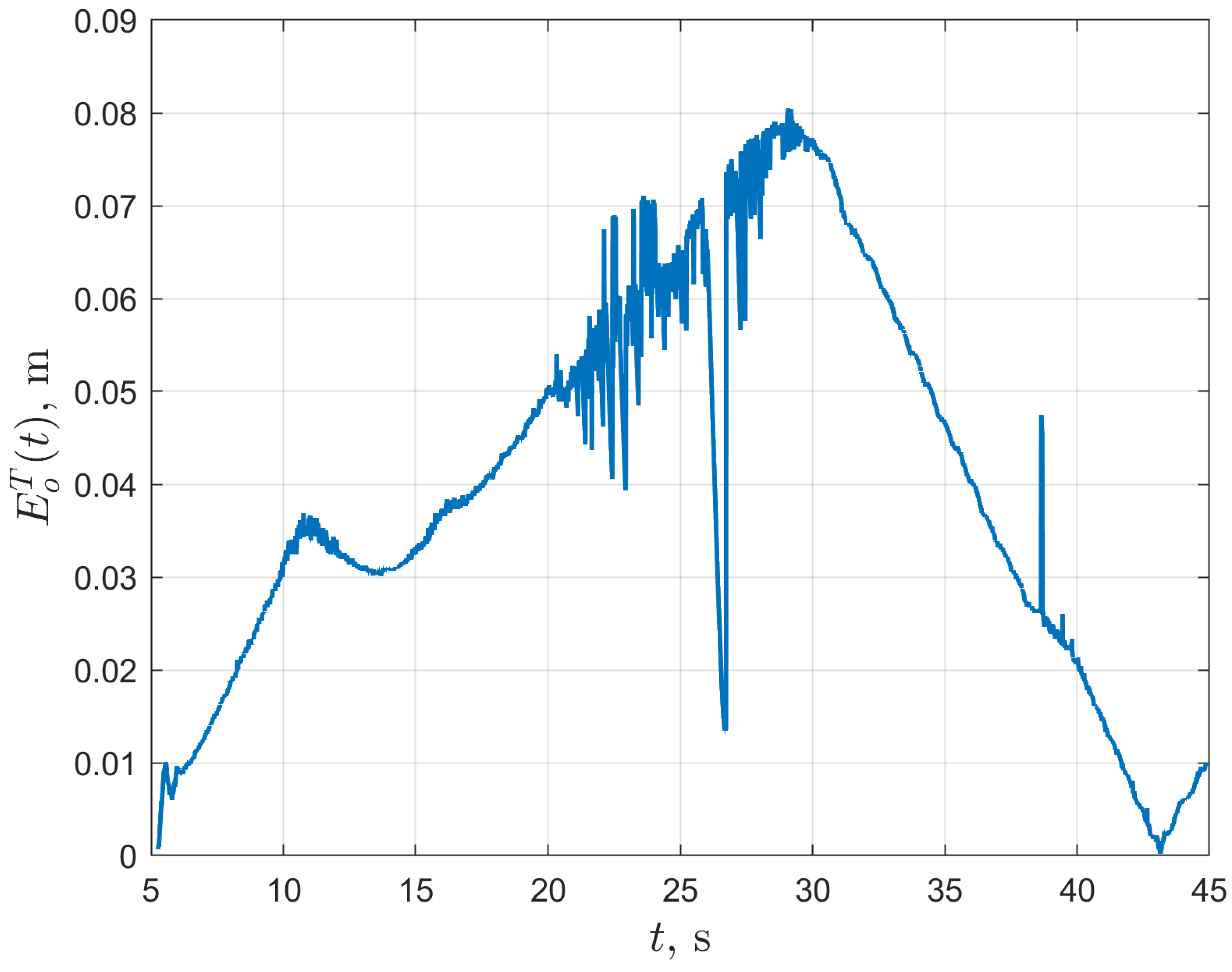
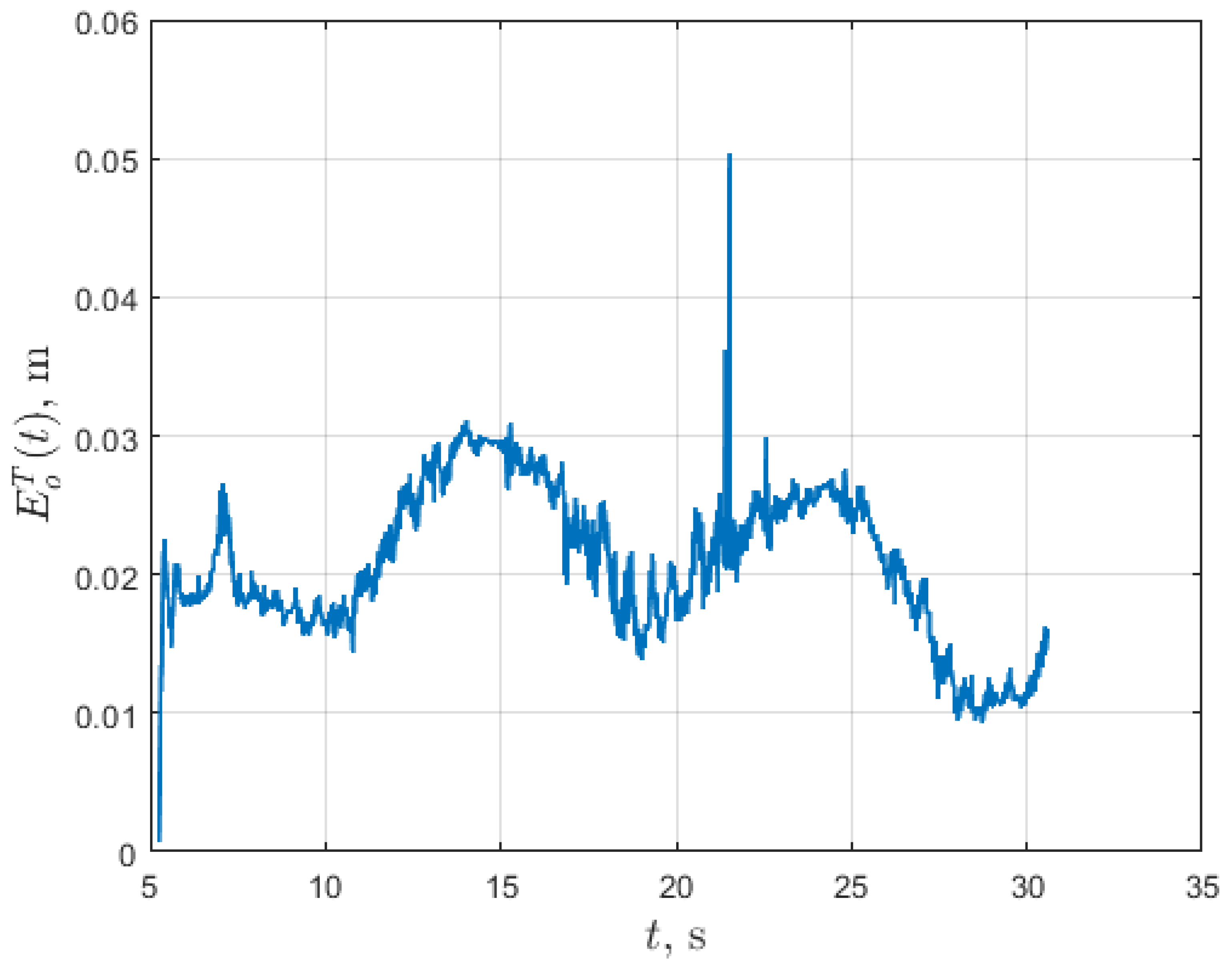
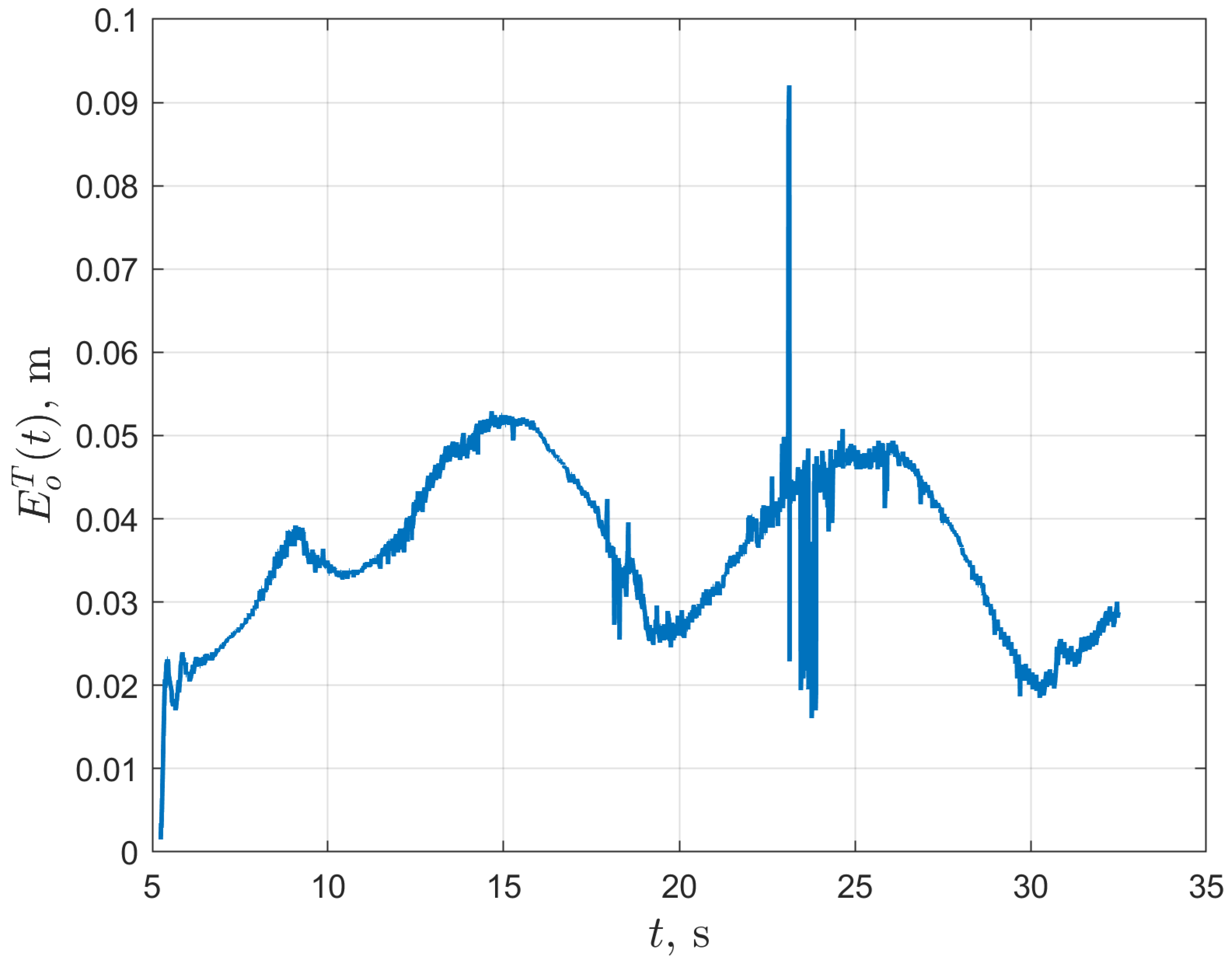
• The total odometric localization error described by the following equation:

  $$E_o^T\left(t\right)=\sqrt{{\left[E_o^X\left(t\right)\right]}^2+{\left[E_o^Y\left(t\right)\right]}^2}$$

  (11)
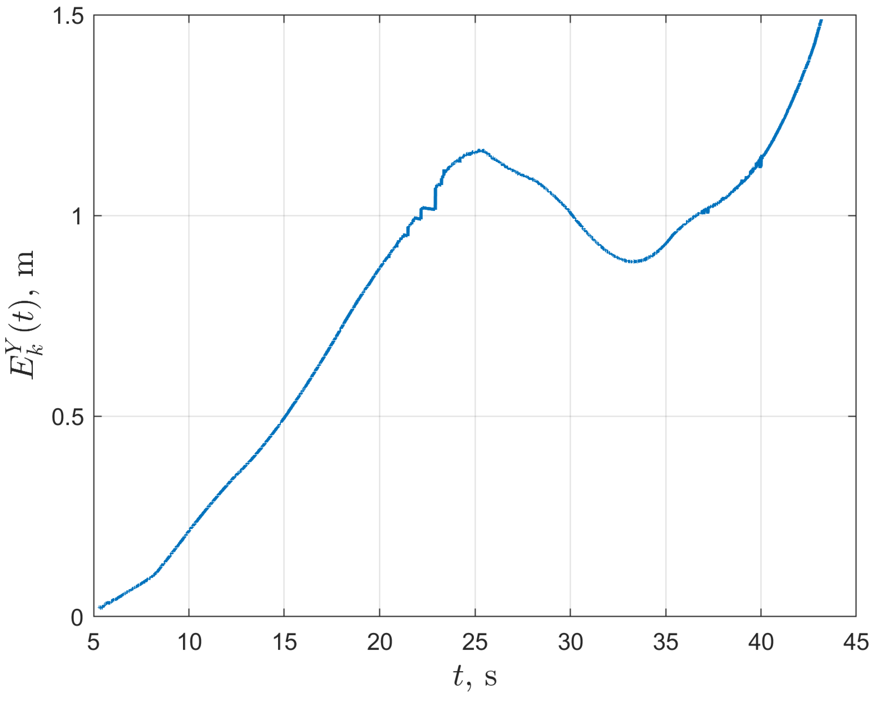
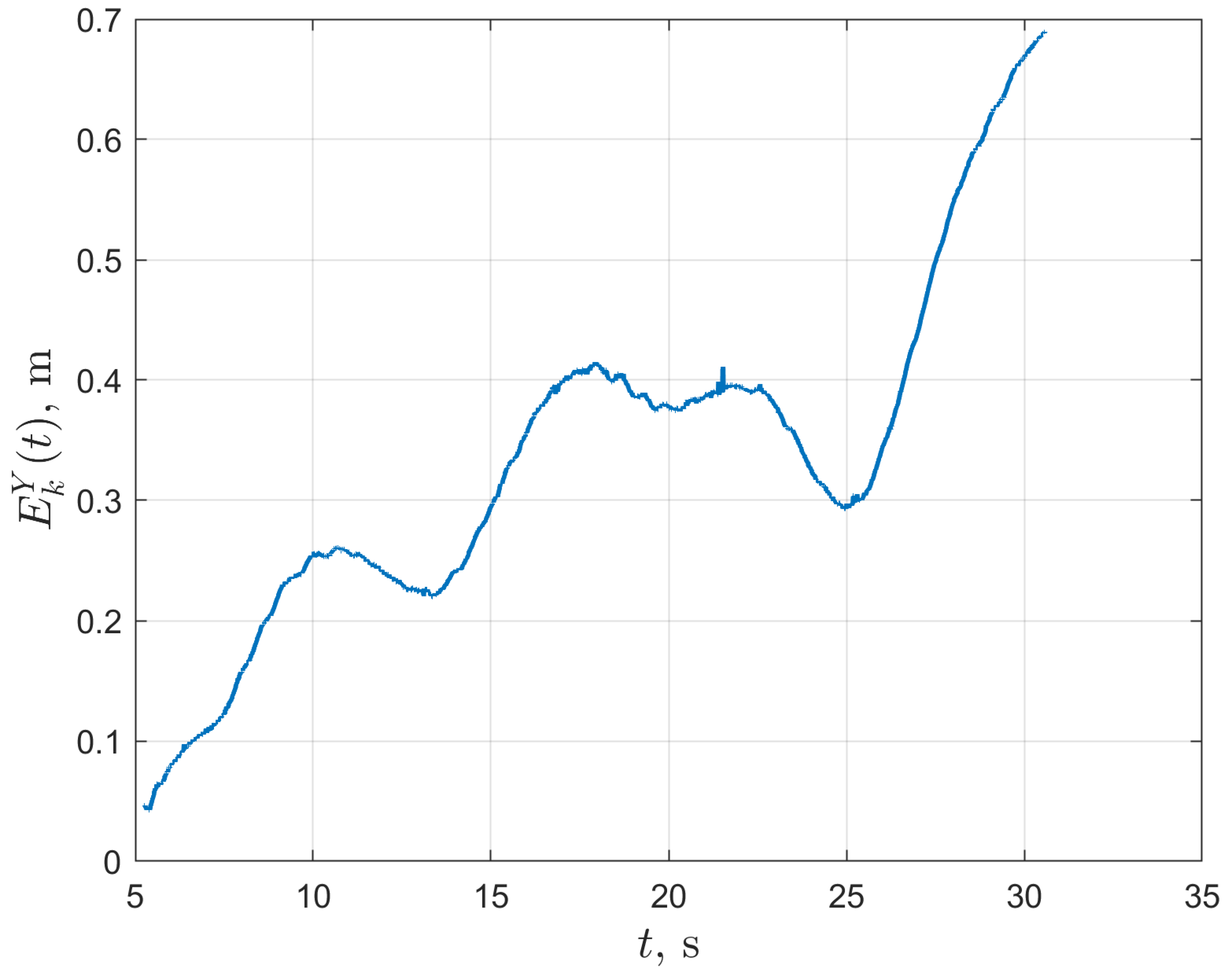
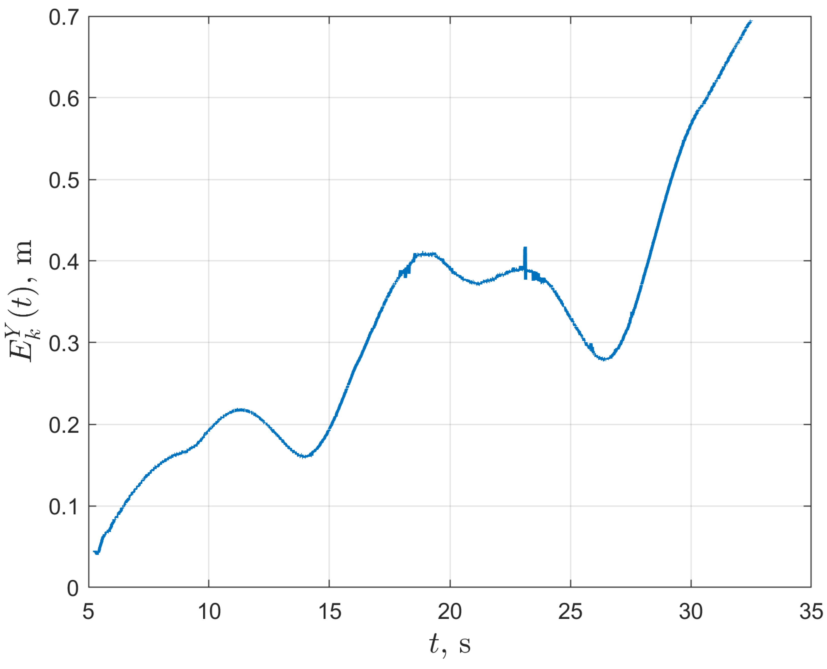
• Total location error based on the kinamatics model described by the following equation:

  $$E_k^T\left(t\right)=\sqrt{E_k^X{\left(t\right)}^2+E_k^Y{\left(t\right)}^2}$$

  (12)

The results of the analysis are presented later in the work.

3. Results

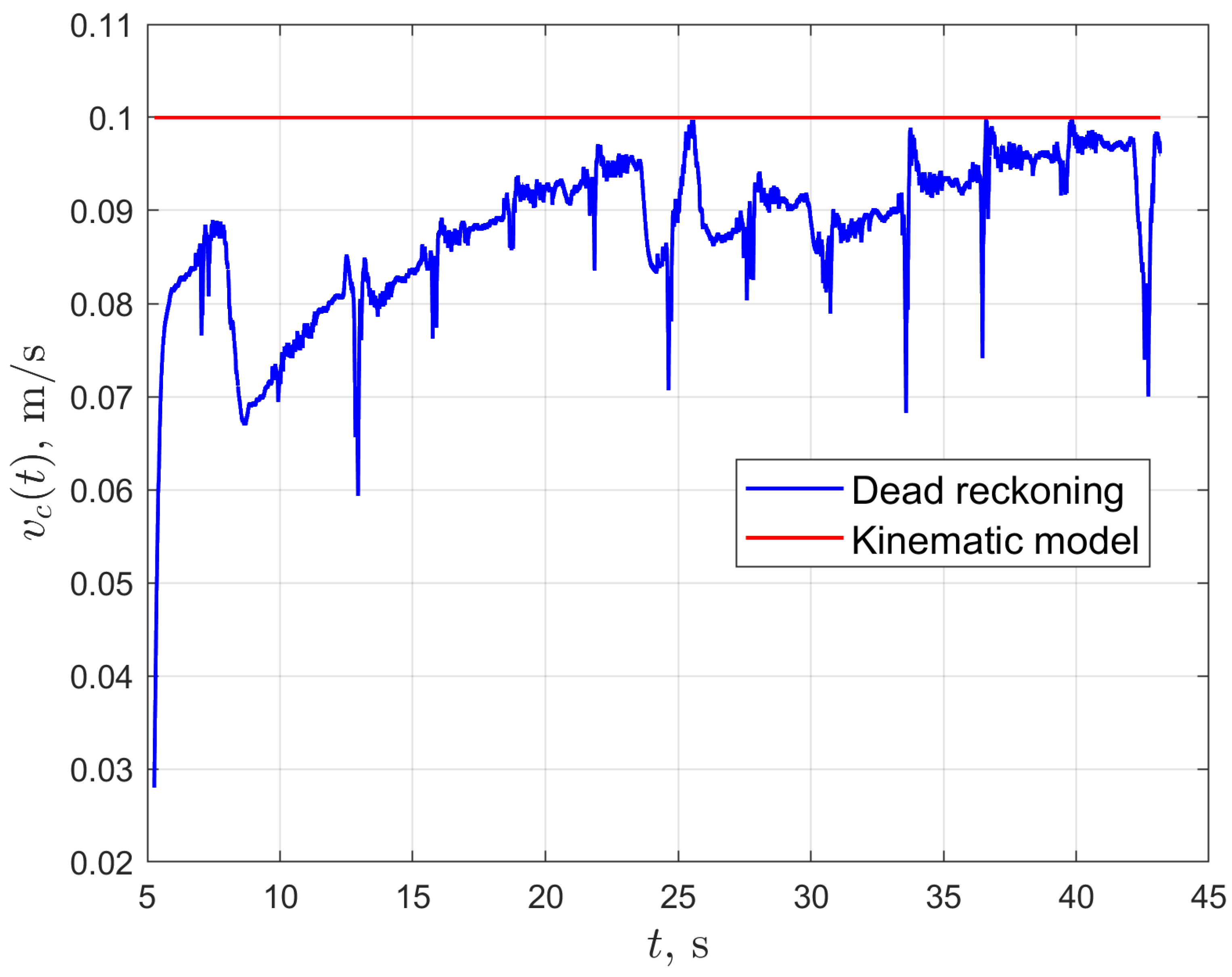
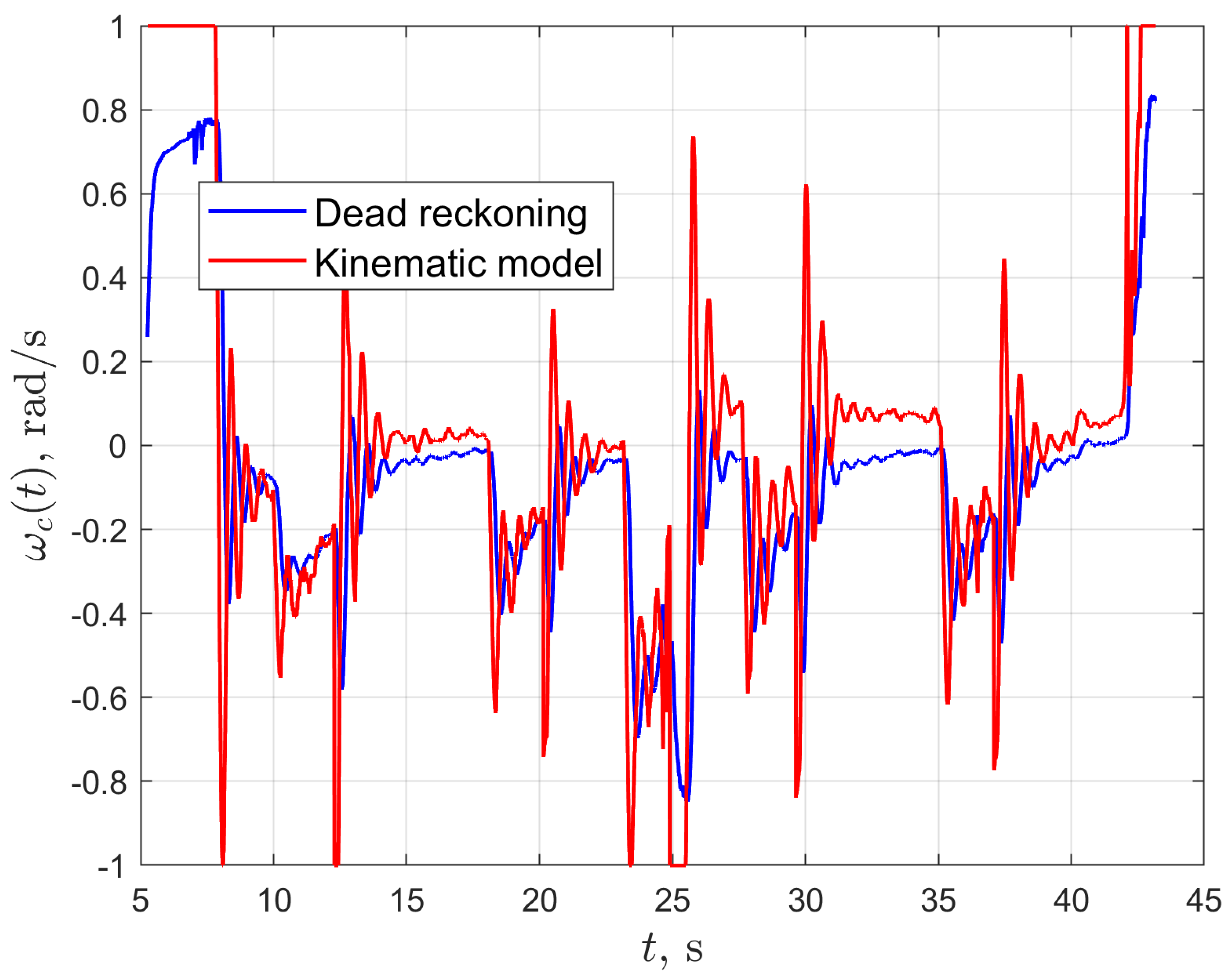
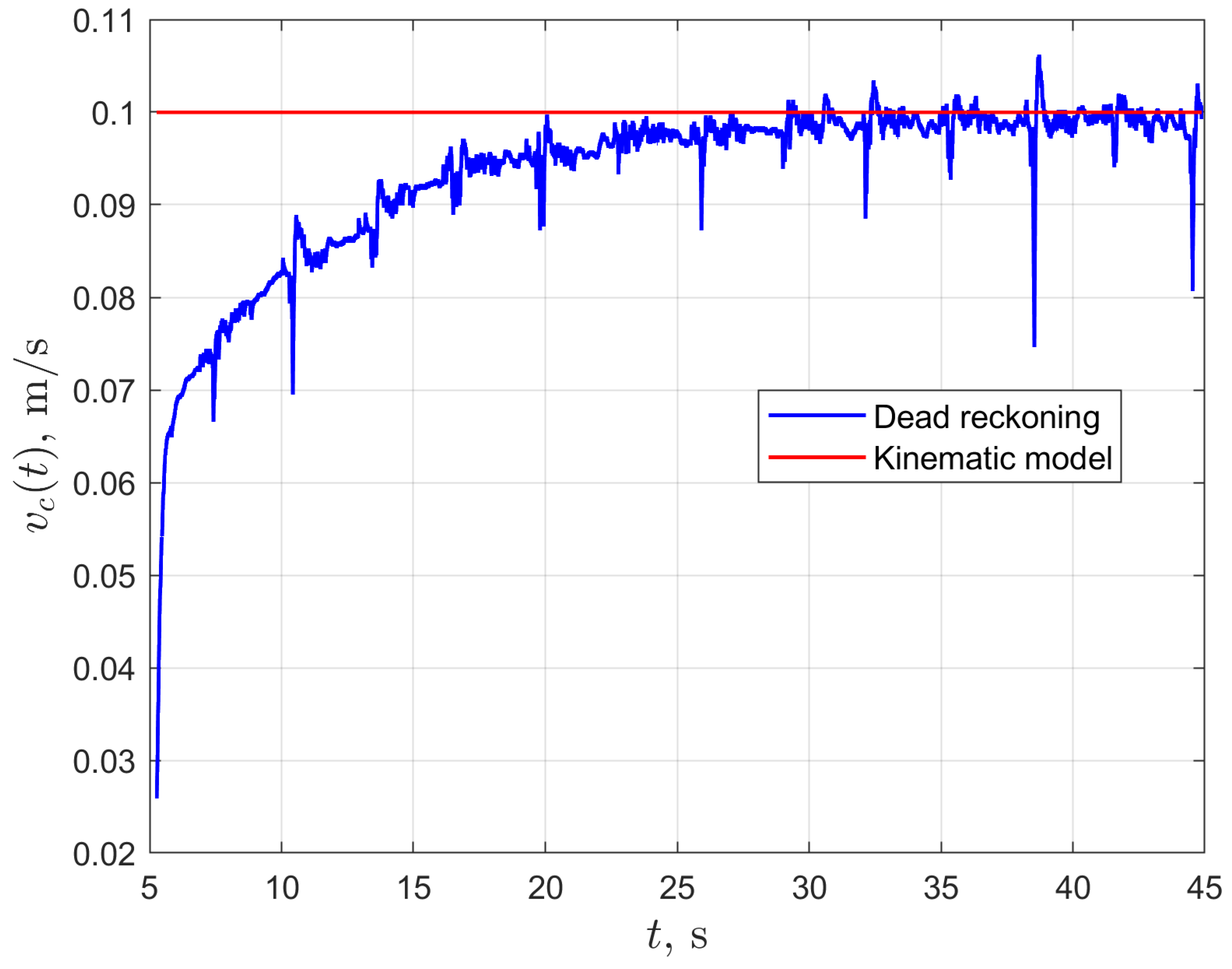
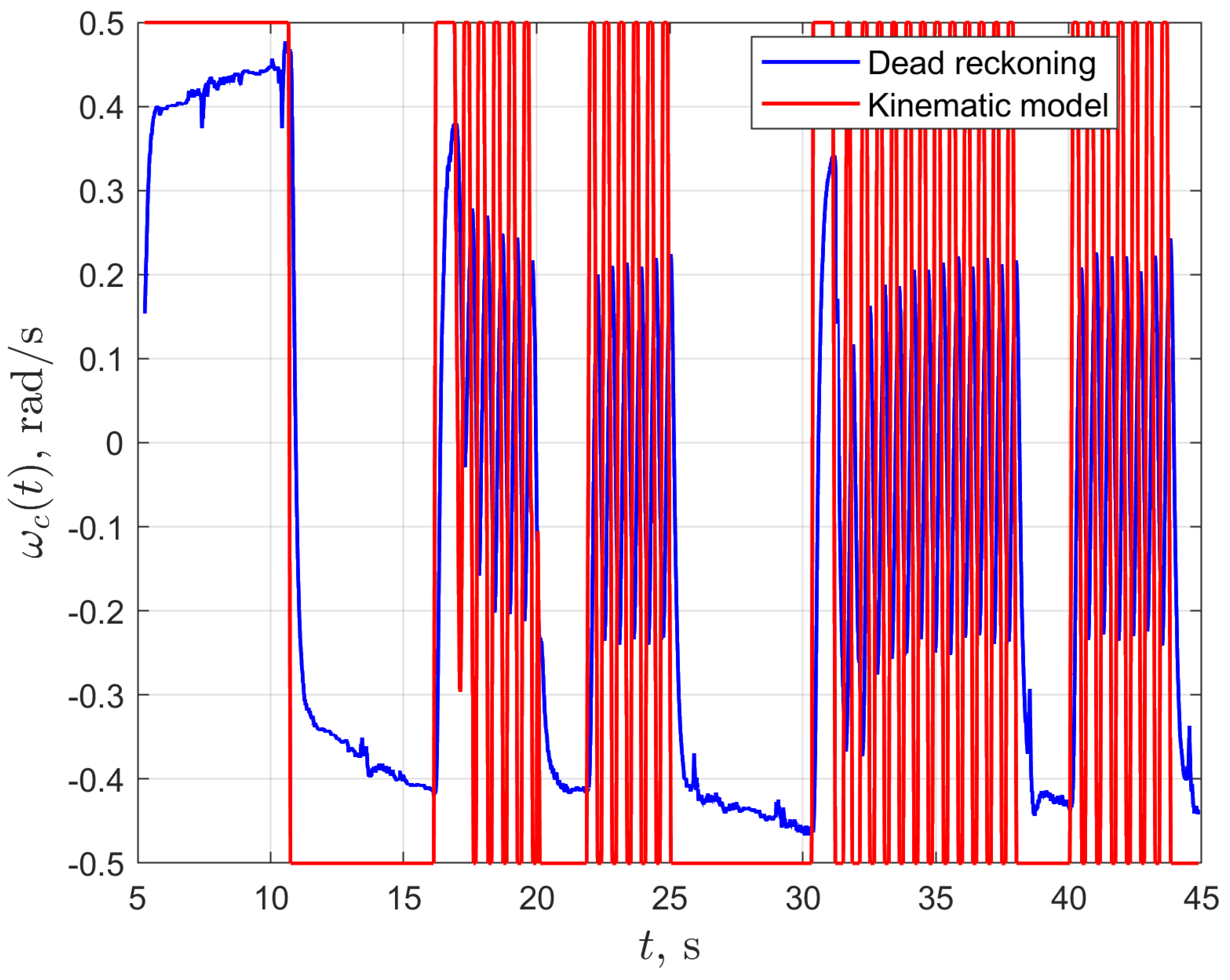
3.1. Results for $P_1$ Path

The selected results of tests carried out in accordance with the methodology described above are shown in Figure 11, Figure 12, Figure 13, Figure 14, Figure 15, Figure 16, Figure 17, Figure 18, Figure 19, Figure 20, Figure 21, Figure 22, Figure 23, Figure 24, Figure 25, Figure 26, Figure 27, Figure 28, Figure 29, Figure 30, Figure 31, Figure 32, Figure 33, Figure 34, Figure 35, Figure 36, Figure 37 and Figure 38. As mentioned above, the research has analyzed the accuracy of the location of the QBot 2e robot during the execution of two preset paths $P_1$ and $P_2$. The results of HIL simulation obtained during execution of path $P_1$ for simulation no. 1 (Table 1) are presented in Figure 11, Figure 12, Figure 13, Figure 14, Figure 15, Figure 16 and Figure 17. In Figure 11 the following are presented: the path set in the form of waypoints, the path captured by OptiTRACK system, the path determined on the basis of the model of kinematics (2) and (3) and the path determined on the basis of the odometric Equation (4).

The waveforms of linear and angular velocity of the robot determined on the basis of odometric data and model of kinematics are presented in Figure 12 and Figure 13.

In turn, in Figure 14, Figure 15, Figure 16 and Figure 17 were presented localization errors (9) and (10) determined for individual coordinates and the total location errors (11) and (12).

In Figure 18, Figure 19, Figure 20, Figure 21, Figure 22, Figure 23 and Figure 24 the results of HIL simulation number 4 (Table 1) obtained during the execution of path $P_1$ are presented. Similarly as in the case of simulation no. 1, in Figure 18 are presented the waypoints, the path recorded by OptiTRACK system and paths determined on the basis of the model of kinematics and Equation (4).

Figure 19 and Figure 20 show time evolutions of linear and angular velocity of the robot determined from odometric data and model of kinematics.

Time courses of location errors described by Equations (9) and (10) and time courses of total location errors (11) and (12) are shown in Figure 21, Figure 22, Figure 23 and Figure 24.

The values of Hausdorff distances $H_{OO}$ and $H_{OK}$ calculated when reproducing track $P_1$ in individual simulations are listed in

Table 3. The values of Hausdorff similarity measure calculated for $P_1$ path.

Simulation #	${\mathit{H}}_{\mathit{OO}}$ (m)	${\mathit{H}}_{\mathit{OK}}$ (m)
1	0.040	0.610
2	0.054	0.270
3	0.072	0.646
4	0.074	0.240

.

3.2. Results for $P_2$ Path

The results of HIL simulation carried out for path $P_2$ for simulation no. 1 (Table 2) are presented in Figure 25, Figure 26, Figure 27, Figure 28, Figure 29, Figure 30 and Figure 31. In Figure 25 are presented the following: the path set in the form of waypoints, the path captured by OptiTRACK system, the path determined on the basis of the model of kinematics (2) and (3) and the path determined on the basis of the odometric Equation (4).

The linear and angular velocity of the robot obtained on the basis of odometric data and model of kinematics are presented in Figure 26 and Figure 27.

In Figure 28 and Figure 29 the localization errors (9) and (10) calculated for individual coordinates were shown. In addition, the total localization errors (11) and (12) were presented in Figure 30 and Figure 31.

In Figure 32, Figure 33, Figure 34, Figure 35, Figure 36, Figure 37 and Figure 38 the results of HIL simulation number 4 (Table 2) obtained during the execution of path $P_2$ are presented. In Figure 32 the waypoints, the path recorded by OptiTRACK system and paths determined on the basis of the model of kinematics and Equation (4) were presented.

Figure 33 and Figure 34 show time evolutions of linear and angular velocity of the robot determined from odometric data and model of kinematics.

Time courses of location errors described by Equations (9) and (10) and time courses of total location errors (11) and (12) are shown in Figure 35, Figure 36, Figure 37 and Figure 38.

The values of Hausdorff distances $H_{OO}$ and $H_{OK}$ calculated when reproducing track $P_2$ in individual simulations are listed in

Table 4. The values of Hausdorff similarity measure calculated for $P_2$ path.

Simulation #	${\mathit{H}}_{\mathit{OO}}$ (m)	${\mathit{H}}_{\mathit{OK}}$ (m)
1	0.031	0.381
2	0.041	0.310
3	0.050	0.351
4	0.050	0.423

.

4. Discussion

Analyzing the results of research for the $P_1$ path and simulation #1, it can be stated that the location of the robot using the kinematics Equations (2) and (3) is burdened with a big error (Figure 11). The localization based on odometric data is much more accurate. The errors of the kinematics model result mainly from not taking into account the dynamic properties (i.e., inertia) of the robot. The influence of robot’s dynamics during execution of path $P_1$ can be observed in Figure 12 and Figure 13. The difference in accuracy can also be seen in Figure 13 and Figure 15. The maximum total localization error using dead reckoning shall not exceed 0.06 m and the maximum total localization error using kinematics equations shall not exceed 1.5 m (Figure 16 and Figure 17). Additionally, it can be observed that the error of localization using kinematics increases with time. Comparing Figure 11 and Figure 18 it was found that a smaller localization error with the model of kinematics is present in simulation #4. However, it should be stressed that also for simulation #4 the odometric localization is more accurate (see: Figure 18) In addition, in case of simulation #4 you can see a deterioration of tracking accuracy of the given path. This is mainly caused by the angular velocity limitation ${\omega }_{max}$. As before, Figure 19 and Figure 20 show the influence of dynamic properties. The error in localization of the model of kinematics is mainly due to the fact that it reacts in an inertial way, whereas in reality the robot has to accelerate. In Figure 20 the red line shows the effect of reducing the parameter $L_d$ (lookahead distance) of the pure pursuit controller. The graph shows large oscillations, which worsens the dynamic properties of the closed system and causes, among others, unnecessary energy losses. In Figure 21 and Figure 22 it can be seen that when angular velocity is limited (Table 1) to $0.5$ rad/s, the location error using the kinematics model decreases. Higher accuracy of localization using odometry is proved by values of Hausdorff measure collected in Table 3. It can be stated that the accuracy of odometric localization is several times higher than the accuracy of kinematic localization. Analyzing the results from Table 3 it was observed that the highest accuracy of odometric localization was obtained for simulation #1 and the lowest-for simulation #4. In turn, the highest accuracy of localization using the model of kinematics is observed for simulation #4 and the lowest for simulation #3.

Based on the results presented in Figure 25, Figure 26, Figure 27, Figure 28, Figure 29, Figure 30 and Figure 31 obtained for path $P_2$ (simulation #1) you can see that the odometric localization error is much smaller than the localization error based on the kinematics model. As in the case of path $P_1$ one of the reasons may be dynamic properties that are not included in the kinematics model described by Equations (2) and (3). The influence of robot dynamics is visible in Figure 26 and Figure 27. Analysing Figure 27 the research showed oscillations occurring during realization of path $P_1$ in simulation #1. This indicates too low value of the lookahead distance controller parameter. From the control point of view such a course of robot’s motion is very unfavourable. The difference in accuracy of the described localization methods can also be seen with reference to the components x and y shown in Figure 28 and Figure 29. In the study it was observed that the maximum total localization error calculated from odometric measurements $E_o^T\left(t\right)$ in simulation #1 does not exceed 0.05 m, while error $E_k^T\left(t\right)$ is almost $0.7$ m and increases with time. This means that as time passes, the localization of the robot obtained from the kinematics model differs more and more from the actual location. As with the #1 simulation, also for the #4 simulation, the accuracy of localization by means of the kinematics model is less than the accuracy of odometric localization (Figure 32). It is also visible that the limitation ${\omega }_{max}$ in the pure pursuit controller deteriorates the tracking accuracy of the desired path. In Figure 33 and Figure 34 the influence of robot dynamics for simulation is shown. The model of kinematics reacts at once, but in reality the robot has to accelerate. Additionally, Figure 34 shows the effect of increasing the lookahead distance parameter (red course) which led to a decrease in oscillation and improvement of dynamic properties. Similarly to simulation #1 a difference in accuracy of odometric and kinematic location was observed. This difference occurs both in relation to the coordinates x and y (Figure 35 and Figure 36) as well as total location errors (Figure 37 and Figure 38). Hausdorff distances presented in Table 4 allow stating that the accuracy of odometric localization is much higher than the accuracy of localization based on kinematics equations. The highest, in Hausdorff’s sense, accuracy of odometric localization was obtained in simulation #1, whereas in both simulations #3 and #4 comparable accuracy was obtained. In case of localization based on the model of kinematics, the highest accuracy was observed in simulation #2 and the lowest in simulation #4.

5. Conclusions

The paper describes the results of the robot localization carried out using two methods. In the first method the equations of forward and inverse kinematics were used to determine the location of the robot by means of formulas (2) and (3) on the basis of the position set by the pure pursuit controller. The second method carried out dead reckoning on the basis of measurements from encoders and gyroscope. To determine the accuracy, the OptiTRACK system was used, which recorded the actual path the robot was moving on. Two criteria were used to quantify the accuracy. The first–purely geometric—is a Hausdorff measure calculating the distance between two sets of points on the plane representing the path. The second measure is the time course of the Euclidean distance between individual points in which the robot was at the same time.

The studies compared the accuracy of odometric and kinematic localization for two paths given as an waypoint matrix. It was found that odometric localization allows following both set paths with satisfactory accuracy. Additionally, it was shown that the kinematics model for parameters from Table 1 and Table 2 is not able to provide the required accuracy and thus should not be used in control algorithms.

Finally, the results of the tests showed a high usefulness of the motion capture system and the Hausdorff measure to determine the accuracy of the QBot 2e robot location. The accuracy determination method described in this work can be used, among others, in prototyping new algorithms for controlling mobile wheeled robots. However, it should be stated that a great limitation of the proposed method of determining the accuracy of location is a need to install and calibrate a specialized set of cameras. For this reason, implementation of the method is only possible in laboratory conditions, in closed spaces.

References

- Le, A.; Clue, R.; Wang, J.; Ahn, I.S. Distributed Vision-Based Target Tracking Control Using Multiple Mobile Robots. In Proceedings of the 2018 IEEE International Conference on Electro/Information Technology (EIT), Rochester, MI, USA, 3–5 May 2018; pp. 142–149. [Google Scholar]
- Corke, P. Robotics, Vision and Control: Fundamental Algorithms in MATLAB, 2nd ed.; Springer Publishing Company Incorporated: Berlin/Heidelberg, Germany, 2017. [Google Scholar]
- Yamaguchi, H.; Nishijima, A.; Kawakami, A. Control of two manipulation points of a cooperative transportation system with two car-like vehicles following parametric curve paths. Robot. Auton. Syst. 2015, 63, 165–178. [Google Scholar] [CrossRef]
- Machado, T.; Malheiro, T.; Monteiro, S.; Erlhagen, W.; Bicho, E. Attractor dynamics approach to joint transportation by autonomous robots: theory, implementation and validation on the factory floor. Auton. Robot. 2019, 43, 589–610. [Google Scholar] [CrossRef]
- Niewola, A.; Podsędowski, L. PSD—Probabilistic algorithm for mobile robot 6D localization without natural and artificial landmarks based on 2.5D map and a new type of laser scanner in GPS-denied scenarios. Mechatronics 2020, 65, 102308. [Google Scholar] [CrossRef]
- Gharajeha, M.S.; Jondb, H.B. Hybrid Global Positioning System-Adaptive Neuro-Fuzzy Inference System based autonomous mobile robot navigation. Robot. Auton. Syst. 2020, 134, 103669. [Google Scholar] [CrossRef]
- Cook, G. Mobile Robots. Navigation, Control and Remote Sensing; John Wiley & Sons, Inc.: Hoboken, NJ, USA, 2011. [Google Scholar]
- Jadidi, M.G.; Miro, J.V.; Dissanayake, G. Gaussian processes autonomous mapping and exploration for range-sensing mobile robots. Auton Robot 2018, 42, 273–290. [Google Scholar]
- Fauser, T.; Bruder, S.; El-Osery, A. A Comparison of Inertial-Based Navigation Algorithms for a Low-Cost Indoor Mobile Robot. In Proceedings of the 12th International Conference on Computer Science & Education (ICCSE 2017), Houston, TX, USA, 22–25 August 2017. [Google Scholar]
- Kelly, A. Mobile Robotics, Mathematics, Models, and Methods; Cambridge University Press: Cambridge, UK, 2013. [Google Scholar]
- Dudek, G.; Jenkin, M. Computational Principles of Mobile Robotics; Cambridge University Press: Cambridge, UK, 2010. [Google Scholar]
- Bethencourt, J.V.M.; Ling, Q.; Fernández, A.V. Controller design and implementation for a differential drive wheeled mobile robot. In Proceedings of the Chinese Control and Decision Conference (CCDC), Mianyang, China, 23–25 May 2011; pp. 4038–4043. [Google Scholar]
- Rogne, R.H.; Bryne Torleiv, H.; Fossen Thor, I.; Johansen Tor, A. MEMS-based Inertial Navigation on Dynamically Positioned Ships: Dead Reckoning. IFAC-PapersOnLine 2016, 23, 139–146. [Google Scholar] [CrossRef]
- Sekiguchi, S.; Yorozu, A.; Kuno, K.; Okada, M.; Watanabe, Y.; Takahashi, M. Human-friendly control system design for two-wheeled service robot with optimal control approach. Robot. Auton. Syst. 2020, 131, 103562. [Google Scholar] [CrossRef]
- Ardentov, A.A.; Karavaev, Y.L.; Yefremov, K.S. Euler Elasticas for Optimal Control of the Motion of Mobile Wheeled Robots: the Problem of Experimental Realization. Regul. Chaotic Dyn. 2019, 24, 312–328. [Google Scholar] [CrossRef]
- Snider, J.M. Automatic Steering Methods for Autonomous Auto-Mobile Path Tracking; Technical Report, CMU-RI-TR-09-08; Robotics Institute, Carnegie Mellon University: Pittsburgh, PA, USA, 2009. [Google Scholar]
- Coulter, R. Implementation of the Pure Pursuit Path Tracking Algorithm; Carnegie Mellon University: Pittsburgh, PA, USA, 1990. [Google Scholar]
- Furtado, J.S.; Lai, G.; Lacheray, H.; Desuoza-Coelho, J. Comparative Analysis of OptiTrack Motion Capture Systems. In Advances in Motion Sensing and Control for Robotic Applications; Janabi-Sharifi, F., Melek, W., Eds.; Springer Nature Switzerland AG: Cham, Switzerland, 2018; pp. 15–31. [Google Scholar]
- Mashood, A.; Mohammed, M.; Abdulwahab, M.; Abdulwahab, S.; Noura, H. A hardware setup for formation flight of UAVs using motion tracking system. In Proceedings of the 10th International Symposium on Mechatronics and Its Applications (ISMA), Sharjah, UAE, 8–10 December 2015; pp. 1–6. [Google Scholar] [CrossRef]
- Magdy, N.; Sakr, M.A.; Mostafa, T.; El-Bahnasy, K. Review on trajectory similarity measures. In Proceedings of the 2015 IEEE Seventh International Conference on Intelligent Computing and Information Systems (ICICIS), Cairo, Egypt, 12–14 December 2015; pp. 613–619. [Google Scholar] [CrossRef]
- Little, J.J.; Gu, Z. Video retrieval by spatial and temporal structure of trajectories. In Proceedings of the Photonics West 2001—Electronic Imaging, International Society for Optics and Photonics, San Jose, CA, USA, 1 January 2001; pp. 545–552. [Google Scholar]
- Keogh, E.; Ratanamahatana, C.A. Exact indexing of dynamic time warping. Knowl. Inf. Syst. 2005, 3, 358–386. [Google Scholar] [CrossRef]
- Alt, H. The computational geometry of comparing shapes. In EffiCient Algorithms; Springer: Berlin/Heidelberg, Germany, 2009; pp. 235–248. [Google Scholar]
- Taha, A.A.; Hanbury, A. An Efficient Algorithm for Calculating the Exact Hausdorff Distance. IEEE Trans. Pattern Anal. Mach. Intell. 2015, 11, 2153–2163. [Google Scholar] [CrossRef] [PubMed]
- QUANSER. Available online: https://www.quanser.com/products/autonomous-vehicles-research-studio/ (accessed on 1 July 2020).
- OptiTrack. Available online: https://optitrack.com/ (accessed on 1 July 2020).