Abstract
This paper proposes an innovative approach to classify the losses related to photovoltaic (PV) systems, through the use of thermographic non-destructive tests (TNDTs) supported by artificial intelligence techniques. Low electricity production in PV systems can be caused by an efficiency decrease in PV modules due to abnormal operating conditions such as failures or malfunctions. The most common performance decreases are due to the presence of dirt on the surface of the module, the impact of which depends on many parameters and conditions, and can be identified through the use of the TNDTs. The proposed approach allows one to automatically classify the thermographic images from the convolutional neural network (CNN) of the system, achieving an accuracy of 98% in tests that last a couple of minutes. This approach, compared to approaches in literature, offers numerous advantages, including speed of execution, speed of diagnosis, reduced costs, reduction in electricity production losses.
1. Introduction
Photovoltaic (PV) systems are an environmentally friendly solution to achieve the objectives of sustainable development, production of green energy, and accessibility to energy resources promoted by Agenda 2030 [1]. PV systems represent a technology widespread in Italy and other countries, with over 800 sites in Italy [2], 30 GW of new power plants in China and a global total of installed power of 635 GWp recorded at the end of 2019 [3]. Over the time period of 2001–2013, many European countries have offered various incentives to promote new photovoltaic installations [4] according to the directives 2001/77/EC and 2009/28/EC [5]. However, these grants were unfortunately reduced between 2013 and the end of 2018 in Italy. In this scenario, it is essential to optimize plant performance and limit energy production losses to increase competitiveness on the market of electricity production from PV plants compared to fossil fuel technologies. The energy production of PV plants is affected by module or component failures (wiring, bypass diodes, etc.), malfunctions, or dust and soiling on the surface of the modules; the latter condition generally causes a decrease of 25% efficiency in comparison to the normal operating conditions [6]. For example, considering the PV system installed in Sicily (Italy) with a size of 50 kWp and consisting of 6 strings of 25 polycrystalline modules connected in series, according to the best working conditions, it can produce almost 70 MWh/year [7]. Considering instead that the system works normally with soiled modules due to dust deposits, debris and bird droppings, the energy production could be affected by 18 MWh/year, with a production loss of 26.7% [6].
To optimize the performance of a PV system, it is essential to use monitoring systems to quickly detect anomalies in normal operation [8] and investigate cleanliness of the modules by performing a periodic washing program. A commonly used monitoring method in recent years, due to its cost-effectiveness and rapid diagnosis, is the thermographic non-destructive test (TNDT), which is conducted by infrared thermography [9]. This technology allows different applications of pre-diagnosis and diagnosis of abnormal working conditions such as innovative electrical machines (Electromagnetic Aircraft Launch System—EMALS) [10], electric equipment [11] and in particular in the field of PV systems, because it allows us to identify the operating status of photovoltaic modules and other components (cables, junction boxes, etc.) without interrupting normal systems operation [12]. TNDTs can be used to identify any faults or malfunctioning conditions in the PV modules, i.e., all those conditions that cause local overheating. Deposits on the surface, such as dirt, dust and bird droppings, modifying the thermal exchange conditions between the module and the environment, cause local overheating. In general TNDT is performed by a skilled user (manually or using the support of drones, unmanned aerial vehicles [13] or autonomous underwater vehicles [14]), who must examine numerous thermographic images in a repetitive manner and with a high level of attention, since the manual calculation is subject to human error [15].
In order to develop a tool that automatically identifies abnormal operating conditions of PV modules [16,17,18,19,20], in this paper, the authors propose the application of the artificial intelligence technique. In particular, due to the use of a convolutional neural network (CNN), an automatic classification of thermographic images will be developed, distinguishing the effects of over-temperature on the surface of the photovoltaic module, caused by external factors (such as deposits on the surface of the modules), from those caused by faults. In this way, it is possible to distinguish thermographic images that show an anomaly condition due to a fault (cell breakage, delamination, etc.) from images that show the presence of dust, dirt and bird droppings on the module surface. To realize this application, open-source tools have been used, allowing this approach to be replicated freely by everyone.
This paper is subdivided as follows: Section 2 addresses energy production in a PV system and its influencing parameters; Section 3 explores the effects of soiling on the PV system; Section 4 proposes TNDT as a diagnostic method of PV abnormal operating conditions; Section 5 and Section 6 propose a CNN for the automatic classification of thermographic images; Section 7 displays the results; Section 8 provides the conclusions.
2. PV Systems Efficiency
The annual electricity produced by a photovoltaic system is related to the performance of the entire PV system and is affected by all factors which, under normal operating conditions, cause its variation, such as [21]:
- (1)
- Plant characteristics: tilt angle, orientation, type of module coverage, module connections, etc.;
- (2)
- Environmental conditions: temperature, humidity and wind speed;
- (3)
- Site characteristics: local vegetation, traffic, air pollution, proximity to the sea.
In the literature, the annual electric energy production is estimated using Equation (1), which shows the relationship with previous conditions [22]:
where
- is the annual electrical energy supplied to the network (kWh/year);
- is the peak power at standard test conditions (STC) (kWp);
- is the solar irradiance at STC (W/m2);
- is the total annual solar irradiation on the PV module plan (kWh/(m2∙year));
- is the Azimuth angle of the modules;
- is the tilt angle of the modules;
- is the performance ratio;
- is the estimated loss factor due to shadowing;
- is the additional loss factor; this parameter includes the presence of different factors, such as shading, mismatching, dust, soiling and possible module failures.
(STC: temperature of 25 °C, irradiance of 1000 W/m2 and air mass 1.5 (AM1.5) spectrum).
The depends not only on the environmental and installation conditions of the PV system but also on failures and losses due to shading [23], dust and degradation [22,24,25] as shown by the coefficients and which consider the efficiency reduction when these phenomena occur. These phenomena affect the functioning of the module in differing invasive ways: failures can be catastrophic, locking the single-cell or module operation, or by deterioration, reducing the operation of the single cell or the entire module progressing in the file of the systems. The losses affecting PV systems can be of several types and each of them can affect the operation of the PV module in a more or less invasive way [12].
3. Dust, Soiling and Debris
In PV systems, the efficiency of the module is reduced by 10–25% due to the presence of soiling, dust and debris deposited on its surface [21]. These phenomena determine a limitation of the incident solar radiation on the cell surface, which will operate at lower performance than the adjacent cells; since the cells are interconnected, there is a reduction in the performance of the other cell due to the mismatch effect [26]. Dust deposits are a complex phenomenon and are influenced by the different environmental and climatic conditions of the site [27]. The dust is generally composed of small solid particles, of 500 micrometers in diameter, dispersed into the atmosphere from different sources, such as dust raised by the wind, pedestrian and vehicular movement, volcanic eruptions and pollution [21]. For example, a module installed in an area subject to sand loads from desert winds will be exposed to higher dust deposits than a module subject to winds from other climate zones [21]. According to studies by Goossens et al. [28], the dust deposit decreases with increasing wind speed and is influenced by the orientation and tilt angle of the module. In fact, modules with higher inclination angles will be subject to minor dust accumulation due to gravity. The performance of a PV system is also influenced by the environment surrounding the installation site: under the same installation and operation conditions, 6.9% of losses occur if the PV system is built on sandy soil, and 1.1% of losses if it is built on compact ground [29], this generates a loss of according to the parameter indicated in Equation (1).
The density of the dust layer deposited on the module decreases its efficiency due to the reduction of solar radiation absorbed by the module, as demonstrated by EL-Shobokshy [30]; in fact, dust attenuate the irradiance in a spectrum-dependent manner. This occurs because the deposit of dust causes a variation of the transmittance in the glass of the photovoltaic cell, varying the dependence of angle of incidence of the solar radiation on the PV cell surface, producing a significant degradation of the solar conversion efficiency [31,32]. Montes et al. [33] demonstrate the impact of the Sahara Desert dust on the performance of a PV system installed in the Canary Islands, in which wind storms carry a thin reddish-brown layer. The dust deposits on PV module surfaces cause a reduction of between 5% and 7% due to a solar radiation reduction between 2% and 3% [33]. The loss of efficiency of the PV module also depends on the period in which the dust is present on the cell surfaces; according to a study conducted by the University of Màlaga in Spain, it is generally possible to have a daily loss of more than 20% [34]. According to the study of Hassan et al. [35], for a period of 1 to 6 months of exposure of PV modules to airborne dust, there is a rapid reduction in efficiency during the first 30 days of dust exposure, which gradually continues over time.
4. Thermographic Analysis to Detect the States of PV Modules
The TNDT is commonly used as a diagnostic method for predictive maintenance to monitor existing conditions, as it provides quick, cost-effective and efficient inspection of large or difficult-to-access PV systems without interrupting normal system operation [12].
The TNDT can be used to analyze PV systems of different sizes, layouts and characteristics; the rapidity of this analysis depends on the image acquisition methodology and the size of the PV system. The TNDT can be performed traditionally by a qualified ground-based operator or by Remotely Piloted Aircrafts (RPAs) such as drones [36]. RPA was identified as a cost-effective approach that allows reducing the conventional inspection time of PV systems by 10–15 times [37]. As reported in various studies [36,38], a 1 MW size plant can be inspected with TNDTs supported by RPA in about 5–8 min; this provides a considerable advantage compared to the execution by a qualified ground-based operator, because the TNDT can be performed only for 4 or 6 h during the day [37], according to the standards provided by IEC TS 62446-3: 2017 [39].
The costs for the execution of the TNDT depend on the size of the PV system and on the time required to perform the tests; in fact, the price of RPA is EUR 2000 for standard equipment and EUR 28,000 for high-performance and customized systems [40]. According to the study of Grimaccia et al. [41], the use of RPA for the inspection of a 1 MW PV plant is about 6–10% of the annual maintenance costs, corresponding to USD 50 per kW. Comparable studies conducted by Quarter et al. [42] have shown a cost increase of less than 5% of the average annual maintenance cost for TNDT applications in PV plants with a size of from 0.2 to 1 MW.
The TNDT method is based on the detection of infrared radiation emitted by objects in proportion to their temperature, according to Planck’s law. The distribution of the surface temperature of the body allows one to determine any anomalies in its operation. The most common malfunction or failure in a PV module is highlighted by an increase in the surface temperature, which can be detectable in thermographic images. Some examples of failure cases are [43] the manufacturing defect, the damage, the bypass diode defect, and faulty interconnection of modules appearing in the thermal image as overheating [44]. However, shadow, dust, and bird droppings also appear in thermographic images as local overheating [45]. Local overheating associated with a fault condition shows a temperature increase in the order of tens of degrees compared to normal operating conditions [15]. This generally has a well-defined geometric and distinguishable shape for the different types of faults [9]. Figure 1 shows a thermographic image acquired on the glass side of the module, displaying the presence of a hot spot due to a failure on the PV cell.
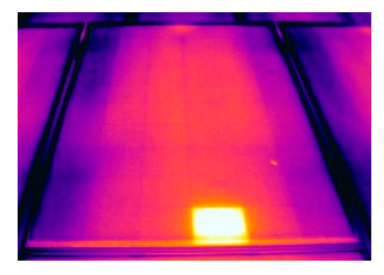
Figure 1.
Thermographic image of a hot spot on the photovoltaic (PV) cell.
On the contrary, dust and soiling phenomena cause localized overheating of some degree, widespread in the area of the dirt cover, causing a visual effect that depends on the different types of dirt [45]. For example, as shown in Figure 2, dirt on the module surfaces can be considered as a semi-homogeneous deposit or hot strips (if the dirty module has been exposed to light rain).
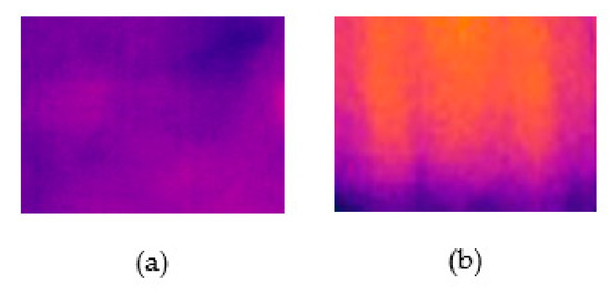
Figure 2.
Thermographic image of a PV module: (a) dirty; (b) dirty after light rain.
Bird droppings, instead, are detected as a local overheating of irregular geometric shape, whose temperature increase is a few degrees higher than the normal operation of the module in the environmental conditions of the site. The increase in temperature generally occurs in the range of 1 to 3 degrees Celsius [46], but as indicated in [12] the temperature can increase by 5 degrees Celsius. An example of a local overheating caused by bird dropping is shown in Figure 3.
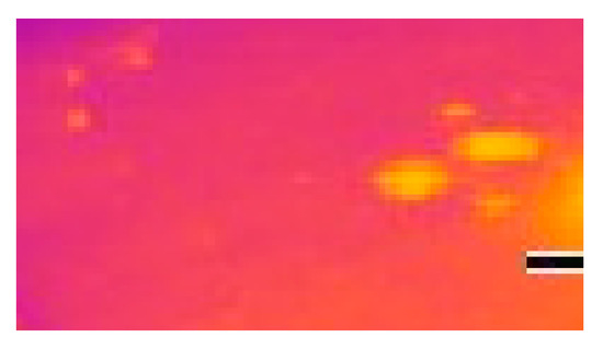
Figure 3.
Thermographic image of a PV module with bird droppings.
5. Convolutional Neural Network to Classify Thermographic Images
The thermographic images allow one to detect anomalous operating conditions, especially in medium- and large-size systems; the control of the thermographic images, as well as their acquisition, must be carried out by an expert operator who is able to distinguish between different operating conditions of the system. This is a time-consuming operation that can be reduced by automating the image classification process supported by artificial intelligence techniques. In this paper, an artificial neural network has been developed, trained and used for the classification of thermographic images. The artificial neural network is a network or circuit of neurons, composed of artificial neurons or nodes that, through mathematical functions, simulate the information transmission of information as between biological neurons [47]. Artificial neural networks allow the solving of complex problems in different domains, such as classification analysis of big data. Classification can be interpreted as the ability to identify a specific subject that corresponds to a specific category [48]. For a human being, this skill is learned in childhood, due to the presence of a teacher (parent) who helps the child to associate the name of an object with the object itself; similarly, artificial intelligence supported by an artificial neural network can learn to identify the category of an object in the form of probability of affiliation due to the recognition of unique patterns [49].
The CNN is a feed-forward network made up of several layers of connected neurons. The layer in the neural network that receives the input is based on the convolution function, hence the name of the CNN. The functioning of the CNN allows numerous applications for image classification, as it is inspired by the organization of the animal visual cortex [50]. The CNN model is generally formed by a succession of layers ruled by different mathematical functions to extract the patterns of image recognition and then classify them [50]; the images are input into the CNN as an array of pixels, the value of which is indicative of the light intensity of the point. A CNN example is shown in Figure 4.
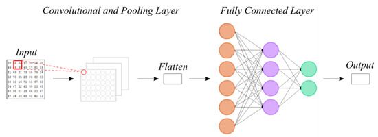
Figure 4.
Structure of the convolutional neural network (CNN).
The convolutional layers identify the input characteristics through the application of the convolutional function in the discrete domain. The convolution of the input matrix is realized using a convolutional matrix, called a kernel, applied with a specific application step [51]. The convolutional function is replicated for the entire section of the input matrix and returns a matrix, called an activation map, which contains the representative characteristics of the input [48]. An example of convolution function using a (3, 3) kernel applied in input matrix is shown in Figure 5.
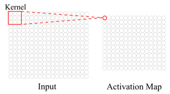
Figure 5.
Graphic example of convolution function.
Convolutional layers are alternated with pooling layers, which sample the activation map by reducing its spatial dimensions. In the pooling layers, the matrixes are sampled using a mathematical function, such as Max-pooling or Avg-pooling, which select the pixels with a maximum or average value to highlight specific characteristics of the image [52]; an example of Max-pooling and of Avg-pooling functions is shown in Figure 6.
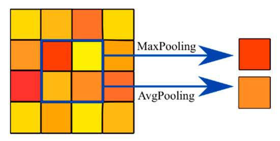
Figure 6.
Graphic example of Max-pooling and Avg-pooling functions.
Fully connected layers contain perceptrons that, due to learning, distinguish the characteristics of the inputs and identify the associated class [53]. These layers receive the activation map as a vector due to the flatten function. The flatten function converts the dimension of the activation matrix into a one-dimensional array, and this allows fully connected layers to receive input data; an example of an unrolling arrays is shown in Figure 7.
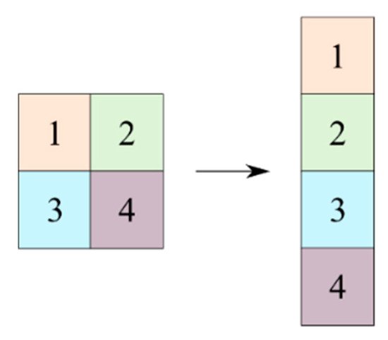
Figure 7.
Graphic example of the flatten function.
In fully connected layers, the perceptrons are activated in a specific percentage by the activation function , which depends on an array (Z) containing the number of neurons of the previous layer and the current layer, the input vector (X) and bias vector (b) [54], as shown in Figure 8.
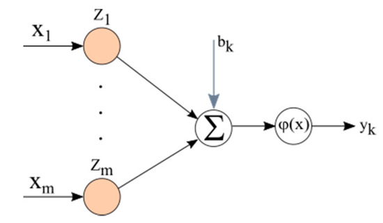
Figure 8.
Graphic example of fully connected layers function.
A common activation function is the rectified linear unit (ReLU), which activates the perceptrons if the input vector is greater than zero [55], as shown in Equation (2).
The CNN is configured by evaluating several parameters, such as the choice of the optimizer for perceptrons training, the number of epochs and the batch size [52]. The optimizer is used in fully connected layers to compile and train the CNN model, enabling the modification of the benchmark value (weights) used to train the CNN perceptrons for the recognition of the two categories, improving the convergence speed to a solution (category) and increasing its accuracy. The most used optimizers are Adam and stochastic gradient descent (SGD). The batch size is the number of samples sent simultaneously to CNN layers, while the number of epochs is the number of CNN learning cycles [56]. The CNN parameters are chosen to limit the overfitting problem, which occurs when the algorithm learning is adapted to the samples of the training phase, failing to recognize its characteristics. Consequently, there is a significant increase in error due to the non-sent classification of the inputs sent during the test phase [57].
6. Dust and Hotspot Classification Using Convolutional Neural Network
In this study, a CNN was implemented, which is capable of classifying the thermographic images based on the thermal anomalies on the surfaces of the PV modules. The classification was based on the geometric characteristics of local overheating, allowing the CNN to classify thermographic images acquired with different color scales and to distinguish them in the “dust” and “fault” categories. The CNN was developed based on open-source software and tools; in particular, Python programming language and the TensorFlow and Keras libraries were used. The CNN allows the automatic acquisition of training and test images, which are pre-processed through different techniques, and returns as output the probability that the image belongs to a category. CNN operation is shown in Figure 9. In detail, CNN receives as input a set of images collected in a dataset, which are automatically pre-processed to highlight their main recognition characteristics. Subsequently, the images are sent to the CNN’s learning algorithms that vary in terms of parameters and characteristics, according to the quality of the results achieved. A supervised learning classification is performed by assigning a category label to the training images.
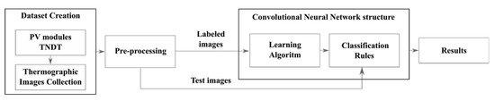
Figure 9.
CNN construction.
6.1. Dataset Creation
To generalize the application, various thermographic images of different PV Italian power plants were considered; these images were acquired in several legacy PV systems of different characteristics throughout the Italian territory, using different thermal camera technologies, resolution and settings (color scales). The image dataset used is composed of 600 sections, of which 240 images were used for the training dataset for each of the categories, while 60 images were used for the test dataset for each of the categories. The training and testing dataset were created by dissecting relevant parts of the thermographic images to highlight the geometric shapes of the hot spots for the cases of interest. The sectioning of the thermographic images was performed in order to limit the coexistence of the two categories in the same image, reducing the presence of noise.
6.2. Pre-Processing Phase
To reduce noise and increase the neural network performance in terms of precision, accuracy and speed of execution, different types of pre-processing were applied to the false color images (C) obtained from the thermographic analysis. All images individually acquired by the operator or extracted as frames from videos were subjected to a normalization phase of the light intensity value of pixels and homogenization of the number of pixels. The normalization was performed by showing the pixel light intensity value on the 1/255 scale. The homogenization of images, on the other hand, was achieved by sending a defined number of pixels of the image to the neural network, according to the proportions between its dimensions (width and length). Other techniques for varying the light intensity of the pixels carried out to highlight the geometric shape of the local overheating shown in the image and in Figure 10 are as follows:
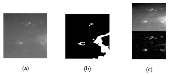
Figure 10.
Pre-processing images: (a) grayscaling; (b) thresholding; (c) box blur and Sobel–Feldman filters.
- -
- Grayscaling (G): The color of the thermographic images is generally represented in a different “false color” scale or grayscale depending on the setting and type of thermal image camera.
- -
- Thresholding: To highlight the discontinuities of the modules surfaces, a black and white threshold (or binarization) of the light intensity value of the pixels was performed. In addition, dilated and erodible filters were used to increase the image quality and reduce noise (e.g., salt and pepper noise). The dilator filter allows one to determine the maximum local value of the light intensity of the pixels, expanding the area of the pixels with the highest light intensity value. The erode filter, on the contrary, allows one to identify the minimum local value, expanding the area of the pixels with the lower light intensity value [58].
- -
- Box blur and Sobel–Feldman filters (F): A combination of two images was used to compare the application of the box blur and Sobel–Feldman filter. The box blur filter was used to blur the thermographic image to reduce discontinuities shown on the surfaces of the module [59]. On the contrary, the Sobel–Feldman filter was used to highlight the edges and discontinuity [60].
Another pre-processing phase consists of using the augmentation techniques of the images. These techniques allow one to increase the number of images present in the dataset due to the roto-translation and zooming of pixels [61] to train the CNN to also recognize thermographic images in which the local overheating characteristics are not perfectly identifiable, as is the case of the use of drones. In addition, technical augmentations allow a reduced image number for CNN training, permitting the application to be used with a limited amount of available data. Examples of augmented images are shown in Figure 11. The use of augmentation allows a reduction of the overfitting problem; due to this technique, it is possible to send as input several samples of the same image to the CNN, highlighting different pixel area [62].
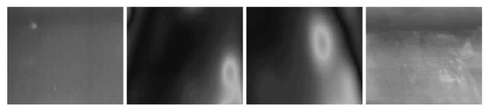
Figure 11.
Augmentation techniques.
6.3. CNN Models and Configurations
The CNN was developed with different models and configurations to identify the highest thermographic imaging classification performance and to increase convergence. The CNN structure was created using the functions and configurations shown in the flow chart in Figure 12; the number of layers was chosen according to the proposed models.
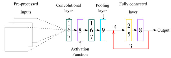
Figure 12.
Flow chart of the proposed CNN.
The following configurations were used:
- Image size: The size of 3500 pixels was selected.
- Number of perceptrons: 20% of the image size was selected as the number of perceptrons.
- Number of epochs: The number of epochs of 15, 30, 45 was chosen to reduce overfitting problem, considering that the images used do not contain faults and dirty parts in the same frame; this helps CNN learn samples faster.
- Batch size: The batch was selected in a small size of 5 and 10 to avoid the overfitting problem and to improve the accuracy of the CNN.
- Optimizer type: Adam and Stochastic Gradient Descent (SGD) optimizers, both with a learning rate of 0.01, were compared to evaluate the quality and speed of convergence.
- Number of filters: The choice of the number of filters was made in accordance with the operation of convolutional layers—in the first convolutional layer, 16 or 32 filters were selected; in the subsequent layers, the number of filters applied were calculated, doubling the number of filters of the previous layer.
- Kernel parameters: According to the images size, (3, 3) and (5, 5) kernels were used with a stride 1.
- Activation function type: The ReLU activation function was used for each convolutional layer and the SoftMax activation function was used for all the models in the output layer. The hyperbolic tangent, Sigmoid and ReLU activation functions were chosen for the fully connected layers.
- Pooling function type: The Max-pooling function was used.
The models shown in Table 1 were implemented; model C contains a dropout layer next to the first fully connected layer.

Table 1.
CNN Models.
7. Results
To analyze the predictive performance of the CNN, the confusion matrix was evaluated, which identifies the samples as true negatives (TN) and true positives (TP) where the predicted and real class match, and false negatives (FN) and false positives (FP) where the predicted and real class do not match. In addition, the accuracy (A), the recall (R), the f-score (FS) and the standard deviation were evaluated [63] for each category (0, 1) of each test and the whole system as the mean value of the two categories. The accuracy of a binary classification was calculated according to Equation (3).
The recall is the capacity of the classifier to correctly identify all the inputs belonging to a category. The recall of a binary classification was determined by Equation (4).
The f-score parameter, shown in Equation (5), for a binary classification , is a measure of accuracy of the test and is calculated with the average between accuracy and recall. The arithmetic means of the f-score (FSAVG) values for both categories were evaluated.
A total of 1920 tests were performed varying different configurations; 960 of these tests were performed using image augmentation techniques. The tests were performed on a common high-performance personal computer, varying the parameters and configurations previously discussed.
7.1. Tests without Augmentation Techniques
The highest-performance tests present 98% accuracy values achieved in a hundred seconds. In Table 2, an extract of the best results is shown; the confusion matrix of these tests is in Table 3. Test duration depended on the configuration used; in fact, some tests have duration in the order of milliseconds, others of minutes.
Table 2.
Extract of CNN test results without augmentation techniques.
Table 3.
Confusion matrix of tests without augmentation techniques.
7.2. Test with Augmentation Techniques
The same tests were repeated using augmentation techniques and present 98% accuracy, but with less frequent recurrence. Again, the duration of the tests varies from milliseconds to minutes. An extract of results with the highest accuracy value is shown in Table 4, while, the confusion matrix of these tests is in Table 5.
Table 4.
CNN tests with result extracts of augmentation techniques.
Table 5.
Confusion matrix of tests with augmentation techniques.
7.3. Comparison between Tests with and without Augmentation Techniques
The parameters shown in Table 6 present a higher f-score value than the other configurations, i.e., they allow one to achieve the stability of the CNN. FSAVG was obtained from the arithmetic mean of the f-score values of the two categories. The standard deviation of the different configurations was also evaluated according to the number of tests performed. In this table, values are shown for tests performed with augmentation techniques (Aug) and without augmentation techniques (No Aug).
Table 6.
The best parameters of CNN.
As shown in Figure 13, the same tests performed with the augmentation techniques have statistically lower accuracy and f-score values for the range (0.85–0.9) than tests performed without augmentation techniques. A comparison of the best CNN parameters, shown in Table 1 and Table 3, suggests that the best parameters remain the same. However, in the case of augmentation techniques, the configurations have a lower f-score and a higher standard deviation. This can be interpreted as lower stability of the neural network.
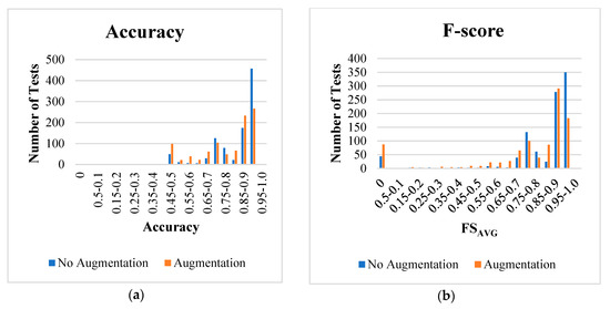
Figure 13.
Number of tests for accuracy (a) and f-score (b).
8. Conclusions
The loss in electricity production of the PV plant is significantly related to dirt, soiling or bird dejections deposited on the top surfaces of the modules. This paper proposes an innovative approach for the identification of possible abnormal operating conditions of PV systems using TNDTs supported by a CNN.
The CNN proposed is a high-performance software for the automatic recognition and classification of the thermographic images. It distinguishes hot spot conditions from those of dust, with an accuracy of 98% in tests 1, 2 and 9, in an interval of execution time between milliseconds to about 2 min, depending on the model and configuration chosen for the tests.
The rapidity and high accuracy of the tests allow one to highlight the factors that mainly contribute to a reduction in the electrical energy produced by the PV system. The use of TNDTs supported by RPA combined with the use of the CNN model proposed in the study enables a significant saving in terms of time required for the overall diagnostic procedure, especially in the case of inspection of large-size PV plants. Moreover, the utilization of RPA and open-source tools that use commodity hardware does not considerably increase the average annual maintenance costs of the PV systems, thereby making this approach affordable for many users.
In future works, new technologies for the detection of malfunctions in the operation of PV systems that use artificial intelligence will be evaluated, examining through TNDT the identification of cold spots, degenerative phenomena and the status of the wiring, including bypass diodes and junction boxes.
Author Contributions
Conceptualization, methodology, supervision of simulations and contributed to all draft: G.C., D.M., M.T. and V.D.D.; data curation: D.M.; software implementation, writing original draft preparation, writing review and editing A.D., S.G. and D.M. The contribution of the authors equally shared. All authors have read and agreed to the published version of the manuscript.
Funding
This research received no external funding.
Acknowledgments
The companies who provided thermographic images are as follows: SAIGE S.a.S., REA s.r.l., Andrea Carlini, Atlante snc.
Conflicts of Interest
The authors declare no conflict of interest.
Nomenclature
| A | accuracy (%) |
| b | bias vector of a fully connected layers network |
| annual electric output energy of the PV system (kWh/year) | |
| ReLU activation function | |
| FN | number of false negative samples |
| FP | number of false positive samples |
| estimated losses factor due to shadowing | |
| FS | f-score (%) |
| FSAVG | arithmetic means of the f-score values (%) |
| solar irradiance at the STC (W/m2) | |
| total annual solar irradiation on PV modules plan (kWh/(m2∙year)) | |
| loss factor including the presence of shading, mismatching, dust, soiling ed possible module failures | |
| N | number of tests |
| performance ratio of the PV system | |
| peak power of the PV system in STC (kWp) | |
| R | recall (%) |
| TN | number of true negative samples |
| TP | number of true positive samples |
| X | input vector of an activation function |
| Z | array containing the number of neurons of the previous layer and the current layer in a fully connected layers network |
| Greek letters | |
| azimuth angle of PV modules (°) | |
| tilt angle of PV modules (°) | |
| generic activation function of a fully connected layers | |
| Subscripts Abbreviations | |
| Aug | Augmentation techniques |
| C | False color image |
| CNN | Convolutional neural network |
| EMALS | Electromagnetic aircraft launch system |
| F | Box blur and Sobel–Feldman filters |
| G | Grayscaling |
| PV | Photovoltaic |
| SGD | Stochastic gradient descent |
| STC | Standard test conditions |
| TNDT | Thermographic non-destructive test |
References
- Colglazier, W. Sustainable development agenda: 2030. Science 2015, 349, 1048–1050. [Google Scholar] [CrossRef] [PubMed]
- GSE. Solare Fotovoltaico-Rapporto Statistico; GSE: Rome, Italy, 2018. [Google Scholar]
- Jäger-Waldau, A. Snapshot of Photovoltaics—February 2020. Energies 2020, 13, 930. [Google Scholar] [CrossRef]
- Nicolini, M.; Tavoni, M. Are renewable energy subsidies effective? Evidence from Europe. Renew. Sustain. Energy Rev. 2017, 74, 412–423. [Google Scholar] [CrossRef]
- European Union. E.U. Directive 2001/77/EC of the European Parliament and of the Council of 27 September 2001 on the Promotion of Electricity Produced from Renewable Energy Sources in the Internal Electricity Market. Off. J. Eur. Union 2001, 283, 82–209. [Google Scholar]
- Köntges, M.; Kurtz, S.; Packard, C.; Jahn, U.; Berger, K.A.; Kato, K.; Friesen, T.; Liu, H.; Iseghem, M.V.; Wohlgemuth, J.; et al. Review of Failures of Photovoltaic Modules; IEA: Paris, France, 2014. [Google Scholar]
- Photovoltaic Geographical Information System; European Communities: Paris, France, 2018.
- Pei, T.; Hao, X. A Fault Detection Method for Photovoltaic Systems Based on Voltage and Current Observation and Evaluation. Energies 2019, 12, 1712. [Google Scholar] [CrossRef]
- Ancuta, F.; Cepisca, C. Fault Analysis Possibilities for PV Panels. In Proceedings of the 3rd International Youth Conference on Energetics (IYCE), Bled, Slovenia, 3–6 July 2011; pp. 1–5. [Google Scholar]
- Musolino, A.; Raugi, M.; Rizzo, R.; Tucci, M. Optimal Design of EMALS Based on a Double-Sided Tubular Linear Induction Motor. IEEE Trans. Plasma Sci. 2015, 43, 1326–1331. [Google Scholar] [CrossRef]
- Jadin, M.S.; Taib, S. Recent progress in diagnosing the reliability of electrical equipment by using infrared thermography. Infrared Phys. Technol. 2012, 55, 236–245. [Google Scholar] [CrossRef]
- Cipriani, G.; Boscaino, V.; Di Dio, V.; Cardona, F.; Zizzo, G.; Di Caro, S.; Sa’Ed, J.A. Application of Thermographic Techniques for the Detection of Failures on Photovoltaic Modules. In Proceedings of the 2019 IEEE International Conference on Environment and Electrical Engineering and 2019 IEEE Industrial and Commercial Power Systems Europe (EEEIC/I&CPS Europe), Genova, Italy, 10–14 June 2019; pp. 1–5. [Google Scholar]
- Omar, T.; Nehdi, M.L. Remote sensing of concrete bridge decks using unmanned aerial vehicle infrared thermography. Autom. Constr. 2017, 83, 360–371. [Google Scholar] [CrossRef]
- Fenucci, D.; Caffaz, A.; Costanzi, R.; Fontanesi, E.; Manzari, V.; Sani, L.; Stifani, M.; Tricarico, D.; Turetta, A.; Caiti, A. WAVE: A Wave Energy Recovery Module for Long Endurance Gliders and AUVs. In Proceedings of the OCEANS 2016 MTS/IEEE, Monterey, CA, USA, 19–23 September 2016; pp. 1–5. [Google Scholar]
- Salazar, A.M.; Macabebe, E.Q.B. Hotspots Detection in Photovoltaic Modules Using Infrared Thermography. MATEC Web Conf. 2016, 70, 10015. [Google Scholar] [CrossRef]
- Ahmadipour, M.; Hazim, H.; Othman, M.L.; Radzi, M.A.M.; Chireh, N. A Fast Fault Identification in a Grid-Connected Photovoltaic System Using Wavelet Multi-Resolution Singular Spectrum Entropy and Support Vector Machine. Energies 2019, 12, 2508. [Google Scholar] [CrossRef]
- Zhao, Q.; Shao, S.; Lu, L.; Liu, X.; Zhu, H. A New PV Array Fault Diagnosis Method Using Fuzzy C-Mean Clustering and Fuzzy Membership Algorithm. Energies 2018, 11, 238. [Google Scholar] [CrossRef]
- Alsafasfeh, M.; Abdel-Qader, I.; Bazuin, B.; Alsafasfeh, Q.H.; Su, W. Unsupervised Fault Detection and Analysis for Large Photovoltaic Systems Using Drones and Machine Vision. Energies 2018, 11, 2252. [Google Scholar] [CrossRef]
- Bharath, K.V.S.; Blaabjerg, F.; Khan, M.A.; Haque, A. A Novel Fault Classification Approach for Photovoltaic Systems. Energies 2020, 13, 308. [Google Scholar] [CrossRef]
- Ji, D.; Zhang, C.; Lv, M.; Ma, Y.; Guan, N. Photovoltaic Array Fault Detection by Automatic Reconfiguration. Energies 2017, 10, 699. [Google Scholar] [CrossRef]
- Mani, M.; Pillai, R. Impact of dust on solar photovoltaic (PV) performance: Research status, challenges and recommendations. Renew. Sustain. Energy Rev. 2010, 14, 3124–3131. [Google Scholar] [CrossRef]
- Cristaldi, L.; Faifer, M.; Rossi, M.; Catelani, M.; Ciani, L.; Dovere, E.; Jerace, S. Economical Evaluation of PV System Losses Due to the Dust and Pollution. In Proceedings of the 2012 IEEE International Instrumentation and Measurement Technology Conference, Gratz, Austria, 13–16 May 2012; pp. 614–618. [Google Scholar]
- Teo, J.C.; Tan, R.H.G.; Mok, V.H.; Ramachandaramurthy, V.K.; Tan, C. Impact of Partial Shading on the P-V Characteristics and the Maximum Power of a Photovoltaic String. Energies 2018, 11, 1860. [Google Scholar] [CrossRef]
- Van Sark, W. Photovoltaic system design and performance. Energies 2019, 12, 1826. [Google Scholar] [CrossRef]
- Kudelas, D.; Taušová, M.; Tauš, P.; Gabániová, Ľ.; Koščo, J. Investigation of Operating Parameters and Degradation of Photovoltaic Panels in a Photovoltaic Power Plant. Energies 2019, 12, 3631. [Google Scholar] [CrossRef]
- Olalla, C.; Deline, C.; Maksimovic, D. Performance of Mismatched PV Systems with Submodule Integrated Converters. IEEE J. Photovolt. 2013, 4, 396–404. [Google Scholar] [CrossRef]
- Klugmann-Radziemska, E. Shading, Dusting and Incorrect Positioning of Photovoltaic Modules as Important Factors in Performance Reduction. Energies 2020, 13, 1992. [Google Scholar] [CrossRef]
- Goossens, D.; Offer, Z.; Zangvil, A. Wind tunnel experiments and field investigations of eolian dust deposition on photovoltaic solar collectors. Sol. Energy 1993, 50, 75–84. [Google Scholar] [CrossRef]
- Pavan, A.M.; Mellit, A.; De Pieri, D. The effect of soiling on energy production for large-scale photovoltaic plants. Sol. Energy 2011, 85, 1128–1136. [Google Scholar] [CrossRef]
- El-Shobokshy, M.S.; Hussein, F.M. Effect of dust with different physical properties on the performance of photovoltaic cells. Sol. Energy 1993, 51, 505–511. [Google Scholar] [CrossRef]
- Jiang, H.; Lu, L.; Sun, K. Experimental investigation of the impact of airborne dust deposition on the performance of solar photovoltaic (PV) modules. Atmos. Environ. 2011, 45, 4299–4304. [Google Scholar] [CrossRef]
- Klugmann-Radziemska, E.; Rudnicka, M. The Analysis of Working Parameters Decrease in Photovoltaic Modules as a Result of Dust Deposition. Energies 2020, 13, 4138. [Google Scholar] [CrossRef]
- Montes, C.; Gonzalez-Díaz, B.; Linares, A.; Llarena, E. Effects of the Saharan Dust Hazes in the Performance of Multi-MW PV Gridconnected Facilities in the Canary Islands (Spain). In Proceedings of the 25th European Photovoltaic Solar Energy Conference and Exhibition, Valencia, Spain, 6–10 September 2010; pp. 5046–5049. [Google Scholar]
- Zorrilla-Casanova, J.; Piliougine, M.; Carretero Rubio, J.E.; Bernaola-Galvan, P. Analysis of Dust Losses in Photovoltaic Modules. In Proceedings of the World Renewable Energy Congress-Sweden, Linköping, Sweden, 8–13 May 2011; pp. 2985–2992. [Google Scholar]
- Hassan, A.H.; Rahoma, U.A.; Elminir, H.K.; Fathy, A.M. Effect of airborne dust concentration on the performance of PV modules. J. Astron. Soc. Egypt 2005, 13, 24–38. [Google Scholar]
- Buerhop, C.; Scheuerpflug, H. Field Inspection of PV-Modules Using Aerial, Drone-Mounted Thermography. In Proceedings of the 29th European Photovoltaic Solar Energy Conference and Exhibition (EU PVSEC 2014), Amsterdam, The Netherlands, 22–26 September 2014; pp. 2975–2979. [Google Scholar]
- Parlevliet, D.A.; Urmee, T.; Parlevliet, D.A. PV system defects identification using Remotely Piloted Aircraft (RPA) based infrared (IR) imaging: A review. Sol. Energy 2020, 206, 579–595. [Google Scholar] [CrossRef]
- Buerhop, C.; Weißmann, R.; Scheuerpflug, H.; Auer, R.; Brabec, C.J. Quality Control of PV-Modules in the Field Using a Remote-Controlled Drone with an Infrared Camera. In Proceedings of the 27th European Photovoltaic Solar Energy Conference and Exhibition (EU PVSEC 2012), Frankfurt, Germany, 24–28 September 2012; pp. 3370–3373. [Google Scholar]
- IEC. IEC TS 62446-3-Photovoltaic (PV) Systems-Requirements for Testing, Documentation and Maintenance-Part 3: Photovoltaic Modules and Plants-Outdoor Infrared Thermography; IEC: Geneva, Switzerland, 2017. [Google Scholar]
- Gallardo-Saavedra, S.; Hernández-Callejo, L.; Duque-Perez, O. Technological review of the instrumentation used in aerial thermographic inspection of photovoltaic plants. Renew. Sustain. Energy Rev. 2018, 93, 566–579. [Google Scholar] [CrossRef]
- Grimaccia, F.; Aghaei, M.; Mussetta, M.; Leva, S.; Quater, P.B. Planning for PV plant performance monitoring by means of unmanned aerial systems (UAS). Int. J. Energy Environ. Eng. 2015, 6, 47–54. [Google Scholar] [CrossRef]
- Quater, P.B.; Grimaccia, F.; Leva, S.; Mussetta, M.; Aghaei, M. Light Unmanned Aerial Vehicles (UAVs) for Cooperative Inspection of PV Plants. IEEE J. Photovolt. 2014, 4, 1107–1113. [Google Scholar] [CrossRef]
- Spagnolo, G.S.; Vecchio, P.D.; Makary, G.; Papalillo, D.; Martocchia, A. A Review of IR Thermography Applied to PV Systems. In Proceedings of the 11th International Conference on Environment and Electrical Engineering, Venice, Italy, 18–25 May 2012; pp. 879–884. [Google Scholar]
- Ketkar, N. Introduction to Keras. In Deep Learning with Python; Springer: Berlin/Heidelberg, Germany, 2017; pp. 97–111. [Google Scholar]
- Dorobantu, L.; Popescu, M.O.; Popescu, C.L. Yield Loss of Photovoltaic Panels Caused by Depositions. In Proceedings of the 7th International Symposium on Advanced Topics in Electrical Engineering (ATEE), Bucharest, Romania, 7–9 May 2011; pp. 1–4. [Google Scholar]
- Ancuta, F.; Cepisca, C. Analysis of PV Panels Faults by Thermography. Proc. EVER Monaco 2011, 11–28, 128–134. [Google Scholar]
- Hopfield, J.J. Neural networks and physical systems with emergent collective computational abilities. Proc. Natl. Acad. Sci. USA 1982, 79, 2554–2558. [Google Scholar] [CrossRef] [PubMed]
- Pang, B.; Lee, L.; Vaithyanathan, S. Thumbs up? Sentiment classification using machine learning techniques. arXiv 2002, arXiv:cs/0205070. Available online: https://arxiv.org/abs/cs/0205070 (accessed on 4 December 2019).
- Krizhevsky, A.; Sutskever, I.; Hinton, G.E. ImageNet classification with deep convolutional neural networks. Commun. ACM 2017, 60. [Google Scholar] [CrossRef]
- Hubel, D.H.; Wiesel, T.N. Receptive fields of single neurones in the cat’s striate cortex. J. Physiol. 1959, 148, 574–591. [Google Scholar] [CrossRef] [PubMed]
- Lawrence, S.; Giles, C.L.; Tsoi, A.C.; Back, A.D. Face recognition: A convolutional neural-network approach. IEEE Trans. Neural Netw. 1997, 8, 98–113. [Google Scholar] [CrossRef] [PubMed]
- Xu, L.; Ren, J.S.J.; Liu, C.; Jia, J. Deep convolutional neural network for image deconvolution. Adv. Neural Inf. Process. Syst. 2014, 27, 1790–1798. [Google Scholar]
- Gardner, M.W.; Dorling, S.R. Artificial neural networks (the multilayer perceptron)—A review of applications in the atmospheric sciences. Atmos. Environ. 1998, 32, 2627–2636. [Google Scholar] [CrossRef]
- Estebon, M.D. Perceptrons: An Associative Learning Network. Spring. 1997. Available online: http://ei.cs.vt.edu/history/Perceptrons.Estebon.html (accessed on 20 September 2020).
- Jiang, X.; Pang, Y.; Li, X.; Pan, J.; Xie, Y. Deep neural networks with Elastic Rectified Linear Units for object recognition. Neurocomputing 2018, 275, 1132–1139. [Google Scholar] [CrossRef]
- Bera, S.; Shrivastava, V.K. Analysis of various optimizers on deep convolutional neural network model in the application of hyperspectral remote sensing image classification. Int. J. Remote Sens. 2019, 41, 2664–2683. [Google Scholar] [CrossRef]
- Lawrence, S.; Giles, C.L.; Tsoi, A.C. Lessons in Neural Network Training: Overfitting May Be Harder Than Expected. In Proceedings of the Fourteenth National Conference on Artificial Intelligence and Ninth Innovative Applications of Artificial Intelligence Conference, AAAI 97, IAAI 97, Providence, RI, USA, 27–31 July 1997; pp. 540–545. [Google Scholar]
- Li, Y.; Wang, J.; Zhao, H. Image Processing Method and Apparatus Using Self-Adaptive Binarization. U.S. Patent US7062099B2, 13 June 2006. [Google Scholar]
- Hummel, R.A.; Kimia, B.; Zucker, S.W. Deblurring Gaussian blur. Comput. Vis. Graph. Image Process. 1987, 38, 66–80. [Google Scholar] [CrossRef]
- Sobel, I.; Feldman, G. A 3x3 Isotropic Gradient Operator for Image Processing. In Pattern Classification and Scene Analysis; Wiley: New York, NY, USA, 1973. [Google Scholar]
- Mikolajczyk, A.; Grochowski, M. Data augmentation for improving deep learning in image classification problem. In Proceedings of the 2018 International Interdisciplinary PhD Workshop (IIPhDW), Świnoujście, Poland, 9–12 May 2018; pp. 117–122. [Google Scholar]
- Perez, L.; Wang, J. The effectiveness of data augmentation in image classification using deep learning. arXiv 2017, arXiv:171204621. Available online: https://arxiv.org/abs/1712.04621 (accessed on 20 December 2019).
- Forbes, A.D. Classification-algorithm evaluation: Five performance measures based onconfusion matrices. J. Clin. Monit. 1995, 11, 189–206. [Google Scholar] [CrossRef] [PubMed]


Publisher’s Note: MDPI stays neutral with regard to jurisdictional claims in published maps and institutional affiliations. |
© 2020 by the authors. Licensee MDPI, Basel, Switzerland. This article is an open access article distributed under the terms and conditions of the Creative Commons Attribution (CC BY) license (http://creativecommons.org/licenses/by/4.0/).