Abstract
The paper presents simulation research on a variable structure control scheme of a small variable-speed fixed-pitch wind energy conversion system (WECS) with a three-phase permanent magnet synchronous generator (PMSG) in variable wind conditions. The WECS is connected to a power grid through two back-to-back voltage source converters (VSCs) with a DC link. The presented control algorithm is based on feedforward compensation of the wind turbine aerodynamic torque estimated using a linear disturbance observer (DOB). The torque estimate is employed to determine the effective wind speed, required for setting the reference angular speed, using numerical zero search of a nonlinear function. The simulation model, built in the Matlab/Simulink environment using the Simscape Electrical toolbox, includes the field-oriented control of the PMSG via the machine VSC, performed by cascaded angular velocity and current/torque PI controllers, as well as synchronization with the grid and the reactive power control via the grid VSC. The presented results are focused on the performance of the proposed control in the maximum power point tracking (MPPT) operating region of the WECS for various wind speed profiles.
1. Introduction
Wind energy sources, along with solar energy sources, are considered to be the most promising renewable energy sources. Wind turbines (WTs) and wind power plants do not produce pollution or emissions, so wind energy conversion is one of the cleanest and safest methods for generating electricity. In 2019, wind energy provided an estimated 6% of the world’s and 15% of the EU’s annual electricity generation (47% in Denmark, the leading wind energy producer) [1]. Under the current rate of progress, wind energy will be able to meet about 29% of the world’s electricity consumption needs by 2030, with this figure reaching 34% by 2050. Falling costs per kilowatt-hour are making wind energy more and more competitive. However, due to the inherent variability of the wind, integration of wind power with the grid has brought various challenges, including power quality, system stability and planning. Contemporary wind energy conversion systems (WECSs) for the commercial production of electric power most often use WTs with horizontal rotational axis (HAWTs) and a three-blade rotor. In this work, we consider a Type 4 WECS, in which an induction or synchronous generator is connected to the grid through a full power converter [2]. Currently, permanent magnet synchronous generators (PMSGs) with back-to-back configuration of voltage source converters (VSCs) are widely used, especially in low-to-medium power WECSs. Their self-excitation property and lack of copper losses in the rotor circuit provide high power factor and efficiency. In WECSs with induction generators, the necessary reactive power has to be supplied through the converter. Neodymium magnets ensure high power density, so PMSGs are smaller in size, which reduces the cost and weight of WECSs. A great advantage of multipole direct-drive PMSG-based WECSs is that they operate at low speed, so the gearbox, one of the most unreliable mechanical components, is not necessary.
The design and control of contemporary WECSs allow for operation with variable rotational speed (VS). Large WTs are designed with variable-pitch rotor blades, and the pitch angle control is used at high wind speeds (above the WT nominal speed) to reduce the rotor speed and limit the captured power to the generator nominal power. Small WTs often have simpler construction with fixed pitch (so an actuator and mechanical system for pitch change are not required). The special design of blades results in a reduction of the aerodynamic torque above the nominal wind speed due to the stall effect (separation of the laminar airflow around a blade and occurrence of growing turbulence that spreads along a blade, induces drag forces and reduces the aerodynamic torque). Despite the simpler construction, at high wind speeds, passive stall-controlled WECSs have lower efficiency and undergo higher stresses [3].
From the control point of view, WECSs are nonlinear plants with nonlinear feedback, external disturbances and parameter uncertainties. On the other hand, optimal control of WECSs that maximizes the efficiency of electricity generation, especially in the partial-load operating region at low to medium winds, is of great long-term economic importance. It is estimated that more than 50% of annual energy output is obtained when a WECS operates in such a regime [4]. Therefore, to improve the control performance, researchers usually propose advanced nonlinear strategies of maximum power point tracking (MPPT). The most popular approaches in the literature are various versions of sliding mode control (SMC) like fuzzy SMC [5], integral SMC [6] or second-order SMC [7]. A comparison of several SMCs applied to WECS is presented in [8]. These (and many other) works show that SMC is an effective control technique ensuring stability and robustness to disturbances and parameter uncertainties. The known problems of SMC, like chattering or dealing with mismatched uncertainties, can be solved or reduced using higher-order or integral SMC, respectively, but in general, robustness is obtained at the cost of performance. Other model-based methods are backstepping [9] and model predictive control [10,11]. A different approach is the hill climb search (HCS) method, also known as the perturb and observe (P&O) approach. This method does not require knowledge of a plant model; it is based on perturbing the WT rotor speed and observing its impact on the output power [12].
Despite the advantages of the nonlinear techniques, many (if not most) WECS control systems are still based on linear or linearized models. The main reasons are that (1) this approach gives simpler analytical solutions to many control problems, like LQR/LQG or pole-zero placement, and (2) it is easier to implement controllers in practical applications. Even now, a significant part of WECSs (especially small WECSs) available on the market operate with controllers based on linearized models. The control based on linearizing (static) state feedback with PI and LQG controllers is presented in [13,14], respectively. An input–output feedback linearization with decoupling nonlinear variable transformation is proposed in [15]. Various versions of PI control are discussed in [16,17,18] (a scheme with the aerodynamic torque estimation and compensation), [19] (PI parameters varying with the wind speed), [20] (hybrid LQR-PI control) and [21] (PI with gain scheduling). Local linearization of a WT system model around an operating point is proposed in [22]. Principles and control design of WECS using linear parameter-varying (LPV) state-space models, whose dynamics vary as a function of certain time-varying scheduling parameters, are presented in [3,23].
Independent of a particular control technique, most MPPT algorithms rely on accurate effective wind speed, i.e., a mean wind speed on the whole WT rotor that generates the aerodynamic torque and is used to determine the command rotor angular velocity. An ultrasonic or cup anemometer installed on a WT nacelle measures the spot wind speed, which is disturbed by turbulence induced by the rotating rotor blades. Averaged measurement requires several anemometers placed at some distance from each other. Therefore, researchers have developed many techniques for effective wind speed estimation on the basis of other measured or estimated model variables. Reviews and comparisons of effective wind speed estimation methods are presented in [24,25]. Most commonly used methods are linear and nonlinear disturbance observers (DOBs) with numerical search of a nonlinear function zero (often referred to as the Newton–Raphson search) and estimators based on artificial intelligence techniques. Examples of the first approach are presented in the form of linear transfer function based DOBs in [17,26], Luenberger observers in [16,22], standard Kalman filters in [13,14,18] and adaptive Kalman filtering in [27]. The performance and robustness of the Takagi–Sugeno observer and a linear, extended (EKF) and unscented (UKF) Kalman filter are assessed in [28]. Effective wind estimators based on artificial intelligence are proposed in [16,29] (sigmoid MLP neural networks), [8] (ANFIS-based estimation) and [11] (support vector machine (SVM) and radial basis function (RBF) neural network with adaptation). An example of a different type of effective wind speed estimation, based on the power balance, is presented in [9].
This work presents a variable structure control scheme of a PMSG-based WECS with linearizing compensation of the aerodynamic torque considered as an input disturbance. Since the aerodynamic torque is unmeasurable, a linear DOB was employed to estimate the torque, both for the compensation and for the effective wind estimation using numerical search for finding a zero of a nonlinear function. The performance of the proposed scheme with PI controllers of the angular speed and the PMSG vector-controlled current/torque was verified by simulation in a wide range of wind speeds. The simulation model of the system, built in Simulink, includes a detailed model of the back-to-back VSCs connected to a power grid. The research is focused on the performance of the WECS model in the MPPT operating region in variable wind speed conditions, but results for full-load operation at high winds above the MPPT region are also presented. Electrical phenomena occurring on the WECS–grid connection, like voltage dips or short circuits, are not considered, so the simulation model does not satisfy some standard requirements [30]. A similar control scheme based on compensation using the aerodynamic torque estimate, but with a different wind speed estimation method, is presented in [16].
2. WECS System Configuration
The considered WECS scheme is presented in Figure 1. The system is composed of a small HAWT that is directly coupled with a slow-speed multipole PMSG connected to a power grid through back-to-back power converters. The sensors present in the scheme are an optical encoder for the measurement of the rotor velocity ω and the phase current and voltage (only on the grid side) sensors.
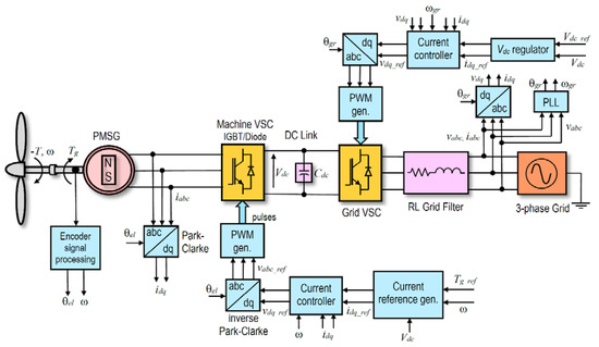
Figure 1.
Configuration of a gearless permanent magnet synchronous generator (PMSG)-based wind energy conversion system (WECS) connected to a grid through back-to-back voltage source converters (VSCs) with schematic block diagram of the converters’ control.
3. Wind Power Extraction
The aerodynamic power that a wind turbine captures from the wind is expressed as follows:
where R is the blade tip radius (A = πR2 is the rotor swept area), ρ is the air density, v is the effective wind speed and Cp is the power coefficient that specifies the power conversion efficiency (Cp < 1).
For a fixed-pitch wind turbine, the power coefficient is a function of a single variable, i.e., the tip-speed ratio (TSR), defined as
where ω is the turbine shaft angular velocity. The power coefficient is limited by the theoretical Betz limit: any type of wind turbine (also with a vertical axis) cannot capture more than 16/27 = 0.593 of the wind kinetic energy. Practical utility-scale HAWTs achieve at peak Cp ≈ 0.45 [3]. The mechanical (aerodynamic) torque developed by the turbine is
If we denote
The power coefficient curve Cp(λ) is generally determined experimentally and provided by the turbine manufacturer. An experimental dataset for a small fixed-pitch wind turbine and a corresponding function curve fitting are shown in Figure 2. In general, the power coefficient curves have one maximum Cpmax, which means that for a given effective wind speed v the maximum aerodynamic power is captured for some optimal tip-speed ratio λopt. This is the basis for optimal control of WECSs at low-to-medium winds.
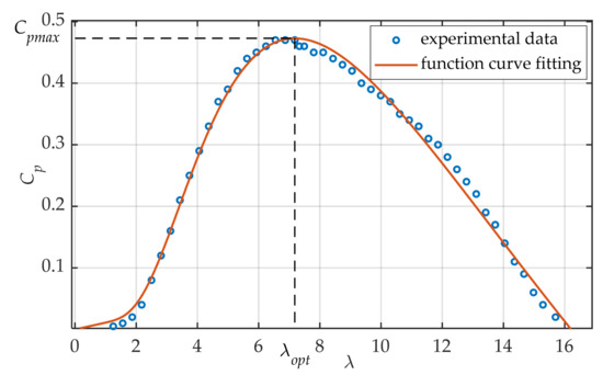
Figure 2.
Experimental power coefficient data points and the corresponding function curve fitting using Function (5). Data provided by courtesy of MMB Drives Sp. z o.o., Gdańsk, Poland.
For further analysis and control design, the approximating function (proposed in [31,32])
was fitted to the data points with the following coefficients: β = 0 (this is the pitch angle in degrees for variable-pitch WTs; for a fixed-pitch WT, it is set to zero), c1 = 0.23, c2 = 104.5, c3 = 0.4, c4 = 33.9, c5 = 13.5 and c6 = 0.011. For these parameters, λopt = 7.18 and Cpmax = 0.47.
Operation and control modes of a WECS with wind speed growth are usually divided into four regions. The basic characteristics of a WECS mechanical output power versus the wind speed are shown in Figure 3. Region 1 is a spin-up zone without energy conversion, because the wind is too low. When the wind speed exceeds the cut-in speed vcut-in (usually 4–5 m/s for small WTs), the energy conversion is started and the WT speed is controlled using the generator torque so that the maximum possible power is captured at each wind speed according to the turbine characteristics. The captured power is proportional to the third power of the wind speed as in formula (1). The partial-load region 2 extends to the wind speed at which the generator achieves its nominal angular speed ωgn. Usually, this wind speed vωgn is lower than the WT nominal wind speed vn so, in the transition region 3, the captured power still increases with the second power of the wind speed, but the control system limits the WECS speed to ωgn and the power capture is below optimal. When the wind achieves nominal speed vn, the WT mechanical output reaches nominal power Pn. The nominal wind speed of onshore WTs is typically between 10 and 12 m/s. In the full-load region 4, above the nominal wind speed, the WT is controlled so that the produced power is limited to Pn at a maximum acceptable angular speed either by increasing the pitch angle (in variable-pitch WTs) or due to the stall effect (in fixed-pitch WTs). Above a specified cut-out wind speed vcut-out, the WECS is shut down to prevent structural overload. Onshore HAWTs are designed to operate at wind speeds up to 20–25 m/s. In all of the regions, the control should not produce undesirable mechanical loads of the WECS, like fast changes of the generator torque.
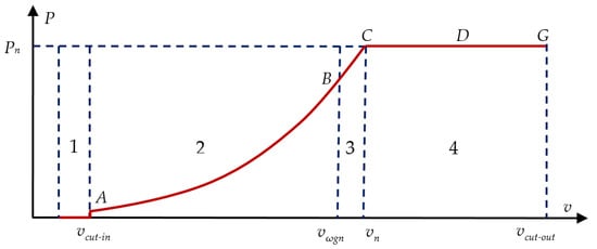
Figure 3.
Basic operating characteristic of a wind turbine (WT) mechanical output power versus the wind speed divided into operating regions.
Figure 4 presents a typical characteristic of the rotor velocity of a variable-speed fixed-pitch (VSFP) stall-regulated WT versus the wind speed over the operating regions. In region 2, rotor velocity ω grows linearly with v to preserve the optimal TSR, i.e., ω = λoptv; in region 3, it is kept constant, i.e., ω = ωgn; and in region 4, it has to be reduced so as not to exceed nominal power Pn. Interval DG denotes operation in the stall area, where the aerodynamic torque is reduced due to the stall effect [3].
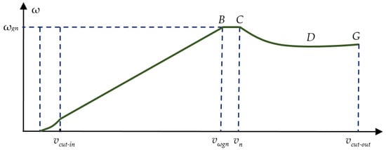
Figure 4.
Typical characteristic of the rotor velocity versus the wind speed over the operating regions marked in Figure 3 for a variable-speed fixed-pitch (VSFP) WT.
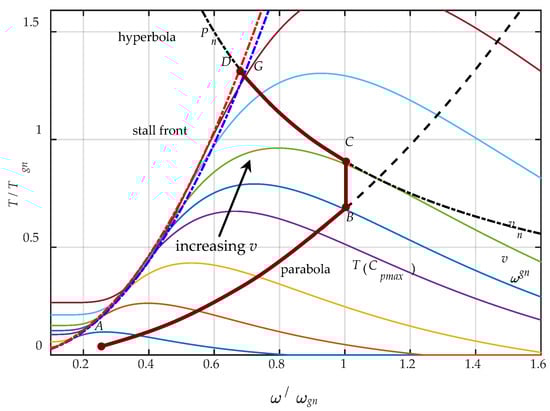
The curve ABCDG in Figure 5 is the trajectory drawn by operating points of a VSFP WT on the ω–T plane for increasing wind speed and the power and rotational speed control strategy depicted in Figure 3 and Figure 4. The per-unit scale values are for the ratio of the turbine and the generator nominal power Pn/Pgn = 0.9. The turbine maximum power (i.e., P(Cpmax)) at the nominal wind speed vn is nominal power Pn, the rotor velocity at this maximum power is ω = 1.1ωgn and Tgn = Pgn/ωgn. These data are the input parameters for the wind turbine block in Simulink [32]. The family of T(ω) curves for different wind speed v was plotted using Function (5).
4. WECS Model Description
4.1. Permanent Magnet Synchronous Generator
It is assumed that that the considered three-phase PMSG is the surface-mounted magnets type with nonsalient poles and sinusoidal back-EMF waveform. The phase equations of the generator stator transformed to the d–q reference frame rotating with angular velocity ω of the rotor using the Park–Clarke transform (applied to measured PMSG phase currents ia, ib, ic) take the following form [33]:
where Ld and Lq are stator (armature) inductances in d–q axes, R is stator resistance and ψPM is constant flux induced by the rotor permanent magnets in the stator phases (flux linkage); ωe= npω and is the electrical angular velocity, where np is the number of pole pairs.
In a steady state, the voltages and currents in the rotating reference frame are constant.
Equation (6) includes cross-coupling speed voltages ωeLqiq and ωeLdid. These terms, as well as the flux linkage term ωeψPM, will be compensated in the current controller to obtain two decoupled first-order inertia circuits that are easy to control. In general, the electromagnetic torque developed by a PMSG generator
consists of two components: the PM torque and the reluctance torque that is generated in machines with salient poles. In the considered PMSG, the stator inductances in the perpendicular axes are equal, i.e., Ld = Lq, and the torque is the function of only one variable, i.e., the current in q-axis:
where kT = 1.5npψPM is the torque constant. To reduce the total current and optimize operating conditions, the machine should be controlled so that the d-axis current is zero.
4.2. Voltage Source Converters
Electric power produced by the PMSG is transferred to the power grid through two three-phase full-bridge two-level PWM voltage source converters in the back-to-back configuration with a DC link as shown in Figure 1. The machine-side converter (MSC) operates as a rectifier, whose PWM pulses are provided by the proposed controllers and perform a vector (field-oriented) control of the PMSG. The grid-side converter (GSC) operates as an inverter, whose role is to transfer the energy stored in the DC link to the grid. The GSC controller stabilizes voltage Vdc on the DC link and synchronizes (using the phase-locked loop (PLL)) and controls the GSC output voltages and currents to establish an appropriate grid connection [34].
4.3. Mechanical Model
The equations of the electrical subsystem (6) and (8) have to be supplemented by an equation of the WECS’s mechanical subsystem. It is assumed that, in the case of a small wind turbine, the elasticity of the shaft can be neglected and an adequate description is the one-mass dynamical model:
where J is the total moment of inertia of the wind turbine coupled with the PMSG and B is the total coefficient of the viscous friction. The one-mass model was also used in [5,6,13,16,20,26,29]. In [18], we employed a two-mass drivetrain model with a simple first-order inertia dynamics of the electrical subsystem.
5. Control Scheme
The proposed control scheme for a WECS with one-mass mechanical model and functional approximation of the power coefficient curve is shown in Figure 6.
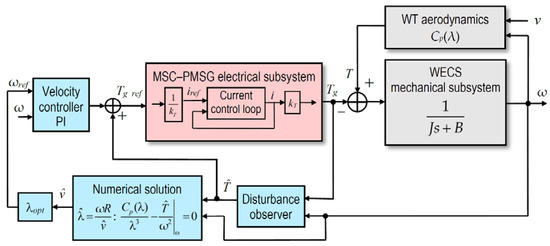
Figure 6.
Proposed maximum power point tracking (MPPT) control scheme for a WECS with one-mass mechanical model and functional approximation of the power coefficient curve. The details of the angular velocity and the current/torque controllers are shown in Figure 9.
The role of the disturbance observer is to estimate the wind turbine aerodynamic torque on the basis of measured rotor velocity ω and the generator torque (8) using the scheme presented in Figure 7 (see also [17,26]). Gm(s) is a model of the wind turbine transfer function G(s), and P(s) is a unit gain coefficient lowpass filter of the relative order high enough to make the transfer function P(s)/Gm(s) realizable. Then,

Figure 7.
Transfer function based disturbance observer.
If the model is accurate, i.e., Gm(s) = G(s), and T→const, then →T for t→∞ [35]. However, the estimation is also effective when T varies slowly compared to the lowpass filter time constant Tdob, which is the DOB parameter and should be set much lower than the periods of the wind speed variations. For the first-order G(s) resulting from (9), we selected a second-order filter
with Tdob = 0.05 s and damping factor ζ = 1.
The estimate of the wind speed is obtained as a solution of a numerical search for roots of a nonlinear function. If we assume that the torque estimate is accurate, i.e.,
then the problem is reduced to finding zeros of the nonlinear function of tip-speed ratio λ:
where Cp(λ) is the functional approximation (5) of the power coefficient experimental curve. The problem is illustrated in Figure 8. The correct solution lies on the right-hand side descending part of the function. There are two or three roots in the stall area marked in Figure 5, where Equation (3) loses validity due to turbulence. The left-hand side of the plot depends strongly on a particular approximating function. The wind speed estimate is obtained directly as .
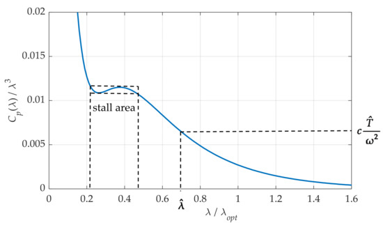
Figure 8.
Finding roots of the nonlinear function, c = 2/(πρR5).
A more detailed scheme of the cascaded rotor velocity and current controllers is presented in Figure 9. The use of proportional–integral (PI) controllers is a well-established solution for field-oriented control of electric machines. It is particularly justified in combination with linearizing feedback or disturbance rejection, like the aerodynamic torque compensation proposed in this article. This solution is simple and usually ensures better performance than, e.g., nonlinear sliding mode control, at some cost of robustness. Its effectiveness in the context of WECS with three-phase full-bridge PWM controlled generators has often been demonstrated [13,16,19,20]. The linearizing feedforward compensation of the aerodynamic torque was earlier employed in [16,17,26].
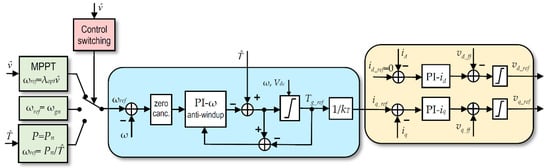
Figure 9.
Rotor velocity and current controllers with variable structure setting of ωref and compensation input of aerodynamic torque estimate .
The inner loop current controllers perform the maximum torque per ampere (MTPA) control [33]. Therefore,
The feedforward compensating voltage components
added to the output (note that vd_ff is added with minus in Figure 9) decouple current control in d–q axes. For a PM machine with nonsalient poles, Ld = Lq = L, and the PI-i parameters are set the same in both axes. The parameters of the PI-i transfer function
were designed to cancel the electrical time constants L/R of the generator stator circuit and obtain the current control closed loop of the following form:
where ωcc is a design parameter. This requirement is satisfied when the current PI parameters are set as
The bandwidth of the current loop was set to fcc = ωcc/2π = 100 Hz, which is 1/30 of the converters’ switching frequency fsw=3000 Hz.
The open-loop transfer function of the speed control system with the inner current control loop is
Following [33], the crossover frequency ωcω of this open-loop, which is close to the velocity control closed-loop bandwidth, should be selected as much smaller than the current control bandwidth ωcc so that for ωcω the current loop dynamics is negligible (i.e., |GcCL(jωcω)|≈ 1). Taking into account that the wind turbine inertia constant (see parameters in Table 1)
we selected ωcω = 2 rad/s, which corresponds to the velocity control closed-loop time constant Tω ≈ 0.5 s. Finally, the PI-ω corner frequency ωpi = kiω/kpω was selected as ωpi = ωcω/3 (giving a phase margin PM ≈ 75°) to obtain a relatively fast dynamic response. The velocity controller settings are given as follows:

Table 1.
Wind turbine parameters.
In addition, the velocity controller includes a variable level reference torque limiter, integrator anti-windup loop and a zero-cancellation filter
that cancels the PI-ω controller zero, thus reducing the velocity response overshoot.
6. Simulation Model
The simulation model was built in Simulink, version 2020a, using the wind turbine block and three-phase blocks from the Simscape Electrical Toolbox: the PMS machine and universal bridge for the VSCs, series RLC branch for the grid filter and series RLC load and programmable voltage source for the grid and V-I measurement blocks. The GSC control and the current control of the MSC were based on a detailed model [36], available online, with minor modifications. The model is a pure discrete-time system, so the Laplace transfer functions presented in previous sections were discretized to the corresponding Z transfer functions and the discrete-time PI controller blocks were used.
Physical parameters of the model are presented in Table 1, Table 2 and Table 3. For simulation, most parameters were scaled to per-unit values. The fundamental simulation step size was set to 5 μs, but the observer and the controllers’ outputs were updated every 100 μs, which is equal to one typical PWM control cycle in practical applications. In real-time implementations, the period of the wind speed estimate computation and the rotor velocity control update can be much longer, of the order of 100 ms.
Table 2.
PMSG parameters.
Table 3.
DC link, VSCs and grid parameters.
Matlab function fzero, which uses a combination of bisection, secant and inverse quadratic interpolation methods, was used for finding zeros of Function (13) in each control cycle.
The three-phase V-I measurement block from the Simscape Electrical Toolbox allows measuring instantaneous three-phase voltages and currents at a given point of a three-phase circuit. These measurements can be used to calculate active and reactive electric power at this point as
where ia, ib and ic are the phase currents; va, vb and vc are the phase-to-ground voltages; and vab, vbc and vca are the phase-to-phase voltages.
7. Results
Figure 10 shows plots of the WECS variables for a theoretical step-change wind speed within the MPPT region. This simulation was carried out to present the dynamic performance of the proposed MSC control. One can see the fast performance of the disturbance observer (Test is the aerodynamic torque estimate) and the errorless computation of the wind speed estimate vest. The angular speed response has no overshoot. However, the fast speed response requires rapid changes in the actuating generator torque. Potential excessive mechanical loads may be avoided by reducing crossover frequency ωcω (a design parameter, see Section 6) and slowing down the speed response. At steady states, the WECS operates at maximum power points Cp = Cpmax. The GSC control blocks the inductive reactive power generated by the PMSG—the mean reactive power Q transferred to the grid is about zero.
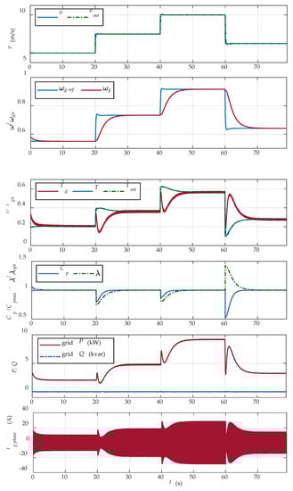
Figure 10.
Plots of the WECS variables for theoretical step-change wind speed profile 6→8→10→7 m/s. P and Q denote mean active and reactive power at the grid side of the RL filter (see Figure 1), Tgn = 1910 Nm and ig_phase shows the envelope of the PMSG variable-frequency phase current.
The operation of the WECS for a more realistic wind speed profile with a slowly varying sine component and rapid random gusts is presented in Figure 11.
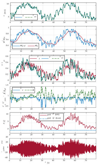
Figure 11.
Plots of the WECS variables for the wind speed profile with slowly varying sine components and superimposed random noise, described by Formula (21).
The formula used in the simulation for the wind speed was
where n(t) is a zero-mean band-limited white noise.
The angular speed follows the slowly varying sine component due to the high inertia of the turbine–generator coupling, but a much faster current/torque control loop tries to react to fast random changes of the aerodynamic torque. There are no wind speed estimation errors, and the WECS oscillates around the maximum power operating point at all times. As in the previous example, the GSC control keeps the mean reactive power Q transferred to the grid at zero.
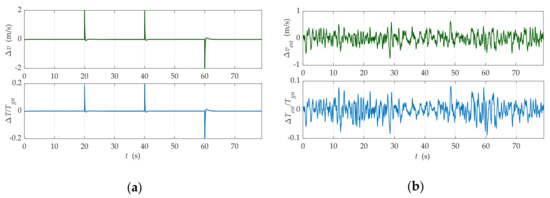
The estimation errors of the wind speed and the aerodynamic torque for the WECS operation examples shown in Figure 10 and Figure 11 are plotted in Figure 12.
The third example presents the WECS response to a single coherent wind gust, which is one of the standard test wind profiles described in [37]. The gust in Figure 13 has a 3-s rising slope from 6 to 10 m/s, 12-s flat sector and a longer 6-s falling slope.
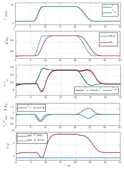
Figure 13.
Plots of the WECS variables for a single coherent wind gust.
The performance of the WECS over the entire range of operating conditions, i.e., regions 2, 3 and 4, is presented in Figure 14 for slowly, linearly increasing wind speed. It allows for comparison of the WECS state changes with the static characteristics of a fixed-pitch stall-regulated WT shown in Figure 4 and Figure 5. Since time is proportional to the wind speed, the plot of angular speed ω in Figure 14 is close to the corresponding characteristic of ω versus v from Figure 4. Similarly, the trajectory drawn by the WT state variables (ω,T) in Figure 15 is close to the static characteristic in Figure 5.
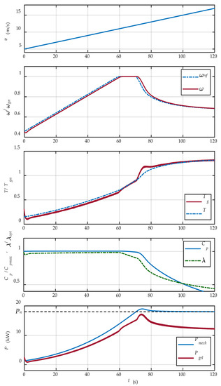
Figure 14.
Plots of the WECS variables for the wind speed slowly, linearly growing with the slope 0.1 m/s2.
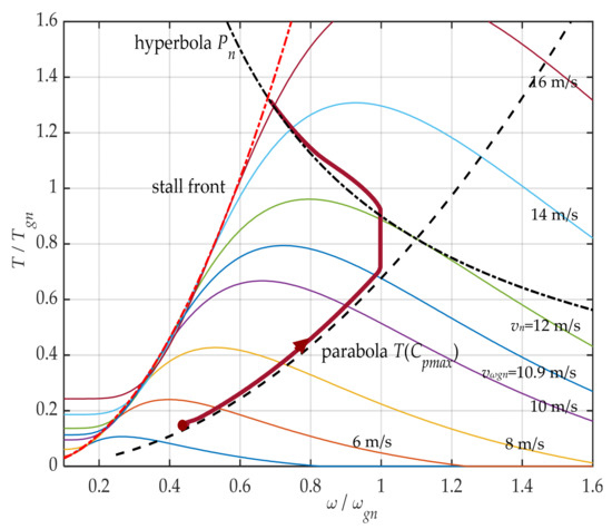
Figure 15.
Quasi-static trajectory drawn by the WT state variables (ω,T) for the linearly increasing wind speed profile shown in Figure 14.
8. Discussion
For a better assessment of the proposed control scheme performance, it was compared with conventional indirect torque control (compare Formula (4))
based on the intrinsic stability of a wind turbine that converges to the maximum power point under this control. The indirect torque control is a soft control that might be useful for small low-inertia WTs. The results of the comparison for the coherent gust are presented in Figure 16. One can see that the proposed control is faster and the transient deviations from the maximum power point are shorter and smaller. However, faster acceleration under increasing wind speed is obtained by reducing the generator toque (faster deceleration under decreasing wind is obtained by increasing the generator torque), which has the opposite effect on the amount of generated electrical energy.
Tg_ref = Koptω2, where Kopt = ½πρCpmax/λopt
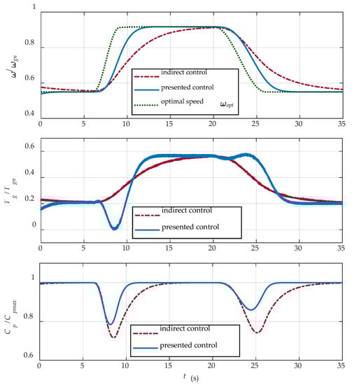
Figure 16.
Comparison of the proposed control with conventional indirect torque control; ωopt = λoptv/R.
Integration of the waveforms of generated active power P(t) produced the following results:
- The proposed MPPT control gave 1.5% more electrical energy than the indirect torque control for the considered sine-random wind profile;
- The proposed MPPT control gave 3.1% more electrical energy than the indirect torque control for the considered coherent gust.
Certainly, it is not reasonable to generalize the presented results, but the proposed scheme with feedforward disturbance compensation has been widely applied in control applications. Even though in the WECS case, the MSC-PMSG electrical subsystem appears between the compensation input and disturbance input (Figure 6), its dynamics is much faster (the designed current control loop bandwidth fcc = 100 Hz) than that of the mechanical subsystem and has a negligible impact. Another important advantage of the aerodynamic torque compensation is the linearization of the plant. One piece of evidence is the plot of angular speed ω in Figure 10, where the speed step response is the same for the low wind and for the high wind. Linearization makes it possible to use existing feedback control methods like simple PID controllers. In general, the disturbance observer-based compensation is added to improve the robustness and disturbance attenuation of the main controller. This approach is an effective technique and does not have the weakness of robust control methods, in which the control is in principle “conservative” and the robustness is achieved at the price of degraded nominal performance.
If we omit the MSC and GSC current control and the PWM pulse generation, which are typically performed by dedicated embedded microcontrollers or FPGAs, the most time-consuming part of the control algorithm is numerical search for the effective wind speed estimate. In the case of nonlinear Equation (13), a single step required from 3 to 13 iterations of the bisection procedure and from 8 to 37 computations of Cp(λ) Function (5) for the search termination tolerance 10−4. The corresponding computation time of a single search varied from 0.5 to 5 ms on a PC with a processor whose computing capacity is comparable with that of, e.g., the inexpensive and popular Raspberry Pi 4B (with ARM Cortex A72, 1.5 GHz, 64-bit quad-core processor). It is fast enough for the real-time implementation of the algorithm part that computes the PMSG reference torque/current for the MSC microcontroller if the update period of the wind speed estimate and this reference torque is 20 to 100 ms, which is a reasonable choice taking into account that the WT inertia constant (17) is 2.8 s. The Raspberry Pi board could also be a good candidate for another reason: it is supported by Simulink as a hardware platform, so the target code can be generated directly from the Simulink block diagram.
9. Conclusions
Even though the components of the presented control scheme are known and have already been employed in control studies and applications, the contributions of this research are as follows:
- Systematic description of the control design, i.e., dynamic estimation of the aerodynamic torque and numerical computation of the effective wind speed, the rotor velocity control loop and the inner current control loop, using the model with a detailed scheme of the electrical subsystem with back-to-back converters;
- Simulation verification and presentation of the very good control dynamic quality in the form of the responses to the step-change wind profile (Figure 10) and to the coherent wind gust (Figure 13); the most common forms of a WECS control presentation in the literature, especially for simulation studies of nonlinear control strategies, are plots for random wind speed profiles, which makes it difficult to assess and compare the dynamic performance of the control;
- Demonstration that the presented control exhibits better wind power capturing efficiency (in the MPPT region) than the indirect torque control (22) for the random wind speed profile as well as for the coherent gust (Figure 16).
Almost the same control scheme with the aerodynamic torque compensation is proposed in [16]. A Luenberger observer is used for estimation of the aerodynamic torque and a neural network for the wind speed estimation. The authors validate the variable structure control experimentally on a test rig over the whole wind speed range, but they show only quasi-static characteristics like those in Figure 14 and Figure 15 here. A simulation study similar to this work is presented in [15], where the authors discuss a feedback linearization of a PMSG-based WECS, but the wind speed estimation is omitted and the rotor speed response to the wind step-change on the presented plots takes less than one second (for a 2 MW WT!).
Further research will go towards the development and verification of the proposed approach by using more detailed models of the mechanical subsystem, including the FAST model, and validation of the simulation model on a laboratory-scale experimental WECS setup.
Author Contributions
Conceptualization, J.B. and A.J.; methodology, J.B. and A.J.; software, J.B.; validation, J.B.; investigation, J.B.; writing—original draft preparation, J.B.; writing—review and editing, J.B.; visualization, J.B.; supervision, A.J. All authors have read and agreed to the published version of the manuscript.
Funding
This research received no external funding.
Acknowledgments
The authors would like to acknowledge the MMB Drives Sp. z o.o. company, Gdańsk, Poland, for making available experimental data.
Conflicts of Interest
The authors declare no conflict of interest.
Abbreviations
| DOB | disturbance observer |
| FOC | field-oriented control |
| FP WT | fixed-pitch wind turbine |
| GSC | grid side converter |
| HAWT | horizontal axis wind turbine |
| HCS | hill climb search |
| MPPT | maximum power point tracking |
| MSC | machine side converter |
| MTPA | maximum torque per ampere |
| PLL | phase-locked loop |
| PMSG | permanent magnet synchronous generator |
| PWM | pulse width modulation |
| SMC | sliding mode control |
| TSR | tip-speed ratio |
| VSC | voltage source converter |
| VS WT | variable-speed wind turbine |
| WECS | wind energy conversion system |
| WT | wind turbine |
References
- Renewables 2020 Global Status Report. Available online: https://www.ren21.net/reports/global-status-report/ (accessed on 21 October 2020).
- Wu, Q.; Sun, Y. (Eds.) Modeling and Modern Control of Wind Power; John Wiley & Sons: Chichester, UK, 2018. [Google Scholar]
- Bianchi, F.; De Battista, H.; Mantz, R. Wind Turbine Control Systems. Principles, Modelling and Gain Scheduling Design; Springer: London, UK, 2007. [Google Scholar]
- Johnson, K.; Fingersh, L.; Balas, M.; Pao, L. Methods for Increasing Region 2 Power Capture on a Variable Speed HAWT. In Proceedings of the 42nd AIAA Aerospace Sciences Meeting and Exhibit, Reno, NV, USA, 5–8 January 2004. [Google Scholar] [CrossRef]
- Do, T.D. Disturbance observer-based fuzzy SMC of WECSs without wind speed measurement. IEEE Access 2016, 5, 147–155. [Google Scholar] [CrossRef]
- Watil, A.; El Magri, A.; Raihani, A.; Lajouad, R.; Giri, F. Multi-objective output feedback control strategy for a variable speed wind energy conversion system. Int. J. Electr. Power Energy Syst. 2020, 121. [Google Scholar] [CrossRef]
- Beltran, B.; Benbouzid, E.H.M. Second-order sliding mode control of a doubly fed induction generator driven wind turbine. IEEE Trans. Energy Convers. 2012, 27, 261–269. [Google Scholar] [CrossRef]
- Golnary, F.; Moradi, H. Dynamic modelling and design of various robust sliding mode controls for the wind turbine with estimation of wind speed. Appl. Math. Model. 2018. [Google Scholar] [CrossRef]
- Majdoub, Y.; Abbou, M.; Akherraz, M. Variable speed control of DFIG-wind turbine with wind estimation. In Proceedings of the 3rd International Renewable and Sustainable Energy Conference, Marrakech, Morocco, 10–13 December 2015. [Google Scholar] [CrossRef]
- Song, D.; Yang, J.; Dong, M.; Joo, Y.H. Model predictive control with finite control set for variable-speed wind turbines. Energy 2017, 126, 564–572. [Google Scholar] [CrossRef]
- Li, D.-Y.; Cai, W.-H.; Li, P. Neuro-adaptive variable speed control of wind turbine with wind speed estimation. IEEE Trans. Ind. Electron. 2016, 63, 7754–7764. [Google Scholar] [CrossRef]
- Yaakoubi, A.E.; Amhaimar, L.; Attari, K.; Harrak, M.; Halaoui, M.; Asselman, A. Non-linear and intelligent maximum power point tracking strategies for small size wind turbines: Performance analysis and comparison. Energy Rep. 2019, 5, 545–554. [Google Scholar] [CrossRef]
- Boukhezzar, B.; Siguerdidjane, A. Nonlinear control with wind speed estimation of a DFIG variable speed wind turbine for power capture optimization. Energy Convers. Manag. 2009, 50, 885–892. [Google Scholar] [CrossRef]
- Boukhezzar, B.; Siguerdidjane, A. Comparison between linear and nonlinear control strategies for variable speed wind turbines. Control. Eng. Pract. 2010, 18, 1357–1368. [Google Scholar] [CrossRef]
- Chen, J.; Jiang, L.; Yao, W.; Wu, Q.H. A feedback linearization control strategy for maximum power point tracking of a PMSG based wind turbine. In Proceedings of the 2013 International Conference on Renewabl Energy Research and Applicatioms, Madrid, Spain, 20–23 October 2013; pp. 79–84. [Google Scholar] [CrossRef]
- Calabrese, D.; Tricarico, G.; Brescia, E.; Cascella, G.L.; Monopoli, V.G.; Leuzzi, R. Variable Structure Control of a Small Ducted Wind Turbine in the Whole Wind Speed Range Using a Luenberger Observer. Energies 2020, 13, 4647. [Google Scholar] [CrossRef]
- Baran, J.; Jąderko, A. Układ sterowania turbiny wiatrowej o regulowanej prędkości obrotowej i stałym kącie ustawienia łopat z liniowym obserwatorem momentu aerodynamicznego. Prz. Elektrotech. 2017, 93, 59–62. (In Polish) [Google Scholar] [CrossRef]
- Baran, J.; Jąderko, A. Sterowanie turbiną wiatrową z odtwarzaniem momentu aerodynamicznego. Prz. Elektrotech. 2018, 94, 47–52. (In Polish) [Google Scholar] [CrossRef]
- Kim, J.-S.; Chung, I.-Y.; Moon, S.-I. Tuning of the PI controller parameters of a PMSG wind turbine to improve control performance under various wind speeds. Energies 2015, 8, 1406–1425. [Google Scholar] [CrossRef]
- Kim, K.; Kim, H.-G.; Song, Y.; Paek, I. Design and simulation of an LQR-PI control algorithm for medium wind turbine. Energies 2019, 12, 2248. [Google Scholar] [CrossRef]
- Song, D.; Yang, J.; Cai, Z.; Dong, M.; Su, M.; Wang, Y. Wind estimation with a non-standard extended Kalman filter and its application on maximum power extraction for variable speed wind turbines. Appl. Energy 2017, 170, 670–685. [Google Scholar] [CrossRef]
- Munteanu, I.; Basançon, G. Control-based strategy for effective wind speed estimation in wind turbines. In Proceedings of the 19th World IFAC Congress—IFAC, Cape Town, South Africa, 24–29 August 2014; pp. 6776–6781. [Google Scholar] [CrossRef]
- Trilla, L.; Bianchi, F.D.; Gomis-Bellmunt, O. Linear parameter-varying control of PMSGs for wind power systems. IET Power Electron. 2014, 7, 692–704. [Google Scholar] [CrossRef]
- Jena, D.; Rajendran, S. A review of estimation of effective wind speed based control of wind turbines. Renew. Sustain. Energy Rev. 2014, 43, 1046–1062. [Google Scholar] [CrossRef]
- Soltani, M.N.; Knudsen, T.; Svenstrup, M.; Wisniewski, R.; Brath, P.; Ortega, R.; Johnson, K. Estimation of Rotor Effective Wind Speed: A Comparison. IEEE Trans. Control. Syst. Technol. 2013, 21, 1155–1167. [Google Scholar] [CrossRef]
- Hu, Z.; Wang, J.; Ma, Y.; Yan, X. Research on speed control system for fixed-pitch wind turbine based on disturbance observer. In Proceedings of the 2009 World Non-Grid-Connected Wind Power and Energy Conference, Nanjing, China, 24–26 September 2009; pp. 221–225. [Google Scholar] [CrossRef]
- Bourlis, D. Control Algorithms and Implementation for Variable Speed Stall Regulated Wind Turbines. Ph.D. Thesis, University of Leicester, Leicester, UK, 2010. [Google Scholar]
- Gauterin, E.; Kammerer, P.; Kühn, M.; Schulte, H. Effective wind speed estimation: Comparison between Kalman filter and Takagi–Sugeno observer techniques. ISA Trans. 2016, 62, 60–72. [Google Scholar] [CrossRef] [PubMed]
- Qiao, W.; Yang, X.; Gong, X. Wind speed and rotor position sensorless control for direct-drive PMG wind turbines. IEEE Trans. Ind. Appl. 2012, 48, 3–11. [Google Scholar] [CrossRef]
- International Electrotechnical Commission—IEC. IEC 61400-27-1. Electrical Simulation Models-Wind Turbines; IEC: Geneva, Switzerland, 2015. [Google Scholar]
- Heier, S. Grid Integration of Wind Energy Conversion Systems; John Wiley & Sons: Chichester, UK, 1998. [Google Scholar]
- Hydro-Quebec. Simscape Electrical Reference (Specialized Power Systems); The Mathworks Inc.: Natick, MA, USA, 2019. [Google Scholar]
- Kim, S.-H. Electric Motor Control. DC, AC, and BLDC Motors; Elsevier Inc.: Amsterdam, The Netherlands, 2017. [Google Scholar]
- Vukosavic, S.N. Grid-Side Converters Control and Design; Springer International Publications: Cham, Switzerland, 2018. [Google Scholar]
- Li, S.; Yang, J.; Chen, W.; Chen, X. Disturbance Observer-Based Control Methods and Applications; CRC Press: Boca Raton, FL, USA, 2014. [Google Scholar]
- Detailed Modelling of a 1.5MW Wind Turbine Based on Direct-Driven PMSG. Copyright (c) 2013–2015, Ruan Jiayang. Available online: https://uk.mathworks.com/matlabcentral/fileexchange/41833-detailed-modelling-of-a-1-5mw-wind-turbine-based-on-direct-driven-pmsg (accessed on 21 April 2020).
- Germanisher Lloyd Industrial Service GmbH. Guideline for the Certification of Wind Turbines; Germanisher Lloyd Industrial Service GmbH: Hamburg, Germany, 2010. [Google Scholar]
Publisher’s Note: MDPI stays neutral with regard to jurisdictional claims in published maps and institutional affiliations. |
© 2020 by the authors. Licensee MDPI, Basel, Switzerland. This article is an open access article distributed under the terms and conditions of the Creative Commons Attribution (CC BY) license (http://creativecommons.org/licenses/by/4.0/).