Abstract
As the critical parts of wind turbines, rolling bearings are prone to faults due to the extreme operating conditions. To avoid the influence of the faults on wind turbine performance and asset damages, many methods have been developed to monitor the health of bearings by accurately analyzing their vibration signals. Stochastic resonance (SR)-based signal enhancement is one of effective methods to extract the characteristic frequencies of weak fault signals. This paper constructs a new SR model, which is established based on the joint properties of both Power Function Type Single-Well and Woods-Saxon (PWS), and used to make fault frequency easy to detect. However, the collected vibration signals usually contain strong noise interference, which leads to poor effect when using the SR analysis method alone. Therefore, this paper combines the Fourier Decomposition Method (FDM) and SR to improve the detection accuracy of bearing fault signals feature. Here, the FDM is an alternative method of empirical mode decomposition (EMD), which is widely used in nonlinear signal analysis to eliminate the interference of low-frequency coupled signals. In this paper, a new stochastic resonance model (PWS) is constructed and combined with FDM to enhance the vibration signals of the input and output shaft of the wind turbine gearbox bearing, make the bearing fault signals can be easily detected. The results show that the combination of the two methods can detect the frequency of a bearing failure, thereby reminding maintenance personnel to urgently develop a maintenance plan.
1. Introduction
The bearings of wind turbines work in environments full of noises and coupled signals, making it difficult to identify the weak vibration signals of the wind turbine bearings and to evaluate the bearings’ health status. How to detect and extract weak signals from a strong noise background is thus an important field [1,2,3,4,5,6,7]. Traditional signal processing methods include empirical mode decomposition (EMD) [8], ensemble empirical mode decomposition (EEMD) [9,10], maximum correlated kurtosis deconvolution (MCKD) [11], wavelets [12,13,14], etc. Although the above methods can filter out the interference noise energy to obtain useful signals to some degree, they also inevitably weaken the energy of the useful signals, and the signal-to-noise (SNR), which is the evaluation index of the improvement about the quality of the output signal relative to the input signal, so the SNR obtained by those methods is low. However, the stochastic resonance (SR) [15,16] transforms redundant noise energy into useful signals, which not only reduces the noise interference but also enlarges the energy of useful signals and improves SNR, so the SR method is more suitable for detecting weak signals in noisy environments.
Since the Italian researcher Benzi [15,16] proposed the stochastic resonance (SR) concept in 1981, SR has attracted the attention of many scholars and has been widely used in the fields of image enhancement [17,18], mechanical equipment fault diagnosis [19,20,21], wireless communication [22,23,24], etc.. There are some restrictions on using the method of SR [25], and scholars have studied many ways to overcome it. Reference [26] proposed a variable-scale SR method to overcome the limitation that SR can only be used under the condition that the signal frequency is smaller than 1 Hz and increases the scope of applicable conditions for SR. Moreover, [27] proposed a method of frequency-shifting scale to improve the detection accuracy of SR. Other scholars [28,29] have added different noises to achieve the purpose of enhancing the SR phenomenon. Though the use of different optimization algorithms to solve the problem of classical SR output local saturation and improve the detection ability of SR to obtain the best SNR [19,30,31,32]. Researchers have also changed nonlinear systems, by establishing a lot of new SR potential function modes to realize SR, such as [33] has extended the harmonic potential of the linear random vibration system and gives a more general power function potential. Reference [34] established a new type of second-order bistable function based on classical SR and carried out related experiments. References [35,36,37] have expanded to tristable potential functions that are based on the traditional potential function model to match the requirements of different signals. In summary, most of the SR methods focus on the improvement and application of the classical SR system. However, the classical SR will cause the system output to fall into partial saturation [38], which limits the signal enhancement capability of the SR. Based on the above situations, this paper establishes a new segmentation SR potential function model. It is formed by combining the Woods-Saxon [39] monostable potential function with the power function single potential well function. Compared with classical SR, the proposed power function potential and Woods-Saxon potential (PWS) can obtain higher output signal-to-noise ratio (SNR) and characteristic frequency amplitude. Furthermore, the signals collected under actual conditions often contain information from noise in the environment and other coupled signals. Without reducing the coupling degree of these signals in advance, it is difficult to detect the target signals only by using the SR method. Therefore, the Fourier decomposition method (FDM) [40] is used to reduce the coupling degree of the signals. FDM is a kind of time-domain analysis method based on the Fourier transform, which has been proved to have complete adaptability and a sufficient theoretical foundation. It overcomes the problems of traditional time-domain analysis methods such as modal aliasing in EMD and is suitable for analyzing bearing faults. We combine the two methods of PWS and FDM to improve the detection ability of weak fault signals by using the advantages of the two methods. In addition, a beetle antennae search algorithm (BAS) [41] is used to optimize the parameters of the PWS system as it can greatly increase the detection rate.
The rest of this paper is organized as follows: In Section 2, the theories of the power type and Woods-Saxon potentials are briefly introduced; The new model PWS is constructed and the SR effect of the PWS model is analyzed; The basic concepts of FDM are briefly introduced. In Section 3, the signal detection approach based on PWS and FDM is proposed and numerical simulation is carried out, which is followed by an experiment on enhanced detection of rolling element bearing with seeded inner race faults in Section 4. Finally, the conclusions are outlined in Section 5.
2. Theoretical Section
2.1. Potential Model
2.1.1. Power Type Potential Model
The power function type single-well system (PFTS) [33] SR model which can be illustrated as follows:
where and belong to system parameters and they are real numbers. As shown in Figure 1, the width and steepness of the potential well adjustment with the changes of and ,
specifically, mainly controls the width of the well, and as the increases, the potential well becomes narrower; on the other hand chiefly affects the kurtosis of the potential well, and as raises, the potential well turns into steeper. We control the shape of the potential model by adjusting the parameters of the potential function. In this way, we constrain the period of energy particles in the noise and force them to resonate with the detected periodic signal and realize SR detection.
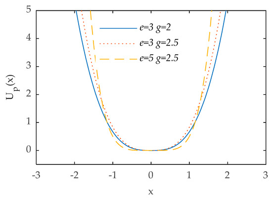
Figure 1.
Power function type single-well with different parameters.
2.1.2. Woods-Saxon Potential Model
The Woods-Saxon [37] is a nonlinear symmetric potential which can be expressed as follows:
where a forces the depth of potential, b affects the width of potential, and c dominates the steepness of the potential.
As shown in Figure 2, the shape of the Woods-Saxon potential function can be controlled by adjusting the values of the parameters (a, b, and c). From Figure 2, we can see that as the value of c increases, the steepness of the potential function becomes gentle, which indicates that the parameter c determines the wall steepness of the potential. Similarly, it can be seen that the depth of the potential has replaced, while the value of a is adjusted. We can notice that as b becomes larger, the width of the well also is increased. In summary, the effects of the parameters on the potential function in the Woods-Saxon are independent and has abundant potential function shapes.
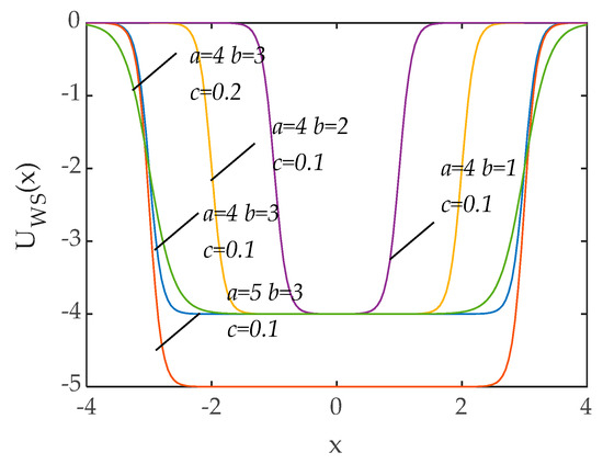
Figure 2.
Wood-Saxon potential with different parameters.
2.1.3. Joint Power Function and Woods-Saxon
We designed a new potential mode PWS which is a joint mode between the power function and Woods-Saxon. As is shown in Figure 3, and this new potential PWS can be expressed as:
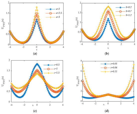
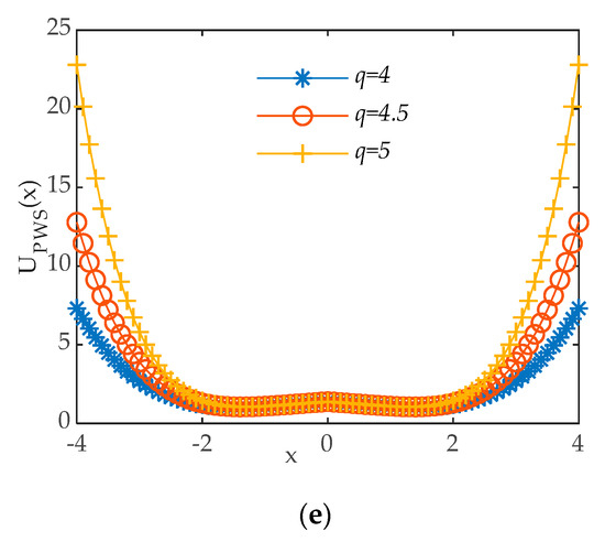
Figure 3.
(a) PWS b = 0.2, c = 0.5, e = 0.01, q = 4; (b) PWS a = 2, c = 0.5, e = 0.01, q = 4; (c) PWS a = 2, c = 1.2, e = 0.01, q = 4; (d) PWS a = 2, b = 1.2, c = 1.5, q = 4; € PWS a = 2, b = 1.2, c = 1.5, e = 0.11.
The novel potential function
contains five parameters a, b, c, g, e, and these parameters make PWS have flexible and variable potential function shapes, as shown in Figure 3.
In the SR system, noise, periodic signal, and potential function provide noise, periodic force, and potential well force, respectively. In general, the periodic force and the noise force are both fixed [42], so the realization of SR is largely determined by the nonlinear system that provides the potential well force provided by the potential function model. In this paper by adjusting the shapes of the potential function model to impose the SR phenomenon, the factors affecting the potential trap force include the steepness of the potential well wall and the height of the barrier. Because the potential well wall is too steep or too flat to achieve SR, or the barrier is too high or too low to achieve SR. Therefore, it is necessary to control the steepness of the potential well wall and the height of the barrier. Compared with the classical SR model, the potential function shape of the PWS model can have more changes by adjusting the parameters as shown in Figure 3, which means that the PWS model can better control the potential well force to achieve SR.
2.2. Stochastic Resonance
2.2.1. Classical Stochastic Resonance System
The SR phenomenon needs three basic conditions which are: (1) a nonlinear system, (2) a source of noise that is inherent in system or adds into the coherent input, and (3) weak coherent input signals [23]. The classical SR system can be described [38] as:
where A represents the weak periodic signal amplitude, and f0 is the weak periodic signal driving frequency, and n(t) is Gaussian white noise, which meets the following characteristics:
where D is noise intensity. denotes the reflection-symmetric quartic potential. It can be written as follows:
in which
a and b are real parameters. Substituting from (6) to (4), the classical function of SR can be described as:
2.2.2. PWS Stochastic Resonance System
We changed the traditional model into the new one—the PWS model. The new function of SR with PWS will be in the form:
where sgn(x) denotes the sign function. Moreover, it can be seen from Equation (8) that the system output depends on the input signal and the potential function model. Compared with Equation (4), the PWS SR system is different from the classical SR system only in the potential model. Besides, the SR system, input signal, and random noise simultaneously determine the SR phenomenon. In the actual situation, periodic force and the noise force are fixed. Therefore, the effectiveness of the SR system largely depends on the potential force, and a suitable potential model shape is an effective amplification of the weak fault signal guarantee.
2.3. Fourier Decomposition Method
The Fourier decomposition method (FDM) [40] is a new method of analyzing nonstationary signals. It is capable of expressing a multi-component signal x(t) with a sum of a particular set of consecutive single Fourier intrinsic band functions (FIBFs) and a residual component n(t), the model can be expressed as follows:
where FIBFs must meet the following constraints: (1) FIBFs are zero mean functions: ; (2) The FIBFs are orthogonal functions: ; (3) The FIBFs form the analytic FIBFs with instantaneous frequency and amplitude always greater than zero: with , , . According to the function of FDM, we use it to pre-process the input signals. First, the input signals will be decomposed into FIBFs using FDM. And then, we use the autocorrelation coefficient method to select potential FIBFs that have large correlation coefficients to reconstruct the signals and realize the pre-processing of the signals, it is because that the correlation coefficient reflects the tightness between FIBFs component and the original signals, in other words, with the increase of the correlation coefficient between FIBFs and original signals, the FIBFs will contain more information about bearings. Otherwise, there are two kinds of signal decomposition methods in FDM, i.e., from low frequency to high-frequency (LTH-FS) search and from high frequency to low-frequency (HTL-FS) search. It is important to note that the FDM decomposition method used in this paper is HTL-FS. In short, the proposed scheme for bearing fault diagnosis using PWS and FDM is summarized to have the key steps in Figure 4.
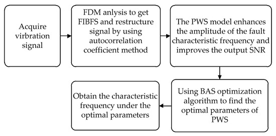
Figure 4.
The proposed scheme of bearing fault diagnosis with PWS and FDM.
3. Simulated Signal Analysis
To verify the superiority of the PWS and FDM (FDM-PWSR) method in enhancing the energy of weak signals, three-lamp test PWS, Classical SR, PWS, and FDM (FDM-CSR) are set up for comparison. Three sets of experiments were all adopted the frequency-shift and re-scaling method [26] to meet the small parameter requirements. We set the simulation signal S(t) for verification analysis, and S(t) settings as shown in Equation (11):
where A = 0.2, sampling frequency fs = 1024 Hz, and the sampling point number N is taken as 1024, the mixed-signal with noise intensity of D = 1 in time-domain, set fault frequency fa = 80 Hz and the coupled signals of the interference fe = 25 Hz. Figure 5a,b are the time domain waveform and frequency domain waveform of the simulated signal without noise, on the contrary, Figure 6a,b are the time domain waveform and frequency domain waveform of the simulated signal containing noise. Figure 7a,b are the time domain waveform and frequency domain waveform processed by classical SR, respectively. Similarly, Figure 8a,b are the time domain waveform and frequency domain waveform processed by PWS, respectively. It can be concluded from Figure 7b and Figure 8b that neither classical SR nor PWS are eliminating the coupled signals. The frequency of coupled signals fe and the frequency of bearings fault fa appear in the spectrogram simultaneously. It is hard to make sure which the frequency fe or fa is we needed. Under the influence of the coupled signals that may cause us to make a wrong judgment about the fault type of the faulty part. Otherwise, the frequency amplitude obtained after PWS processing is higher than that of classical SR, indicating that the ability of PWS to amplify the fault signal is stronger than the classical SR method.
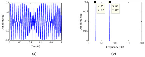
Figure 5.
(a) Time-domain waveform of the simulated signal without noise; (b) Frequency-domain waveform of the simulated signal without noise.
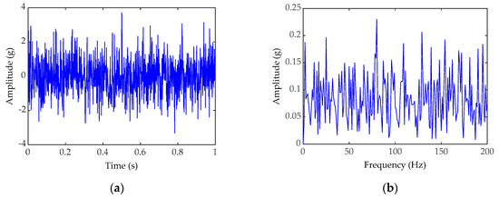
Figure 6.
(a) Time-domain waveform of the simulated signal with noise; (b) Frequency-domain waveform of the simulated signal containing noise.
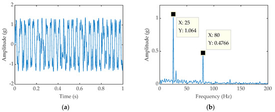
Figure 7.
(a) Time-domain waveform processed by classical SR; (b) Frequency-domain waveform processed by classical SR.
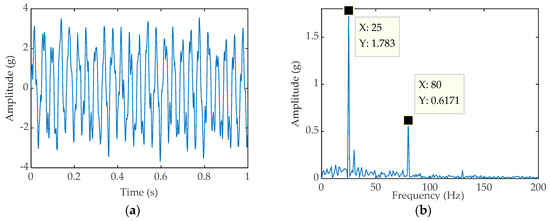
Figure 8.
(a) Time-domain waveform processed by PWS; (b) Frequency domain waveform processed by PWS.
Therefore, the classical SR and PWS are combined with the FDM method respectively. Figure 9a is the time domain diagram of FDM-CSR, Figure 9b is the spectrum diagram of FDM-CSR. Figure 10a is the time domain diagram of FDM-PWSR, and Figure 10b is the spectrum diagram of FDM-PWSR.
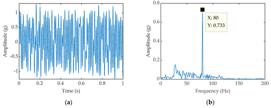
Figure 9.
(a) Time-domain waveform processed by classical FDM-CSR; (b) Frequency domain waveform processed by FDM-CSR, a = 0.1, b = 1.
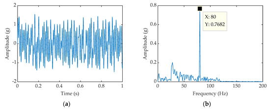
Figure 10.
(a) Time-domain waveform processed by FDM-PWSR; (b) Frequency domain waveform processed by FDM-PWSR, a = 5, b = 17.2, c = 40.79, e = 0.073, g = 4.
As shown in Figure 9b and Figure 10b, the peak value of the spectrogram of FDM-CSR is 0.733 mv, and the peak value of the spectrogram of FDM-PWSR is 0.7682 mv. At the same time, the SNR of FDM-CSR is calculated as −11.69, the SNR of FDM-PWSR is −11.14. So we can see that the signal processing effect of FDM-PWSR is better than that of FDM-CSR.
In other words, PWS performs better to amplify the fault signal is stronger compared with the traditional SR method. Further, FDM is used to reduce the influence of coupled signals, also the amplitude and SNR of the signals obtained by PWS is better than classical SR. The results show that the PWS method is better than the classical SR method in enhancing the weak signal energy and the combination of PWS and FDM can further improve the weak signal energy detected.
4. Experimental Verification
To verify the feasibility of the method in this paper, we collected vibration signals of the bearings in a wind turbine. The bearing vibration signals come from the input shaft of the wind turbine gearbox. The current rotational speed of the bearing is 10 rpm. It is worth mentioning that the signals come from a healthy wind turbine. The input shaft vibration signal mainly includes the spindle’s rotation signal, other coupling information, and noise interference in the environment. The signal was acquired at a sample rate of 10.24 kHz. The signal length is of 4 s. The original signals’ time-domain diagram is shown in Figure 11a, from which we can see that there is serious interference in the signal, and the main shaft rotation period cannot be identified, the rotation frequency else cannot be observed from the frequency domain diagram shown in Figure 11b. The original signal is input into the PWS system to obtain the time domain diagram (shown in Figure 12a) and the frequency domain diagram (shown in Figure 12b). At the same time, the frequency with the largest amplitude is observed to be 0.25 Hz from the diagram of Figure 12b, which is much larger than the actual bearing rotation frequency of 0.167 Hz; similarly, the original signals inputted into classic SR system to obtain the time domain diagram (shown in Figure 13a) and the frequency domain diagram (shown in Figure 13b). From the picture of Figure 13b, the most significant frequency is 0.25 Hz, which is also inconsistent with the actual frequency value to be detected, although the SR has the function of signal energy enhancement, it cannot eliminate the interference of the coupling signal, which limits the weak signal detection capability of SR. It is can be seen that the original signals are reconstructed by the FDM and the reconstructed signal time-domain diagram (shown in Figure 14).
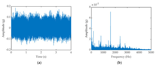
Figure 11.
(a) Time-domain waveform of original signals; (b) The vibration signal frequency-domain waveform of original signals.
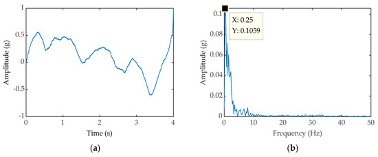
Figure 12.
(a) Time-domain waveform processed by PWS; (b) Frequency-domain waveform processed by PWS.
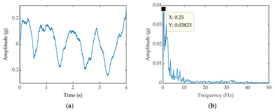
Figure 13.
(a) Time-domain waveform processed by classical SR; (b) Frequency-domain waveform processed by classical SR.
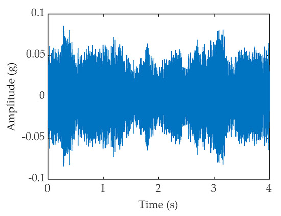
Figure 14.
Time-domain waveform of the reconstructed signal.
Thus, we use FDM to preprocess the vibration signals and the specific steps are as shown in the flow chart as shown in Figure 4. The reconstructed signals are inputted into the PWS system. We can obtain the time domain diagram (shown in Figure 15a) and frequency domain diagram (shown in Figure 15b), we learn that the amplitude of characteristics frequency is 0.2957 mV. The SNR is equal to −0.1127 dB. Simultaneously we take the reconstructed signals into the conventional SR system, the time domain diagram (shown in Figure 16a), and the frequency domain diagram (shown in Figure 16b) can be obtained, and the amplitude of characteristics frequency is 0.2226 mV. The SNR is equal to −0.1407 dB.
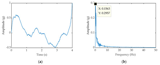
Figure 15.
(a) Time-domain waveform processed by FDM-PWSR; (b) Frequency-domain waveform processed by FDM-PWSR.
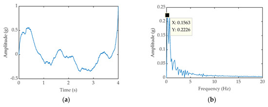
Figure 16.
(a) Time-domain waveform processed by FDM-CSR; (b) Frequency-domain waveform processed by FDM-CSR.
Comparing Figure 15b and Figure 16b, it can be seen that both the methods of FDM-CSR have detected the frequency of 0.1563 Hz, which are very close to the theoretical value of the bearing rotational frequency 0.1667 Hz. The reason for the slight error is that the original signals are subject to complex interference in the actual situation. Further, the amplitude of characteristics frequency in Figure 15b is larger than that in Figure 16b. This is to indicate that the PWS is better than the traditional SR system in boosting weak signals energy.
All of the above proves that the PWS system is superior to the traditional SR system about enhancing weak signals energy. The FDM method can effectively reduce the influence of coupled signals to improve the accuracy of the SR method in detecting and extracting weak signals.
Further, we analyzed a set of published vibration data [43] of the output shaft bearing of the wind turbine. The known sampling frequency is 12.8 kHz, the sampling time is 1.28 s, the bearing rolls off, the reference value of the fault frequency is 0.7813 Hz, FDM-PWSR processing Time domain and frequency domain graphs obtained in the future (Figure 17a,b), SNR = −0.6649 dB, time-domain graph and frequency domain graph obtained by FDM-CSR method (Figure 18a,b), SNR = −1.2881 dB.
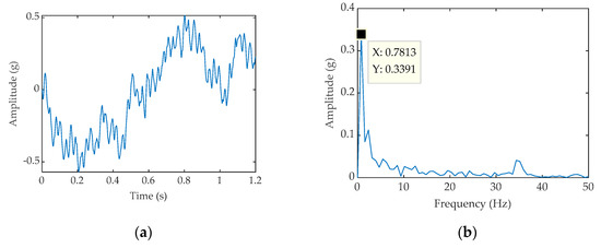
Figure 17.
(a) Time-domain waveform processed by FDM-PWSR; (b) Frequency-domain waveform processed by FDM-PWSR.
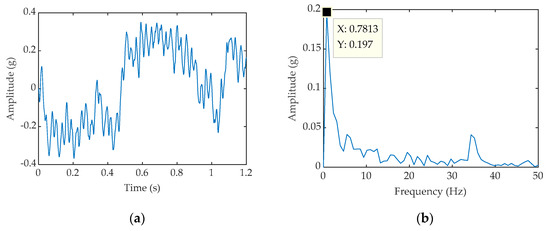
Figure 18.
(a) Time-domain waveform processed by FDM-CSR; (b) Frequency-domain waveform processed by FDM-CSR.
5. Conclusions
A new potential function PWS is proposed for strengthening the energy of weak signals, which has an extremely rich potential function shapes to match different signal requirements. From the simulation and experimental results, it can be seen that PWS can obtain higher SNR and larger characteristics frequency amplitude than classical SR, which proves that PWS is superior to classical SR. At the same time, FDM can solve the coupled issue in complex signals, which can improve the accuracy of PWS extracting weak signals, so we combine the PWS and FDM methods to further improve the detection accuracy. From the experimental analysis, we can conclude that the method proposed in this paper can achieve effects that FDM, PWS, and SR can’t have. Under the same conditions, that is, the input signal is pre-processed by FDM, and the signal obtained by the PWS method is better than the result gained by the classical SR from the amplitude and SNR, which proves the effectiveness of the proposed method.
Author Contributions
Formal analysis, B.F.; Investigation, Y.X.; Project administration, J.W.; Software, B.Z.; Supervision, F.G.; Writing—original draft, C.Z.; Writing—review & editing, H.D. All authors have read and agreed to the published version of the manuscript.
Funding
This research was funded by The National Natural Science Foundation of China, grant number: 51965052; 51565046.
Acknowledgments
The authors would like to thank Beijing Tianrun New Energy Investment Co., Ltd. and Luleå University of Technology for providing a large amount of experimental data, and Inner Mongolia Key Laboratory of Intelligent Diagnosis and Control of Mechatronic Systems for excellent technical support.
Conflicts of Interest
The authors declare no conflict of interest.
References
- Wang, J.; Qiao, W.; Qu, L. Wind Turbine Bearing Fault Diagnosis Based on Sparse Representation of Condition Monitoring Signals. IEEE Trans. Ind. Appl. 2019, 55, 1844–1852. [Google Scholar] [CrossRef]
- Koukoura, S.; Carroll, J.; Weiss, S.; McDonald, A. Wind turbine gearbox vibration signal signature and fault development through time. In Proceedings of the 2017 25th European Signal Processing Conference (EUSIPCO), Kos Island, Greece, 28 August–2 September 2017; pp. 1380–1384. [Google Scholar]
- Barbini, L.; Cole, M.O.; Hillis, A.; Du Bois, J.L. Weak signal detection based on two dimensional stochastic resonance. In Proceedings of the 23rd European Signal Processing Conference (EUSIPCO), Nice, France, 31 August–4 September 2015; Institute of Electrical and Electronics Engineers (IEEE): Piscataway, NJ, USA, 2015; pp. 2147–2151. [Google Scholar]
- Yang, C.; Jia, M. A novel weak fault signal detection approach for a rolling bearing using variational mode decomposition and phase space parallel factor analysis. Meas. Sci. Technol. 2019, 30, 115004. [Google Scholar] [CrossRef]
- Lu, S.; Zheng, P.; Liu, Y.; Cao, Z.; Yang, H.; Wang, Q. Sound-aided vibration weak signal enhancement for bearing fault detection by using adaptive stochastic resonance. J. Sound Vib. 2019, 449, 18–29. [Google Scholar] [CrossRef]
- Wang, J.; Xu, M.; Zhang, C.; Huang, B.; Gu, F. Online Bearing Clearance Monitoring Based on an Accurate Vibration Analysis. Energies 2020, 13, 389. [Google Scholar] [CrossRef]
- Fan, Y.; Zhang, C.; Xue, Y.; Wang, J.; Gu, F. A Bearing Fault Diagnosis Using a Support Vector Machine Optimised by the Self-Regulating Particle Swarm. Shock. Vib. 2020, 2020, 9096852. [Google Scholar] [CrossRef]
- Huang, N.E.; Shen, Z.; Long, S.R.; Wu, M.C.; Shih, H.H.; Zheng, Q.; Yen, N.-C.; Tung, C.C.; Liu, H.H. The empirical mode decomposition and the Hilbert spectrum for nonlinear and non-stationary time series analysis. Proc. R. Soc. A Math. Phys. Eng. Sci. 1998, 454, 903–995. [Google Scholar] [CrossRef]
- Wu, Z.; Huang, N.E. A study of the characteristics of white noise using the empirical mode decomposition method. Proc. R. Soc. A: Math. Phys. Eng. Sci. 2004, 460, 1597–1611. [Google Scholar] [CrossRef]
- Wu, Z.; Huang, N.E. Ensemble empirical mode decomposition: a noise-assisted data analysis method. Adv. Adapt. Data Anal. 2009, 1, 1–41. [Google Scholar] [CrossRef]
- McDonald, G.L.; Zhao, Q.; Zuo, M.J. Maximum correlated Kurtosis deconvolution and application on gear tooth chip fault detection. Mech. Syst. Signal. Process. 2012, 33, 237–255. [Google Scholar] [CrossRef]
- Dubey, G.; Dwivedi, R. Rolling Element Bearing Fault Detection Through Adaptive Filtering Wavelet Transform Using Vibration & Current Signals. Int. J. Curr. Eng. Sci. Res. 2016, 3, 22–26. [Google Scholar]
- Liu, F.; Yang, L.; Shi, R. Weak Life Signal Detection Based on Wavelet Transform and Threshold De-noising Theory. Rev. Tec. Fac. Ing. Univ. Zulia 2016, 39, 54–60. [Google Scholar] [CrossRef]
- He, L.-F.; Cao, L.; Zhang, G.; Yi, T. Weak signal detection based on underdamped stochastic resonance with an exponential bistable potential. Chin. J. Phys. 2018, 56, 1588–1598. [Google Scholar] [CrossRef]
- Benzi, R.; Parisi, G.; Sutera, A.; Vulpiani, A. A Theory of Stochastic Resonance in Climatic Change. SIAM J. Appl. Math. 1983, 43, 565–578. [Google Scholar] [CrossRef]
- Benzi, R.; Parisi, G.; Sutera, A.; Vulpiani, A. Stochastic resonance in climate change. Tellus 2010, 34, 10–16. [Google Scholar]
- Kojima, N.; Lamsal, B.; Matsumoto, N.; Yamashiro, M. Proposing autotuning image enhancement method using stochastic resonance. Electron. Commun. Jpn. 2019, 102, 1–12. [Google Scholar] [CrossRef]
- Niu, S.-Y.; Guo, L.-Z.; Li, Y. Boundary-Preserved Deep Denoising of the Stochastic Resonance Enhanced Multiphoton Images. arXiv 2019, arXiv:1904.06329. [Google Scholar]
- Gu, X.; Chen, C. Adaptive parameter-matching method of SR algorithm for fault diagnosis of wind turbine bearing. J. Mech. Sci. Technol. 2019, 33, 1007–1018. [Google Scholar] [CrossRef]
- Zhang, J.; Yang, J.-H.; Litak, G.; Hu, E. Feature extraction under bounded noise background and its application in low speed bearing fault diagnosis. J. Mech. Sci. Technol. 2019, 33, 3193–3204. [Google Scholar] [CrossRef]
- Chi, K.; Kang, J.; Zhang, X.; Zhao, F. Effect of scale-varying fractional-order stochastic resonance by simulation and its application in bearing diagnosis. Int. J. Model. Simul. Sci. Comput. 2019, 10, 1–21. [Google Scholar] [CrossRef]
- He, D.; Chen, X.; Pei, L.; Jiang, L.; Yu, W. Improvement of Noise Uncertainty and Signal-To-Noise Ratio Wall in Spectrum Sensing Based on Optimal Stochastic Resonance. Sensors 2019, 19, 841. [Google Scholar] [CrossRef]
- Tadokoro, Y.; Tanaka, H.; Nakashima, Y.; Yamazato, T.; Arai, S. Enhancing a BPSK receiver by employing a practical parallel network with Stochastic resonance. Nonlinear Theory Appl. IEICE 2019, 10, 106–114. [Google Scholar] [CrossRef]
- Jiang, X.; Diao, M.; Qu, S. Signal Detection Algorithm Design Based on Stochastic Resonance Technology Under Low Signal-to-Noise Ratio. J. Shanghai Jiaotong Univ. 2019, 24, 328–334. [Google Scholar] [CrossRef]
- Yao, Y.; Yang, L.; Wang, C.; Liu, Q.; Gui, R.; Xiong, J.; Yi, M. Subthreshold Periodic Signal Detection by Bounded Noise-Induced Resonance in the FitzHugh–Nagumo Neuron. Complexity 2018, 2018, 5632650. [Google Scholar] [CrossRef]
- Fan, S.; Wang, T.; Leng, Y.; Wang, W. Detection of Weak Periodic Impact Signals Based on Scale Transformation Stochastic Resonance. China Mech. Eng. 2006, 17, 387–390. [Google Scholar]
- Tan, J.; Chen, X.; Wang, J.; Chen, H.; Cao, H.; Zi, Y.; He, Z. Study of frequency-shifted and re-scaling stochastic resonance and its application to fault diagnosis. Mech. Syst. Signal. Process. 2009, 23, 811–822. [Google Scholar] [CrossRef]
- Kumar, S.; Jha, R.K. Noise-Induced Resonance and Particle Swarm Optimization-Based Weak Signal Detection. Circuits Syst. Signal. Process. 2018, 38, 2677–2702. [Google Scholar] [CrossRef]
- He, L.; Hu, D.; Zhang, G.; Lu, S. Stochastic resonance in asymmetric time-delayed bistable system under multiplicative and additive noise and its applications in bearing fault detection. Mod. Phys. Lett. B 2019, 33, 1950341. [Google Scholar] [CrossRef]
- Hu, B.; Guo, C.; Wu, J.; Tang, J.; Zhang, J.; Wang, Y. An Adaptive Periodical Stochastic Resonance Method Based on the Grey Wolf Optimizer Algorithm and Its Application in Rolling Bearing Fault Diagnosis. J. Vib. Acoust. 2019, 141, 041016-30. [Google Scholar] [CrossRef]
- Tang, J.; Shi, B.; Li, Z. Asymmetric delay feedback stochastic resonance detection method based on prior knowledge particle swarm optimization. Chin. J. Phys. 2018, 56, 2104–2118. [Google Scholar] [CrossRef]
- Zhe, J.; Li, G.; Zhang, R. Stochastic Resonance Based on Quantum Genetic Algorithm and Applications in Weak Signal Detection; Atlantis Press: Shenyang, China, 2015; pp. 2120–2124. [Google Scholar]
- YuanDong, J.; Lu, Z.; MaoKang, L. Generalized stochastic resonance of power function type single-well system. Acta Phys. Sin. 2014, 63, 242–252. [Google Scholar]
- Tang, R. A New Second-Order Bistable Adaptive Stochastic Resonance Noise Reduction Method; Atlantis Press: Shenyang, China, 2018; pp. 121–125. [Google Scholar]
- Chen, Z.; Ning, L.J. Impact of depth and location of the wells on vibrational resonance in a triple-well system. Pramana 2018, 90, 49. [Google Scholar] [CrossRef]
- Liu, Y.; Wang, F.; Liu, L.; Zhu, Y. Symmetry tristable stochastic resonance induced by parameter under levy noise background. Eur. Phys. J. B 2019, 92, 161–168. [Google Scholar] [CrossRef]
- Lu, L.; Yuan, Y.; Wang, H.; Zhao, X.; Zheng, J. A New Second-Order Tristable Stochastic Resonance Method for Fault Diagnosis. Symmetry 2019, 11, 965. [Google Scholar] [CrossRef]
- Jialei, D. Study on incipient fault diagnosis of machinery based on piecewise linearity and unsaturated stochastic resonance. China Meas. Test. Technol. 2017, 43, 106–112. [Google Scholar]
- Woods, R.D.; Saxon, D.S. Diffuse Surface Optical Model for Nucleon-Nuclei Scattering. Phys. Rev. 1954, 95, 577–578. [Google Scholar] [CrossRef]
- Singh, P.; Joshi, S.D.; Patney, R.K.; Saha, K. The Fourier decomposition method for nonlinear and non-stationary time series analysis. Proc. R. Soc. A Math. Phys. Eng. Sci. 2017, 473, 20160871. [Google Scholar] [CrossRef]
- Jiang, X.; Li, S. BAS: Beetle Antennae Search Algorithm for Optimization Problems. Int. J. Robot. Control. 2018, 1, 1. [Google Scholar] [CrossRef]
- Li, H. Weak Fault Enhancement Method for Blade Crack by Using Stochastic Resonance. Chin. J. Mech. Eng. 2016, 52, 94–101. [Google Scholar] [CrossRef]
- Strömbergsson, D.; Marklund, P.; Berglund, K.; Larsson, P. Bearing monitoring in the wind turbine drivetrain: A comparative study of the FFT and wavelet transforms. Wind. Energy 2020, 23, 1381–1393. [Google Scholar] [CrossRef]


Publisher’s Note: MDPI stays neutral with regard to jurisdictional claims in published maps and institutional affiliations. |
© 2020 by the authors. Licensee MDPI, Basel, Switzerland. This article is an open access article distributed under the terms and conditions of the Creative Commons Attribution (CC BY) license (http://creativecommons.org/licenses/by/4.0/).