Control Techniques for a Single-Phase Matrix Converter

Abstract

The single-phase matrix converter is an AC-AC power topology which consists of six bidirectional switches and it is considered the key unit in cascade or multilevel configurations. In this paper, a comparison between two control techniques is presented, one based on a proportional-integral-derivative control module with a pulse width modulator, and the other known as finite-state model predictive control. Simulation and experimental results are presented and discussed to demonstrate the feasibility and performance of both techniques.

1. Introduction

The definition of the matrix converter was released in the technical literature in 1976 by Gyugi and Pelly [1]. At that time, it was considered as a revolutionary topology due to the combination of switches without energy storage elements which can be used to generate output voltages with arbitrary amplitude and frequency. Then more extensive research was presented by Venturini and Alesina in the 1980s [2,3], giving a more robust definition of this converter.

A direct matrix converter (DMC) comprises a number of bidirectional semiconductors arranged in a matrix structure to perform direct AC-AC conversion. Unlike classical AC-DC-AC conversion, the DMC does not require a storage DC-link element and constitutes a single-stage power conversion system. The absence of a storage element improves efficiency, reduces volume, increases service life, and reduces the complexity of control schemes [4]. Only small filters are considered to eliminate the harmonic distortion produced by the commutation of the switches. The main advantages of matrix converters which make them attractive are sinusoidal input and output waveforms, possibility to work a unity power factor, compact nature, and bidirectional power flow.

Many modulation and control strategies have been proposed for matrix converters [5]. Generally, modulation strategies can be classified into (1) scalar techniques (e.g., the Venturini method [6]), (2) PWM methods (carrier- and SVM-based) [7], and (3) other control strategies (such as hysteresis current control [8], predictive control [9], sliding mode control (SMC) [10], direct torque control (DTC) [11], diffuse method [12], neural networks [13], active damping control [14], and PR controller [15]).

In terms of applications, this matrix converter configuration mainly encompasses solutions aimed at a decrease in volume and weight, which results in high energy density considering that the converter does not require energy storage elements to achieve good performance.

Because of these characteristics, companies like Yaskawa have intensified their offer of matrix converters in formal trading [16]. Some interesting examples of applications at the industrial level are (1) radio frequency induction heating, because it needs a high-frequency AC power supply (usually 100 to 200 kHz) and classical AC-DC-AC topologies that use bulky storage components that require complex algorithms to allow unit power factor means that this topology becomes attractive [17]; (2) wireless power transfer systems (WPT) implement unreliable and bulky DC link capacitors, a problem that is solved by employing a single-phase matrix converter (SPMC) to transform power from low-frequency networks to high-power coils in vehicle-to-grid (V2G) applications [18]; and (3) energy saving by feeding street lights comparing the use of the SPMC on the conventional autotransformer, increasing efficiency by 15% [19].

The main contribution of this paper is the experimental comparison between two simple control strategies to track the output current of a SPMC, a Sinusoidal Pulse Width Modulation (SPWM) technique with a PI linear controller, and a Finite States Model Predictive Control (FS-MPC) strategy. The comparative study is done in terms of harmonic distortion, dynamic response and steady state. Section 2 introduces the SPMC topology, and then Section 3 and Section 4 describe the two controllers. Finally, the behavior of both controllers is demonstrated in Section 4.

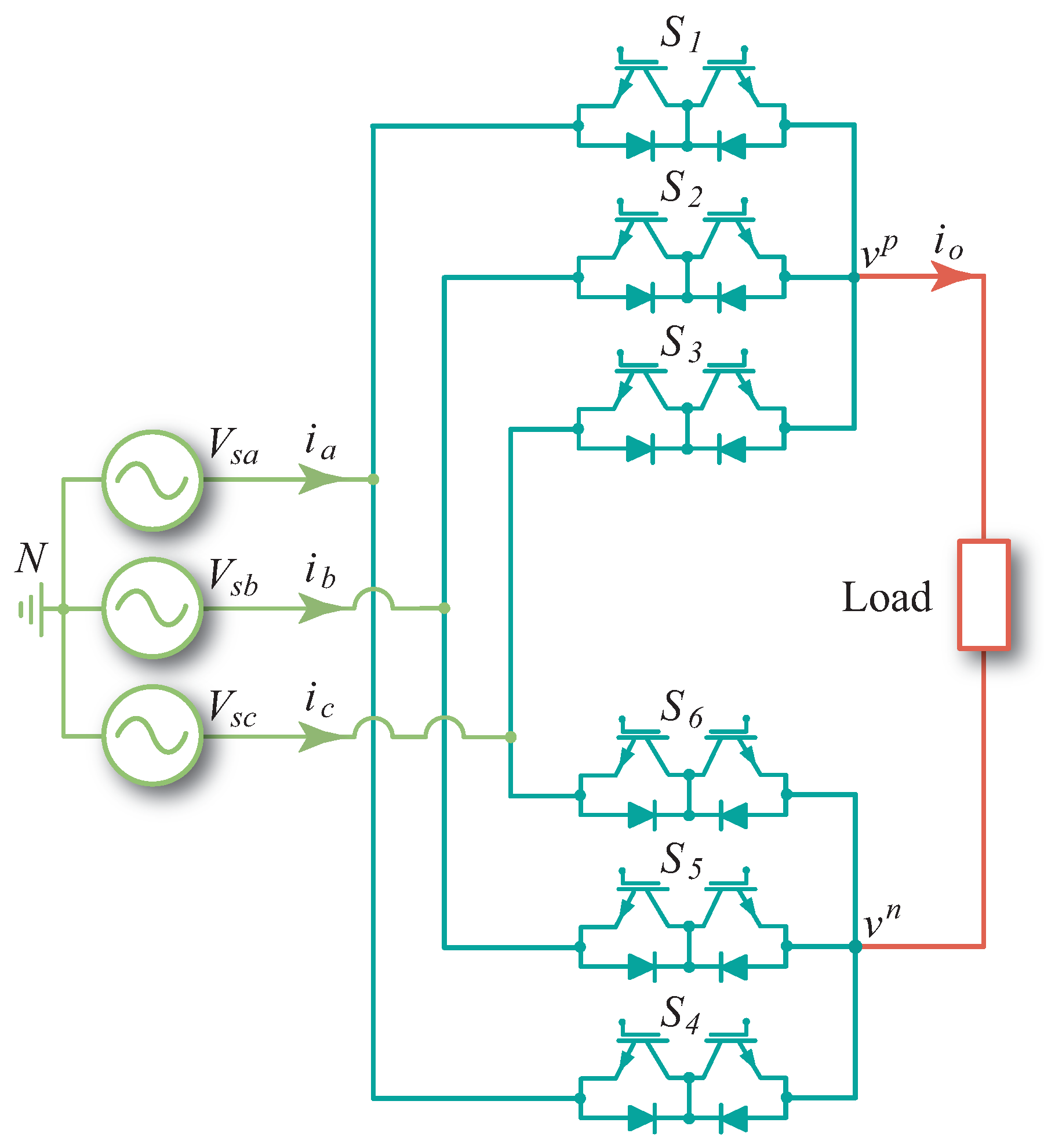
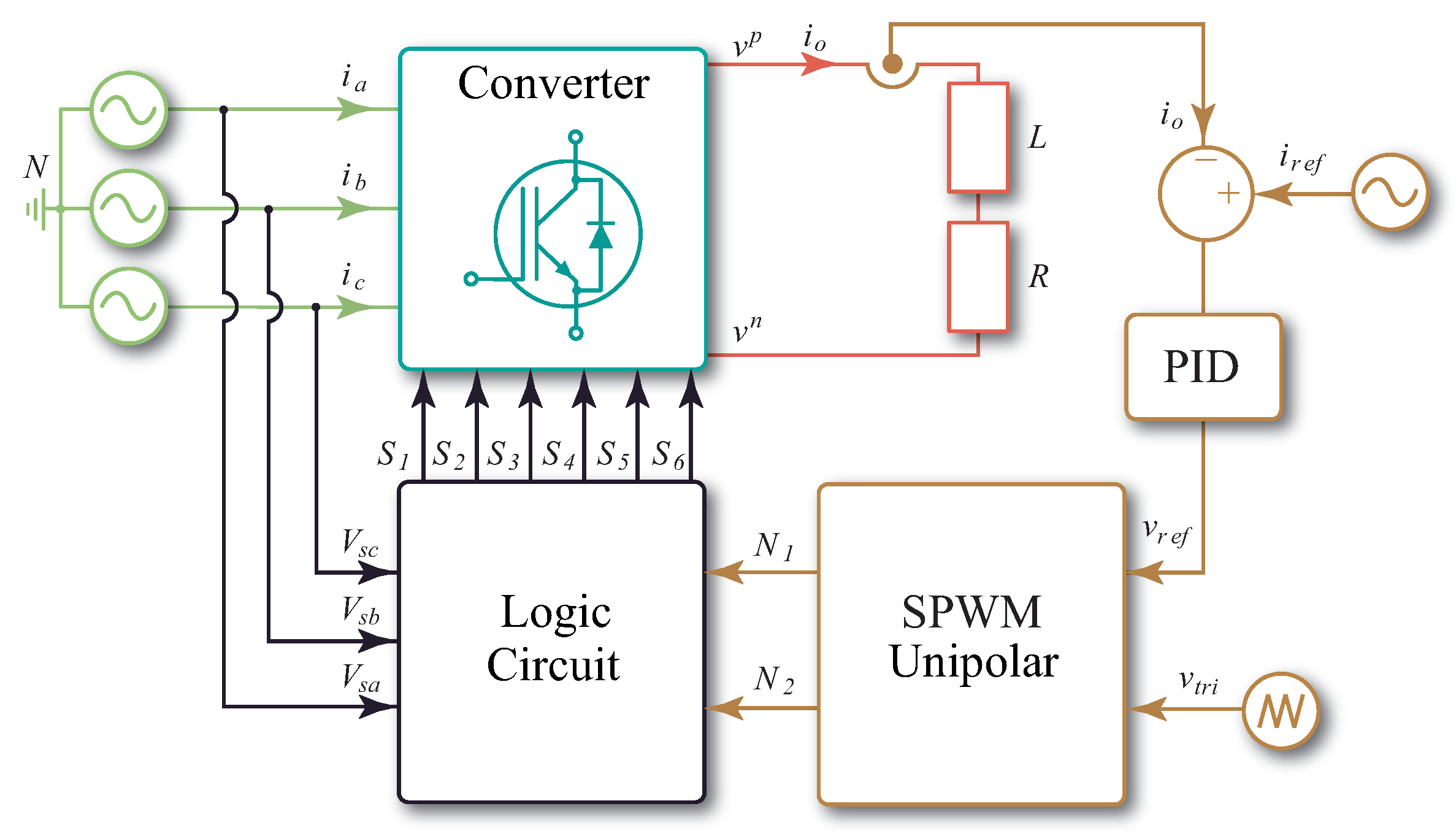
2. Single-Phase Matrix Converter 3 × 2 (SPMC)

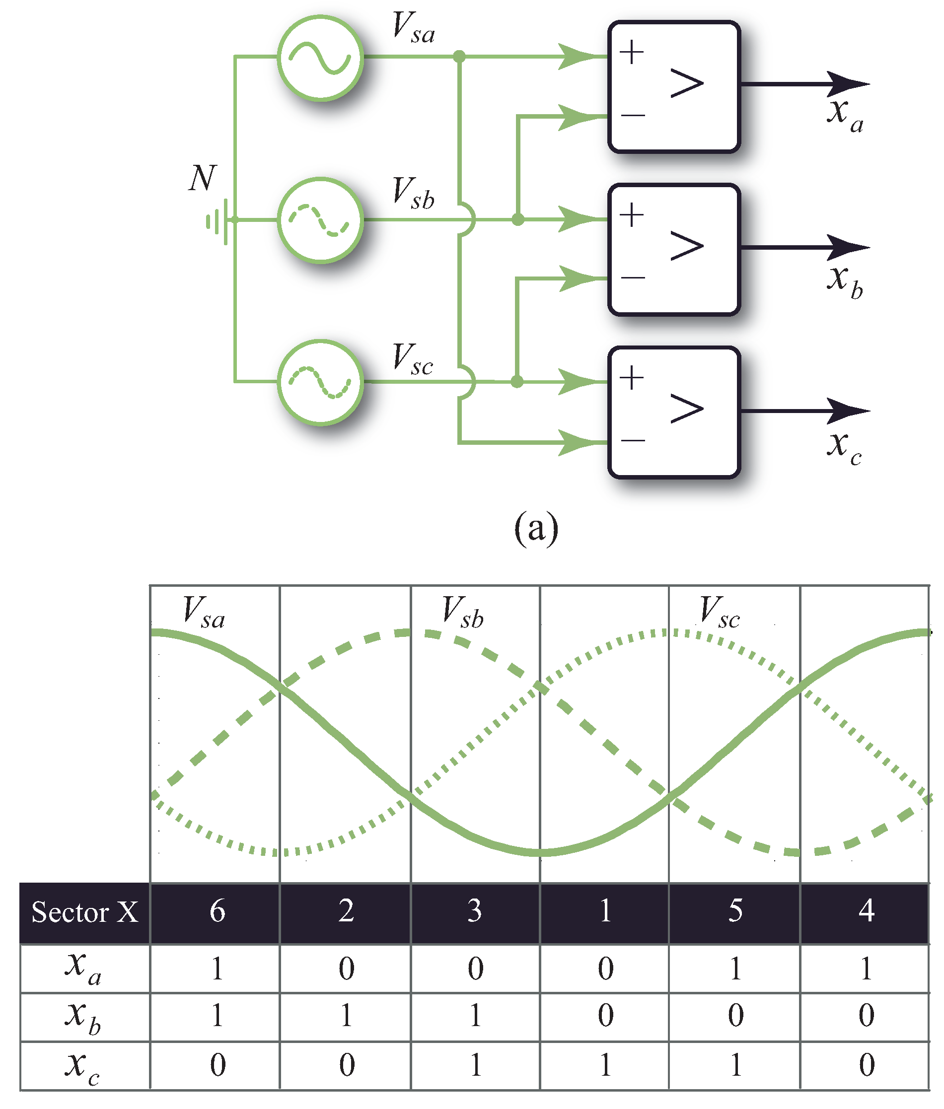
The power topology of the 3 × 2 SPMC is presented in Figure 1. This type of converter is called a direct converter because it only has one conversion stage and consists of six bidirectional switches where $S_1$, $S_2$, and $S_3$ are for the phase line and $S_4$, $S_5$, and $S_6$ are for the neutral line. By concatenating the state of the six bidirectional switches into a single vector, it is possible to obtain the mathematical model of the converter. In this way, the output voltage $v=\left[v^p-v^n\right]$ depends directly on the input voltages $(V_{sa},V_{sb}$ and $V_{sc})$ and the current state of the switches $(S_1$ to $S_6)$ listed in

Table 1. Space vector of single-phase matrix converter shown in Figure 1.

j	Output		Trigger Pulses
$\mathit{j}$	${\mathit{v}}^{\mathit{p}}$	${\mathit{v}}^{\mathit{n}}$	$S_1$	$S_2$	$S_3$	$S_4$	$S_5$	$S_6$
1	$V_{sa}$	$V_{sa}$	1	0	0	1	0	0
2	$V_{sa}$	$V_{sb}$	1	0	0	0	1	0
3	$V_{sa}$	$V_{sc}$	1	0	0	0	0	1
4	$V_{sb}$	$V_{sa}$	0	1	0	1	0	0
5	$V_{sb}$	$V_{sb}$	0	1	0	0	1	0
6	$V_{sb}$	$V_{sc}$	0	1	0	0	0	1
7	$V_{sc}$	$V_{sa}$	0	0	1	1	0	0
8	$V_{sc}$	$V_{sb}$	0	0	1	0	1	0
9	$V_{sc}$	$V_{sc}$	0	0	1	0	0	1

.

3. SPWM with Classic Linear Controller

In order to digitally control the switching commutation in a power converter, a classic Pulse Width Modulation (PWM) technique is used [20]. Originally, this technique was used in inverters; however, due to its simplicity, it has been implemented in various topologies of power converters, and it is now widely used on an industrial application. This type of modulation has a variety of advantages such as reduction of filtering requirements, low amount of mathematical calculations, and increase in the transmission of effective power.

The proposed control strategy consists of (1) a modulation responsible for delivering the voltage levels that the converter must generate, (2) a logic circuit that is dedicated to sectoring the input voltages, and finally (3) a proportional-integral-derivative (PID) controller for closed loop control of the load current [21].

The modulation scheme consists of two fundamental parts: The first is responsible for performing the SPWM scheme with which a modulated signal equivalent to the reference sinusoidal wave is generated. A second part is dedicated to sectoring the three-phase input source in order to identify the different voltage zones, given by the different line-line voltage combinations. It is important to mention that while the PID controller is primarily used in processes that offer linear responses, it can be used for rotational variables when considering that the speed at which the control algorithm is executed is very high in comparison to the variation in the time of the reference. It can be said that the horizon under which the controller is executed is therefore linear.

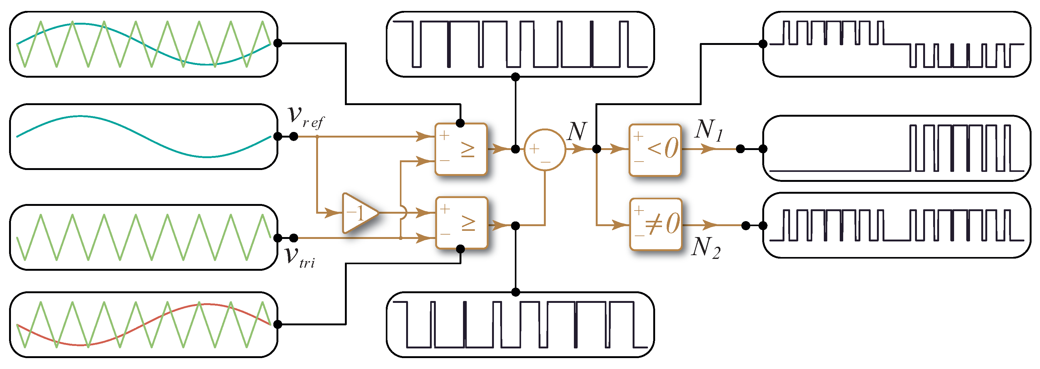
3.1. Unipolar SPWM Modulation

Sinusoidal Pulse Width Modulation (SPWM) basically consists of generating pulses of width proportional to the amplitude of a modulating or reference signal $\left(v_{ref}\right)$, which consists of a typical sinusoidal signal that is compared with a carrier signal $\left(v_{tri}\right)$, whose shape is triangular. The intersection points delineate the times when the rising and lowering flanks of variable width pulses occur, thus generating a resulting signal that implicitly includes all the information about the modulating wave (amplitude and frequency) where the end is to be able to transmit these features to the power side, reproducing the pulses with the action of the commutation devices. The diagram of this kind of modulation is shown in Figure 2. In addition to appreciating the blocks corresponding to the unipolar SPWM two blocks coupled to the output (N) are shown. These comparator blocks fulfill the function of transforming the three voltage levels into binary signals. Figure 2 also shows the result of comparisons between sinusoidal and triangular signals in both comparators. Finally, in this figure is clearly that the pulsating output signal N is composed of three levels and implicitly contains the frequency of the modulating signal.

3.2. Three-Phase AC Source Sectorization

For a three-phase sinusoidal input source, the identification of the different voltage zones is of great importance for the choice of devices to be commutated. In Figure 3b, the sectoring of the input source is depicted in terms of the voltages values supplied over time. These different sectors are framed under the variables $x_a$, $x_b$, and $x_c$, signals that are generated by using binary comparators, which determine whether the phase stress is greater than the following (as shown in Figure 3a). Finally, by means of the information provided by the modulator about the voltage levels generated $(N_1,N_0)$ and the information provided by the comparator blocks that get the sector of the three-phase input source $(x_a$, $x_b$, and $x_c)$ and by using

Table 2. Space vector of a single phase matrix converter shown in Figure 1 by the PID+SPWM scheme with AC source sectorization.

	${\mathit{N}}_2$	${\mathit{N}}_1$	X	Output		Trigger Pulses
				${\mathit{v}}^{\mathit{p}}$	${\mathit{v}}^{\mathit{n}}$	${\mathit{S}}_{\mathbf{1}}$	${\mathit{S}}_{\mathbf{2}}$	${\mathit{S}}_{\mathbf{3}}$	${\mathit{S}}_{\mathbf{4}}$	${\mathit{S}}_{\mathbf{5}}$	${\mathit{S}}_{\mathbf{6}}$
1	0	1	6	$V_{sa}$	$V_{sc}$	1	0	0	0	0	1
2	0	1	2	$V_{sb}$	$V_{sc}$	0	1	0	0	0	1
3	0	1	3	$V_{sb}$	$V_{sa}$	0	1	0	1	0	0
4	0	1	1	$V_{sc}$	$V_{sa}$	0	0	1	1	0	0
5	0	1	5	$V_{sc}$	$V_{sb}$	0	0	1	0	1	0
6	0	1	4	$V_{sa}$	$V_{sb}$	1	0	0	0	1	0
7	1	1	6	$V_{sc}$	$V_{sa}$	0	0	1	1	0	0
8	1	1	2	$V_{sc}$	$V_{sb}$	0	0	1	0	1	0
9	1	1	3	$V_{sa}$	$V_{sb}$	1	0	0	0	1	0
10	1	1	1	$V_{sa}$	$V_{sc}$	1	0	0	0	0	1
11	1	1	5	$V_{sb}$	$V_{sc}$	0	1	0	0	0	1
12	1	1	4	$V_{sb}$	$V_{sa}$	0	1	0	1	0	0
13	0	0	6	$V_{sc}$	$V_{sc}$	0	0	1	0	0	1
14	0	0	2	$V_{sc}$	$V_{sc}$	0	0	1	0	0	1
15	0	0	3	$V_{sa}$	$V_{sa}$	1	0	0	1	0	0
16	0	0	1	$V_{sa}$	$V_{sa}$	1	0	0	1	0	0
17	0	0	5	$V_{sb}$	$V_{sb}$	0	1	0	0	1	0
18	0	0	4	$V_{sb}$	$V_{sb}$	0	1	0	0	1	0

, the switching signals for the SPMC are obtained.

The process described in the previous paragraphs make up the integrated scheme of control PID+SPWM (Figure 4).

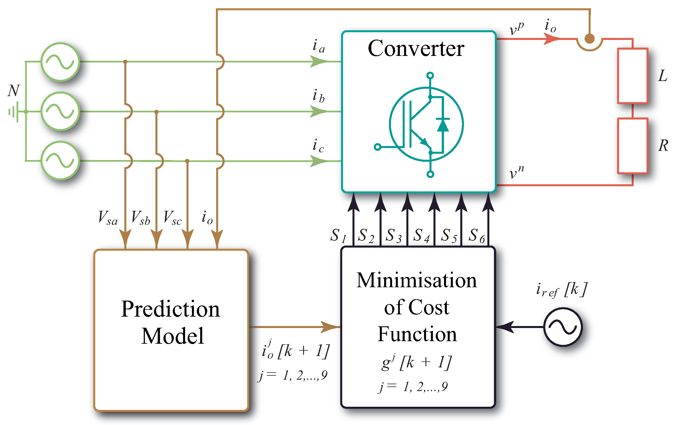
4. Predictive Controller for the SPMC

Model-based Predictive Control (MPC) [22,23] is placed within what are called optimal controllers. That is, those in which control is handled around the optimization of a criterion that is directly linked to the future behavior of the system. Its main advantages are the ease of implementation, rapid dynamic response, and operation under multivariable models. Logically, this control also has certain drawbacks mainly linked to its implementation. One of them is that the quality of the controller is directly connected to an adequate mathematical model of the system. Thus, a more accurate model would lead to less error and therefore better behavior in a steady state. However, external variables such as temperature and electromagnetic effects have influence in the electrical system generating changes in its mathematical model.

MPC is a methodology for calculating control actions. This considers that the controller knows the behavior of the system (model) and may therefore be able to correctly predict its dynamic evolution. Consequently, it can evaluate the different combinations of control actions over a time horizon depending on the degree of compliance with them (cost function). Then, with this knowledge the controller is able to find the most optimal solution that maximizes the performance of the variable to be controlled.

4.1. Prediction Model

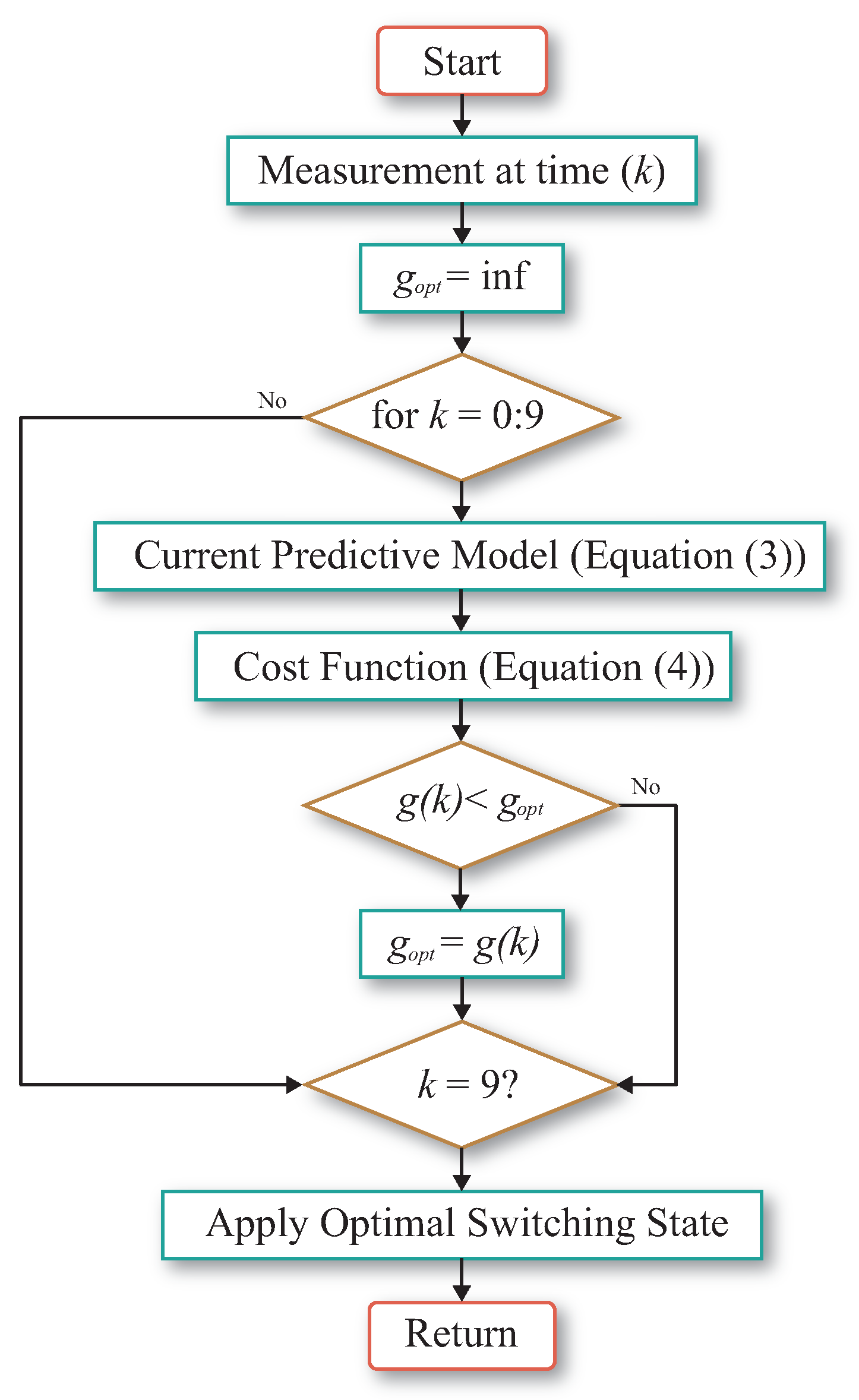
The summary of the predictive control strategy is depicted in the block diagram shown in Figure 5 and the flowchart of this strategy is represented in Figure 6. In this case, a current control is performed by the single-phase output; for this reason, it is essential to define the mathematical model of the load, represented by

$$\frac{d{i}_o}{dt}=\frac{1}{L}{v}_o-\frac{R}{L}{i}_o$$

(1)

However, Equation (1) is in the continuous time and this controller will be programmed into a digital processor which works under a discrete duty cycle, so the model in Equation (1) must be discrete. Using Euler’s numerical integration method to solve differential equations, approximate discretization is achieved.

$$\frac{d{i}_o}{dt}\cong \frac{i_o[k+1]+i_o\left[k\right]}{T_s}$$

(2)

$$i_o^j[k+1]=\frac{T_s}{L}{v}_o^j\left[k\right]+\left(1-\frac{R{T}_s}{L}\right)i_o\left[k\right]$$

(3)

where

$i_o\left[k\right]$	load current at instant k,
$v_o^j\left[k\right]$	load voltage at instant k for the state j,
$i_o^j[k+1]$	load current at instant k for the state j,
$T_s$	Sampling period,
L	Load inductance,
R	Load resistance.

4.2. Cost Function

The cost function seeks to optimize the variable to be controlled by the system, in order to minimize the costs generated by control actions. In this case, it is desirable that the load current of the converter follows a reference with certain characteristics such as magnitude, frequency, and waveform. Consequently, it is expected that the output current $i_o$ tracks the reference $i_{ref}$; therefore, a cost function that meets this requirement is the error between the reference current and the predicted current in the load:

$$g^j[k+1]={(i_{ref}\left[k\right]-i_o^j[k+1])}^2$$

(4)

Equation (4) describes the quadratic error between the predicted load current for the state j (see Table 1) and the load current reference, which is the cost function to be used in this analysis. This choice of cost function is made to its rapid calculation in microcontrollers and its accuracy in estimating the error. Certainly, the use of absolute error would rightly comply with desired tracking condition. However, this calculation algorithm requires a longer computational processing time (critical for this control). Finally, the cost function will be minimized by a search of the vector to be applied that best minimizes the error between the above mentioned currents.

5. Simulation and Experimental Results

Simulations of the two control strategies were performed using the Gecko Circuits ETH environment. This analysis considered a static load of the resistive-inductive type and was fed by a programmable source of pure sinusoidal signal without offset or amplitude change between phases. The different parameters applied to the simulation tests are presented in

Table 3. Simulation parameters.

Variable	Description	Valor
$v_i$	Source voltage	100 Vpk
$f_i$	Source frequency	50 Hz
$f_s$	Sampling frequency	10 kHz–40 kHz
R	Resistive load	10 $\mathsf{\Omega }$
L	Inductive load	10 mH
$i_o$	Reference amplitude	6 Apk
$f_o$	Reference frequency	50 Hz

. It is important to mention that all the results were performed at a sampling rate of 40 kHz. The color palette used throughout the paper analysis of the article refers to different variables. Thus, the blue color identifies the load current, red the load voltage, and green the input voltage.

5.1. Steady-State Analysis

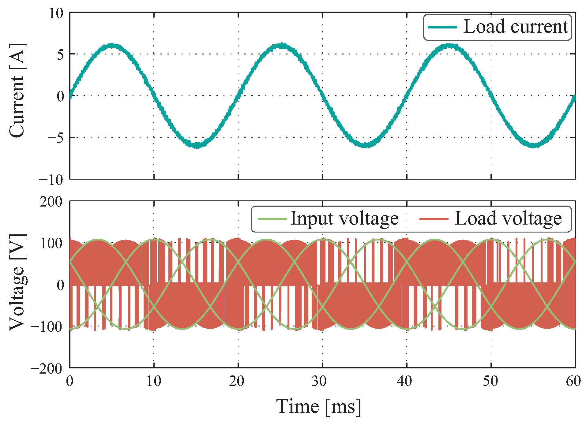
The first test of the controllers considers steady-state analysis. In Figure 7, the results for the SPWM+PI control are displayed where the reference is tracked with low steady-state error. When zooming in on the load current, it is observed that the ripple around the output current is homogeneous; there are no large peaks along the response.

The basis lies in how the PID controller operates which between point and point generates a line with a stable slope formed from the chosen values of the proportional, integral, and derivative constants.

Figure 8 represents the results obtained for the model based on predictive control strategy in the SPMC. This control is highlighted for being simple to implement with rapid dynamic response to input or reference changes. The model is composed of two equations which are integrated into a small code with only nine valid switching states. Therefore, if there is an offset, amplitude differences or changes in the shape of the three-phase input lines, the predictive control applied to this SPMC will still get an optimal tracking.

When comparing Figure 7 with Figure 8, it is possible to identify certain traits typical of the controller type. A clear difference in switching density is observed on the voltage graph. While both share a sampling rate of 40 kHz, the amount of switching by the MPC control is higher. This is further evident by zooming in on the current graph, where it is identified that the ripple generated by the SPWM+PID controller has a greater amplitude. Thus, under this analysis in MPC it turns out to keep a better track of the reference at the cost of increasing the number of switching, this leads to a lower efficiency caused by switching losses.

5.2. Transient State Analysis

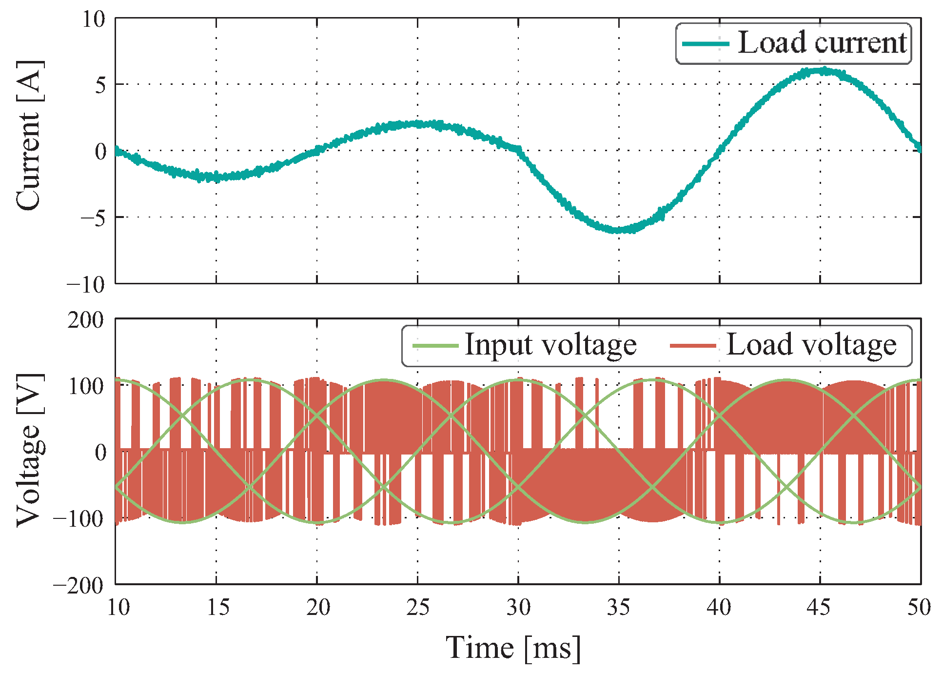
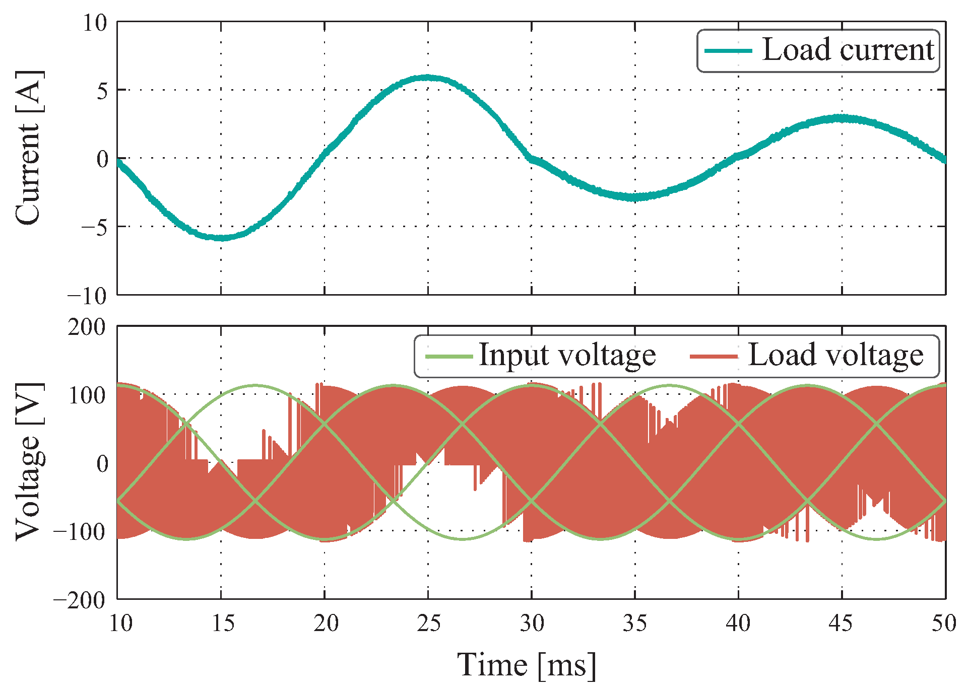
A second test evaluates the dynamic response presented by both controllers. The test consists of generating an amplitude step by moving from the 3 A to 6 A peak current in the reference without varying the output frequency. Thus, on the one hand, Figure 9 shows the results for the SPWM+PI control, and on the other hand Figure 10 the results generated by the MPC under ideal conditions.

In both cases, the dynamic response is fast and the trace frames a minimum steady state error. However, if we look at it in detail, the results for the SPWM+PI control have a higher ripple circularly, which is minimal for the MPC case. For load voltage shown in Figure 10, a higher switching density can be observed when working with the MPC compared to what is seen in the modulation.

The comparison in the response offered by both controllers to a step change is interesting to address. Under the simulation environment, several tests were performed to monitor the speed of the transient response. The results show that the MPC is faster at reaching steady state with an average speed of 250 $\mathsf{\mu }$s over the PID+SPWM control with 1380 $\mathsf{\mu }$s. This demonstrates the robustness of predictive control against abrupt changes in the reference and in turn supports the comments in the analysis of responses in a steady state.

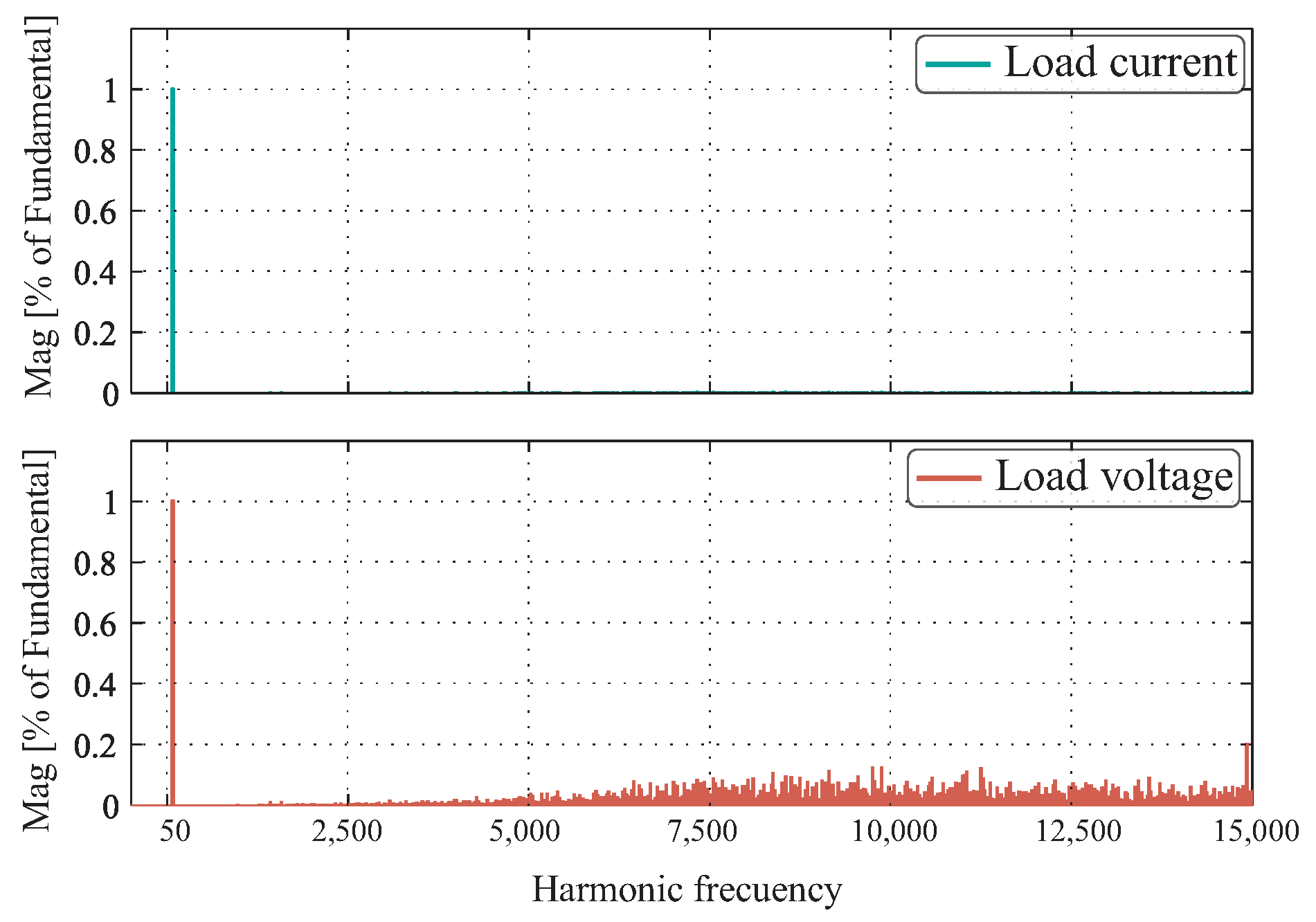
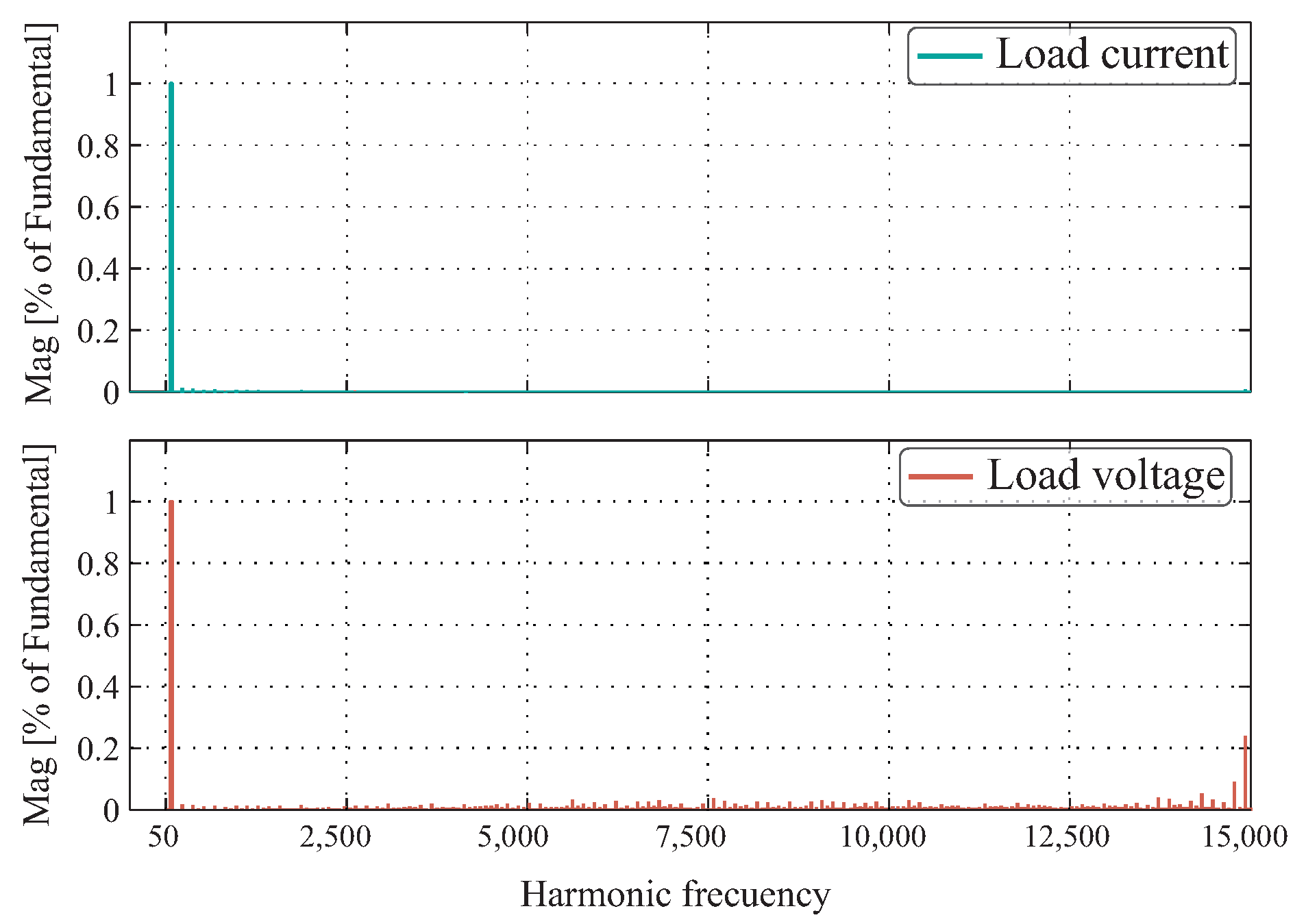
5.3. Harmonic Analysis

Figure 11 shows the resulting harmonic distribution under the PID+SPWM controller tests, and Figure 12 shows the resulting harmonic distribution for the MPC control technique. In both cases, the graphs demonstrate a clear presence of the fundamental with low harmonic distortion. When evaluating the response for the load current, the harmonics do not represent a significant amplitude. However, under the analysis of load voltages, there is a distributed spectrum, mainly in the control PID+SPWM. Considering that total harmonic distortion (THD) represents a measure of distortion that relates the effective values of harmonics to the fundamental frequency, it can be said that 2.341% THD is obtained for PID+SPWM and 2.376% THD for MPC with respect to the load current. The distribution of harmonics outside the fundamental is minimal and extends over a wide frequency range.

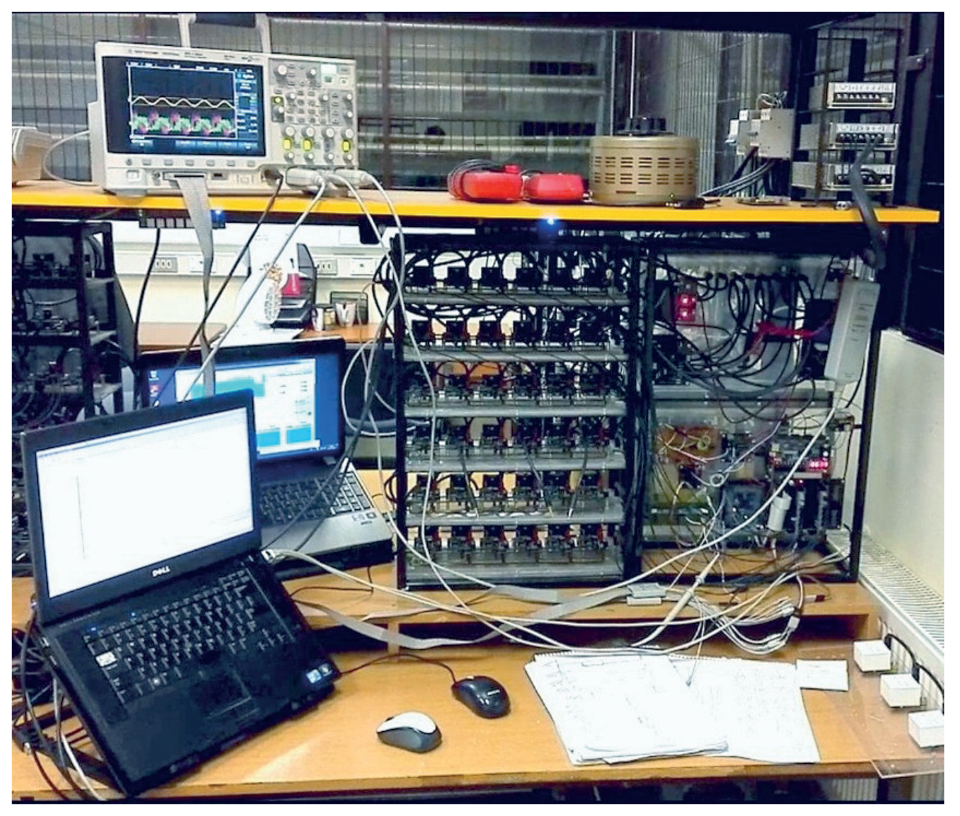
5.4. Experimental Results

Table 4. Laboratory resources.

Resource	Model
Source	Programmable 6 kVA three-phase Chroma 61704
Switch	IGBT FGH80N60FD + driver HCPL3120
Load	Resistance 10 $\mathsf{\Omega }$ + inductance 10 H
Controller	DSC Texas Instruments TMS320F28335
Commutation	FPGA Spartan-3 XC3S1200E-4FTG256C
Protection	Clamp circuit 2 kW

lists the equipment and parameters used for the experimental analysis (Figure 13). The experimental results are obtained under the same conditions as the scenario proposed in the simulations. That is, with an $RL$ load, same input voltage and switching frequency of the devices. However, in the experimental work, a four-step switching commutation was programmed in a FPGA algorithm required to perform a secure switching between the switches that form a matrix converter.

This adds an extra delay to semiconductor switching when considering a time of 2 $\mathsf{\mu }$s per step. To make these relevant aspects obvious when comparing the results, we proceed to analyze the results obtained with a sampling frequency of 40 kHz.

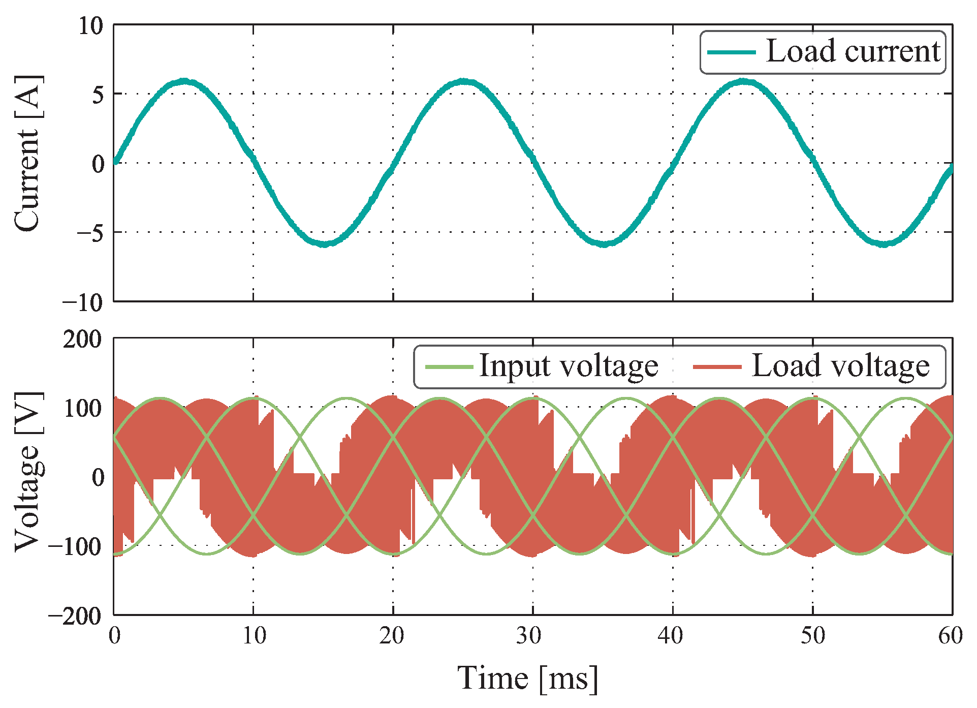
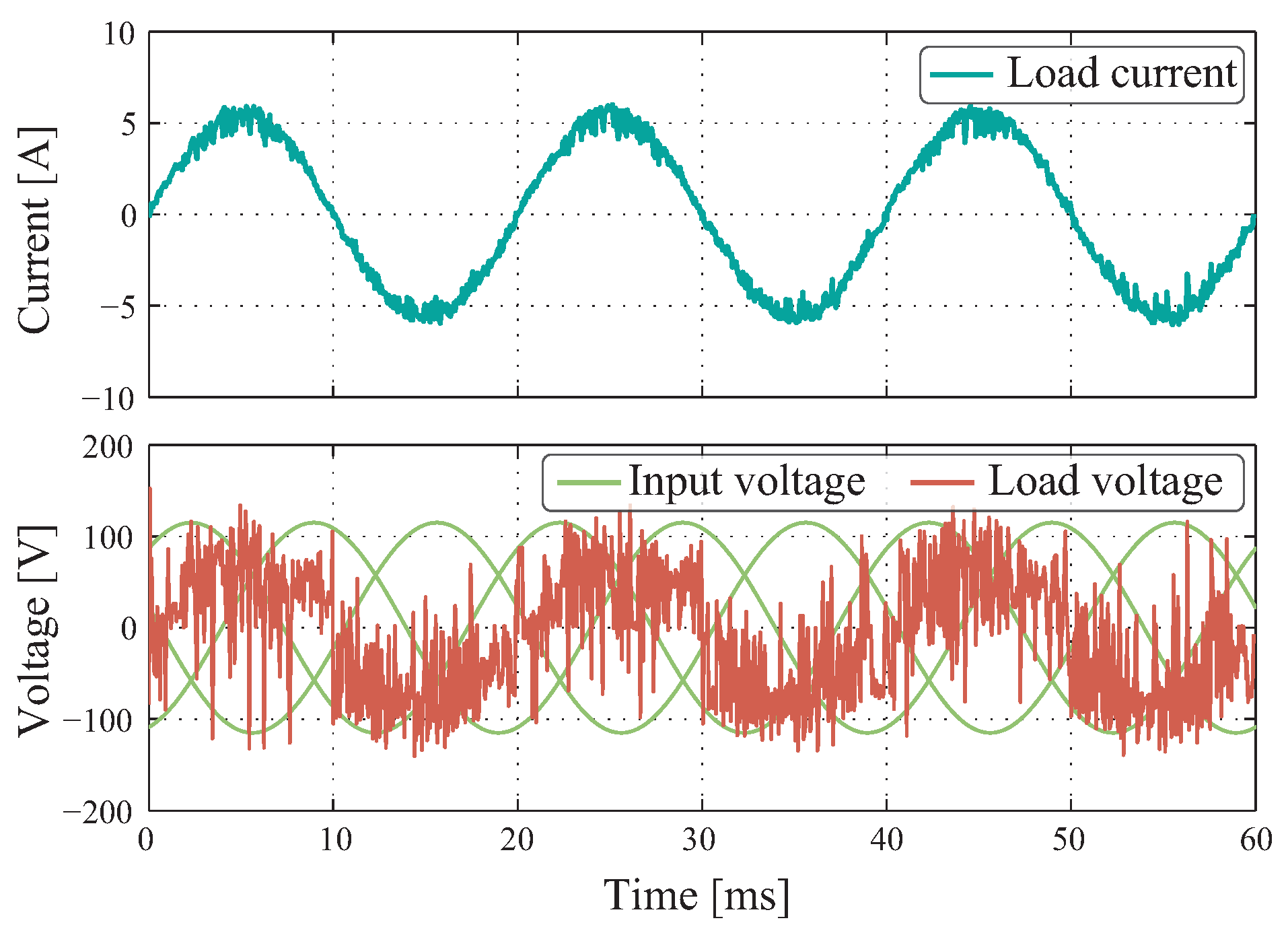
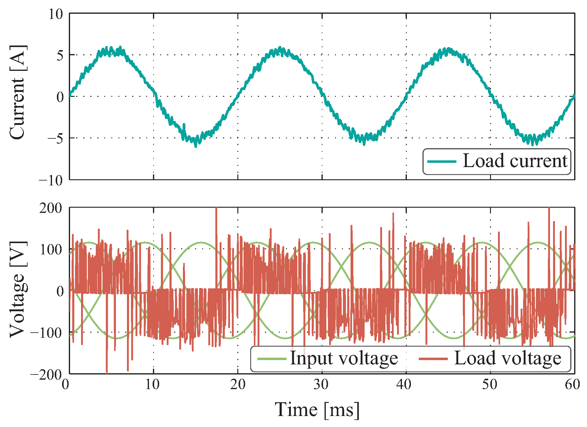
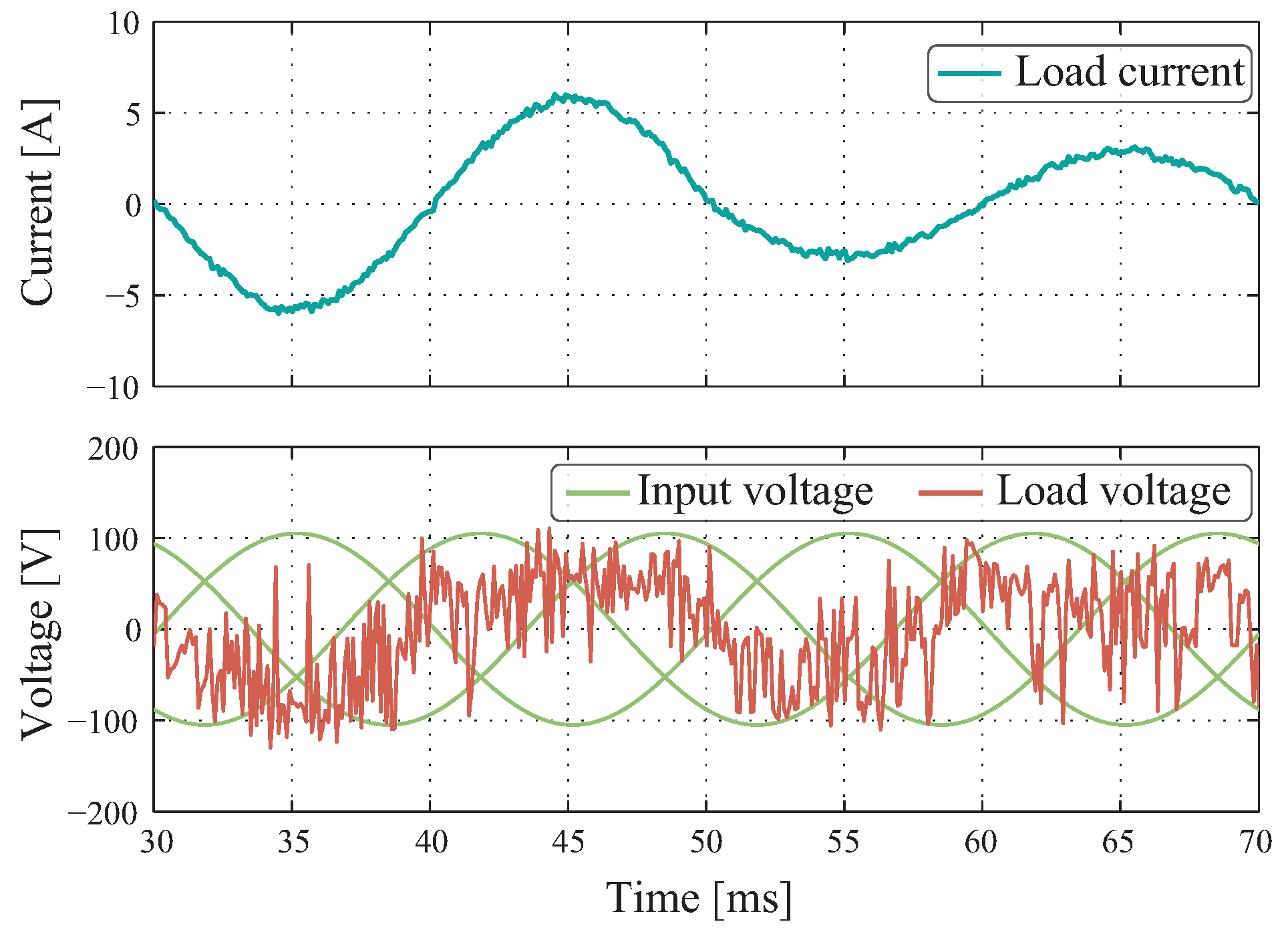
Figure 14 shows the result when implementing SPWM for the SPMC. In contrast to Figure 7, one can observe that there is a higher current ripple produced by the implementation of the switching strategy. Despite this, the tracking to the load current reference meets the controller’s primary goal. Figure 15 shows the behavior of predictive control under experimental conditions. The output current effectively forms a 6 A amplitude sinusoidal with an output frequency of 50 Hz accomplishing a good tracking to its respective reference. Unlike the simulation, the experiments present an increment in ripple, which is due to the commutation of the switches, and also because the load parameters are not exact. Unlike the SPWM method, in this case, higher ripple in comparison to the simulation results is also observed.

The data collected show an average difference of 6.65% between the simulation and experimental results of the PID+SPWM, and 2.21% between the simulation and experimental results with MPC. In addition, there is an average difference under 1.09% simulation between the two controls, and an average difference of 5.53% under experimentation between both controllers in a laboratory environment.

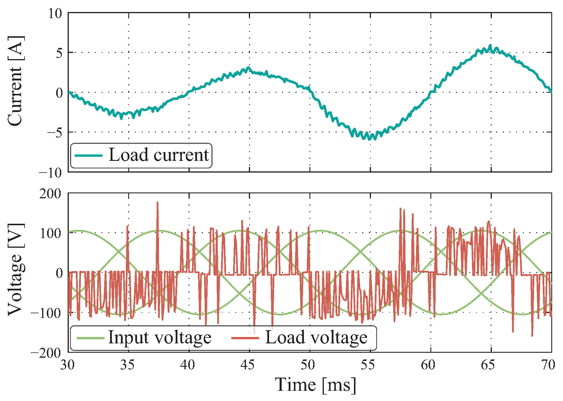
To provide consistency in our methodical analysis, it was possible to measure the delay in reaching the reference that both controllers have when operating in a transient state. When comparing Figure 16 with what was obtained by simulation in Figure 9, it can be said that on average, the PID+SPWM takes 1380 $\mathsf{\mu }$s to go back to the steady state versus the 1540 $\mathsf{\mu }$s that it takes in the experimental results. Similarly, for the MPC strategy, when operating under transient state applying a 3 to 6 A step reference in simulation (Figure 10) takes 250 $\mathsf{\mu }$s versus in laboratory tests (Figure 17) where on average it achieves 390 $\mathsf{\mu }$s. Visually, over-cushioning in the output current can be seen using the PID+SPWM technique. However, the MPC method does not have it, but rather once it reaches the reference it remains in a steady state.

When performing an analysis of harmonics developed under the THD indicator in the output current, there is an average difference of 5.22% between the simulation and experimentation for the PID+SPWM control, and 3.48% between simulation and experimentation for the MPC technique. There is an average difference under simulation of 1.19% between both controllers, and an average difference 3.77% between them in the experiments. As in the case of error, the THD in the output current decreases progressively as the sampling rate and the amplitude of the current increases, except in the experimental case where there is a variability in the decrease in the response of the used electronic components.

6. Conclusions

In this paper, two control techniques for the single-phase matrix converter (SPMC) have been presented, showing a comparison by simulation and experimental results between them. Both techniques are easy to implement on a digital microcontroller and generate good tracking in respect to references. The simplicity and good performance of these strategies allows them to be widely recommended for any matrix converter topology.

The same parameters have been considered for both the simulation and experimental evaluation. However, a four-step switching commutation strategy was also required for the experimental implementation in order to ensure the safe operation of the converter’s switches. In addition, for both methods, a higher ripple in the load current is observed in the experimental implementation in comparison to the simulations. This is mainly due to the commutation of the switches, but also to some uncertainties in the load parameters. For the PID+SPWM, an average difference of 6.65% between the simulation and experimental results was observed. For the MPC, the average difference is 2.21%, which is significant.

Experimental tests have shown that the quality of the current source at the output is directly related to the voltage stability at the input source. Then, to ensure the good tracking of the current required by the controllers, it is necessary that the calculated voltage is in the operating region demarcated by the crossing of the phase lines.

The two shown methods have high performance, and the choice of which one to use will depend on the required application. Thus, for better current tracking at the cost of increased switching losses, the choice tends toward predictive control. On the other hand, a significant decrease in harmonic generation at the cost of less reference tracking would involve choosing the PID+SPWM control.

For the PID+SPWM technique, the main limitation is due to the adjustment of the controller’s parameters which need to be set based on the operation point. In addition, as demonstrated in the simulated and experimental results, the technique takes more time in to reach steady state in comparison to the MPC strategy. For the predictive control technique, the main limitations are the quality of the prediction model and the variable switching frequency operation, which affects the quality of the controller.

Whatever the choice, both techniques offer excellent dynamic response, robustness against external disturbances, and have easy implementations, allowing them to be applied in applications such as radio frequency induction heating which needs high-frequency AC power supply and wireless power transfer systems to high-power coils in vehicle-to-grid among others.

References

- Gyugi, L.; Pelly, B. Static Power Frequency Changers: Theory, Performance and Applications; Wiley: New York, NY, USA, 1976. [Google Scholar]
- Venturini, M. A new sine wave in sine wave out, conversion technique which eliminates reactive elements. Proc. Powercon 1980, 7, E3/1–E3/15. [Google Scholar]
- Alesina, A.; Venturini, M.G.B. Analysis and design of optimum-amplitude nine-switch direct AC-AC converters. IEEE Trans. Power Electron. 1989, 4, 101–112. [Google Scholar] [CrossRef]
- Friedli, T.; Kolar, J.W.; Rodriguez, J.; Wheeler, P.W. Comparative Evaluation of Three-Phase AC–AC Matrix Converter and Voltage DC-Link Back-to-Back Converter Systems. IEEE Trans. Ind. Electron. 2012, 59, 4487–4510. [Google Scholar] [CrossRef]
- Rodriguez, J.; Rivera, M.; Kolar, J.W.; Wheeler, P.W. A Review of Control and Modulation Methods for Matrix Converters. IEEE Trans. Ind. Electron. 2012, 59, 58–70. [Google Scholar] [CrossRef]
- Boonseam, P.; Jarutus, N.; Kumsuwan, Y. A control strategy for a matrix converter based on Venturini method under unbalanced input voltage conditions. In Proceedings of the 2016 13th International Conference on Electrical Engineering/Electronics, Computer, Telecommunications and Information Technology (ECTI-CON), Chiang Mai, Thailand, 28 June–1 July 2016; pp. 1–6. [Google Scholar]
- Rahman, K.; Iqbal, A.; Al-Hitmi, M.A.; Dordevic, O.; Ahmad, S. Performance Analysis of a Three-to-Five Phase Dual Matrix Converter Based on Space Vector Pulse Width Modulation. IEEE Access 2019, 7, 12307–12318. [Google Scholar] [CrossRef]
- Zhang, J.; Yang, H.; Wang, T.; Li, L.; Dorrell, D.G.; Lu, D.D. Field-oriented control based on hysteresis band current controller for a permanent magnet synchronous motor driven by a direct matrix converter. IET Power Electron. 2016, 11, 1277–1285. [Google Scholar] [CrossRef]
- Mubarok, M.S.; Liu, T. Implementation of Predictive Controllers for Matrix-Converter-Based Interior Permanent Magnet Synchronous Motor Position Control Systems. IEEE J. Emerg. Sel. Top. Power Electron. 2019, 7, 261–273. [Google Scholar] [CrossRef]
- Monteiro, J.; Silva, J.F.; Pinto, S.F.; Palma, J. Linear and Sliding-Mode Control Design for Matrix Converter-Based Unified Power Flow Controllers. IEEE Trans. Power Electron. 2014, 27, 3357–3367. [Google Scholar] [CrossRef]
- Yan, Y.; Zhao, J.; Xia, C.; Shi, T. Direct torque control of matrix converter-fed permanent magnet synchronous motor drives based on master and slave vectors. IET Power Electron. 2015, 8, 288–296. [Google Scholar] [CrossRef]
- Hemakesavulu, O.; Subbaiah, P. Simulation and Analysis of Fuzzy Based Modulation Control Technique of Matrix Converter. In Proceedings of the 2018 2nd International Conference on I-SMAC (IoT in Social, Mobile, Analytics and Cloud) (I-SMAC)I-SMAC (IoT in Social, Mobile, Analytics and Cloud) (I-SMAC), Palladam, India, 30–31 August 2018; pp. 438–442. [Google Scholar]
- Lee, H.H.; Dzung, P.Q.; Phuong, L.M.; Khoa, L.D. A new artificial neural network controller for direct control method for matrix converters. In Proceedings of the 2009 International Conference on Power Electronics and Drive Systems (PEDS), Taipei, Taiwan, 2–5 November 2009; pp. 434–439. [Google Scholar]
- Lei, J.; Zhou, B.; Qin, X.; Wei, J.; Bian, J. Active damping control strategy of matrix converter via modifying input reference currents. IEEE Trans. Power Electron. 2015, 30, 5260–5271. [Google Scholar] [CrossRef]
- Zhang, J.; Li, L.; Dorrell, D.G.; Guo, Y. Modified PI controller with improved steady-state performance and comparison with PR controller on direct matrix converters. Chin. J. Electr. Eng. 2019, 5, 53–66. [Google Scholar] [CrossRef]
- Empringham, L.; Kolar, J.W.; Rodriguez, J.; Wheeler, P.W.; Clare, J.C. Technological Issues and Industrial Application of Matrix Converters: A Review. IEEE Trans. Ind. Electron. 2013, 60, 4260–4271. [Google Scholar] [CrossRef]
- Nguyen-Quang, N.; Stone, D.A.; Bingham, C.M.; Foster, M.P. Single phase matrix converter for radio frequency induction heating. In Proceedings of the International Symposium on Power Electronics, Electrical Drives, Automation and Motion (SPEEDAM 2006), Taormina, Italy, 23–26 May 2006; pp. 614–618. [Google Scholar]
- Guan, L.; Wang, Z.; Liu, P.; Wu, J. A Three-Phase to Single-Phase Matrix Converter for Bidirectional Wireless Power Transfer System. In Proceedings of the IECON 2019—45th Annual Conference of the IEEE Industrial Electronics Society, Lisbon, Portugal, 14–17 October 2019; pp. 4451–4456. [Google Scholar]
- Venugopal, L.V.; Jayapal, R. Matrix converter based energy saving for street lights. In Proceedings of the 2015 International Conference on Circuits, Power and Computing Technologies [ICCPCT-2015], Nagercoil, India, 19–20 March 2015; pp. 1–6. [Google Scholar]
- Wheeler, P.W.; Rodriguez, J.; Clare, J.C.; Empringham, L.; Weinstein, A. Matrix converters: A technology review. IEEE Trans. Ind. Electron. 2002, 49, 276–288. [Google Scholar] [CrossRef]
- Rojas, C.; Rodriguez, J.; Iqbal, A.; Abu-Rub, H.; Wilson, A.; Ahmed, S.M. A simple modulation scheme for a regenerative Cascaded Matrix Converter. In Proceedings of the 37th Annual Conference of the IEEE Industrial Electronics Society (IECON 2011), Melbourne, Australia, 7–10 November 2011; pp. 4361–4366. [Google Scholar]
- Toledo, S.; Gregor, R.; Rivera, M.; Rodas, J.; Gregor, D.; Caballero, D.; Gavilán, F.; Maqueda, E. Multi-modular matrix converter topology applied to distributed generation systems. In Proceedings of the 8th IET International Conference on Power Electronics, Machines and Drives (PEMD 2016), Glasgow, UK, 19–21 April 2016; pp. 1–6. [Google Scholar]
- Olloqui, A.; Elizondo, J.L.; Rivera, M.; Macias, M.E.; Micheloud, O.M.; Pena, R.; Wheeler, P. Indirect power control of a DFIG using model-based predictive rotor current control with an indirect matrix converter. In Proceedings of the 2015 IEEE International Conference on Industrial Technology (ICIT), Seville, Spain, 17–19 March 2015; pp. 2275–2280. [Google Scholar]
Figure 1.
Single-phase matrix converter 3 × 2.
Figure 2.
Unipolar modulation scheme.
Figure 3.
Three-phase source sectoring. (a) binary comparators to frame the different sectors, (b) sectoring of the input source.
Figure 4.
Integrated control scheme PID+SPWM.
Figure 5.
Predictive control scheme.
Figure 6.
Flowchart predictive control applied.
Figure 7.
Simulation results in steady state for SPMW+PID control with reference from 6 A to 50 Hz and a sampling rate of 40 kHz.
Figure 8.
Simulation results in steady state for Model-based Predictive Control (MPC) with reference from 6 A to 50 Hz and a sampling frequency of 40 kHz.
Figure 9.
Simulation results under transient regime for SPMW+PID control with reference from 3 A to 6 A to 50 Hz and a sampling frequency of 40 kHz.
Figure 10.
Simulation results under transient regime for MPC control with reference from 6 A to 3 A to 50 Hz and a sampling frequency of 40 kHz.
Figure 11.
Harmonic spectrum for SPMW+PID control under simulation environment.
Figure 12.
Harmonic spectrum for MPC under simulation environment.
Figure 13.
Experimental set-up.
Figure 14.
Experimental results in steady state for SPMW+PID control with reference from 6 A to 50 Hz and a sampling rate of 40 kHz.
Figure 15.
Experimental results in steady state for MPC control with reference from 6 A to 50 Hz and a sampling rate of 40 kHz.
Figure 16.
Experimental results under transient regime for SPMW+PID control with reference from 3 A to 6 A to 50 Hz and a sampling frequency of 40 kHz.
Figure 17.
Experimental results under transitional regime for MPC control with reference from 6 A to 3 A to 50 Hz and a sampling frequency of 40 kHz.