Recent Progress in Hydrogen Flammability Prediction for the Safe Energy Systems


Abstract
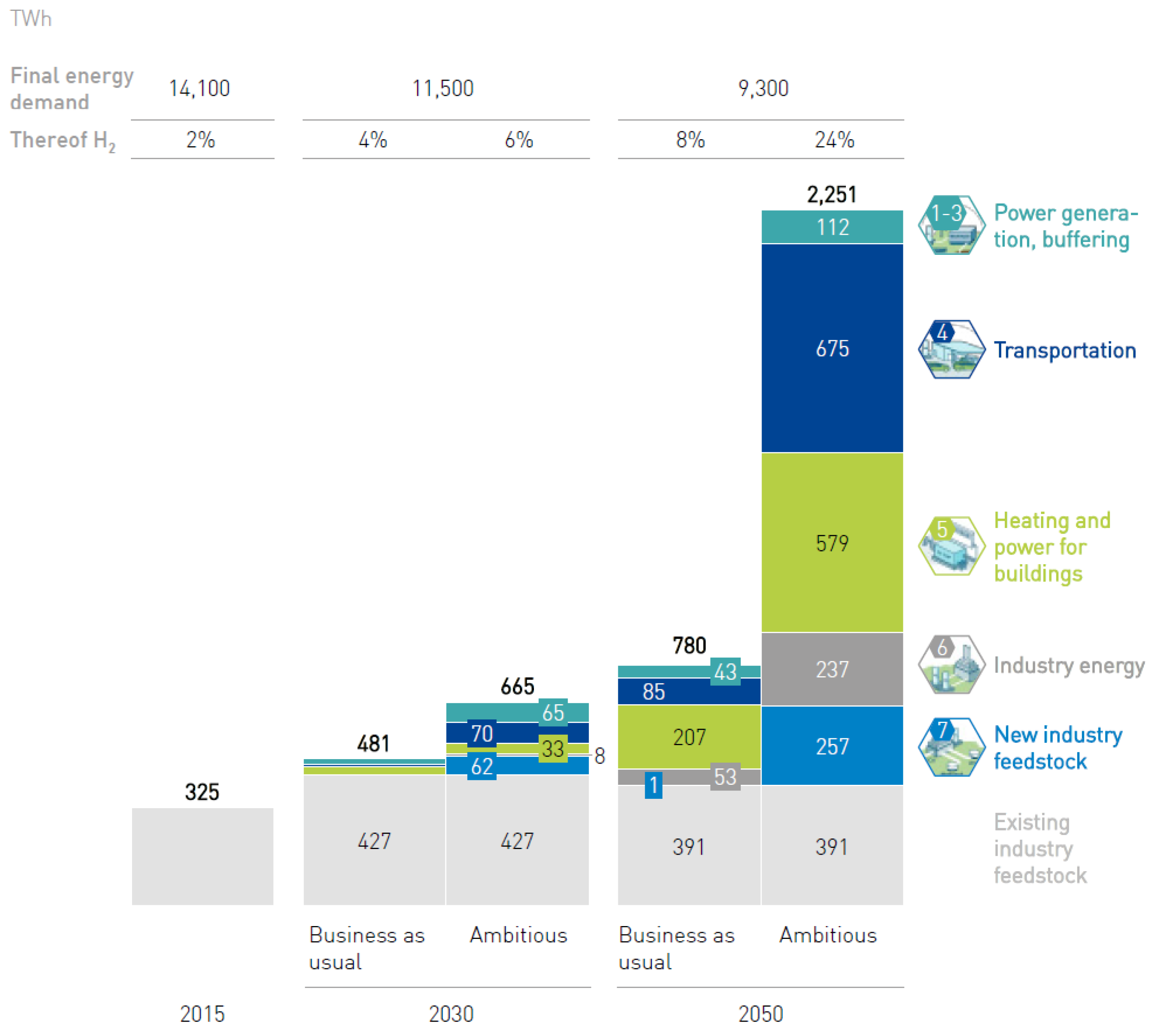
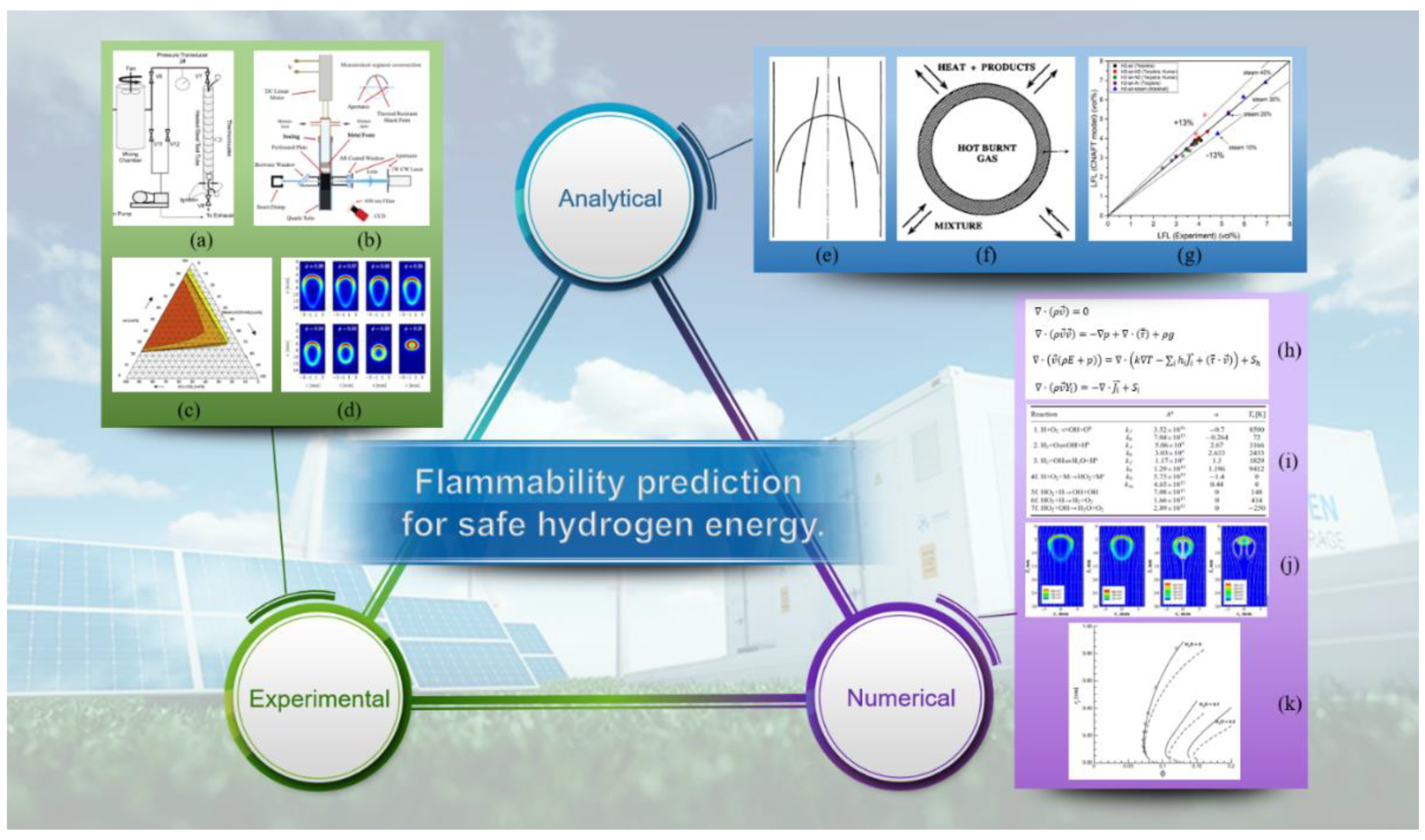
1. Introduction
2. Experimental Studies
2.1. Flame Propagation Experiments to Measure the Flammability Limit
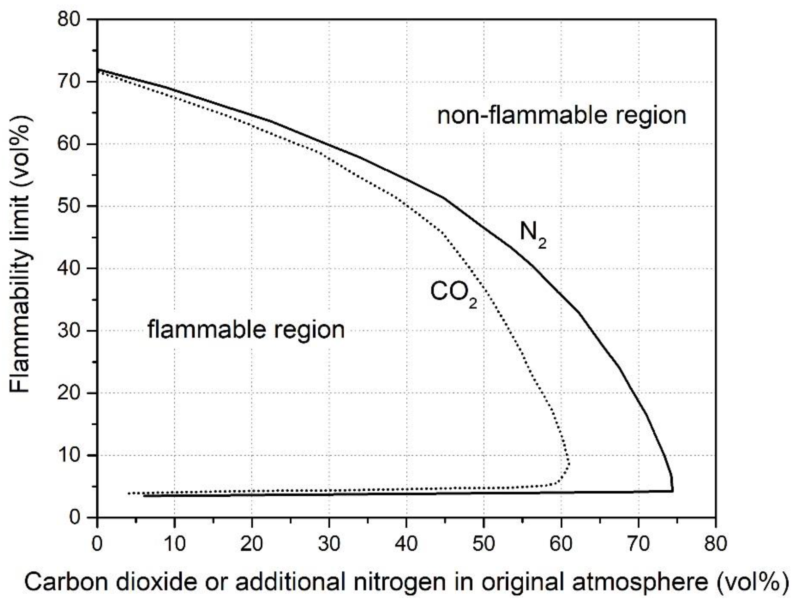
2.2. Diluent Effects
2.3. Elevated Temperature and Pressure
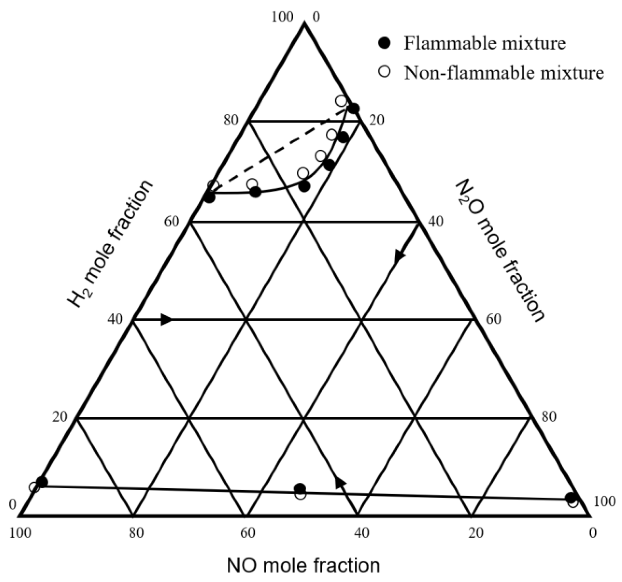
2.4. Binary Fuels and Diluents
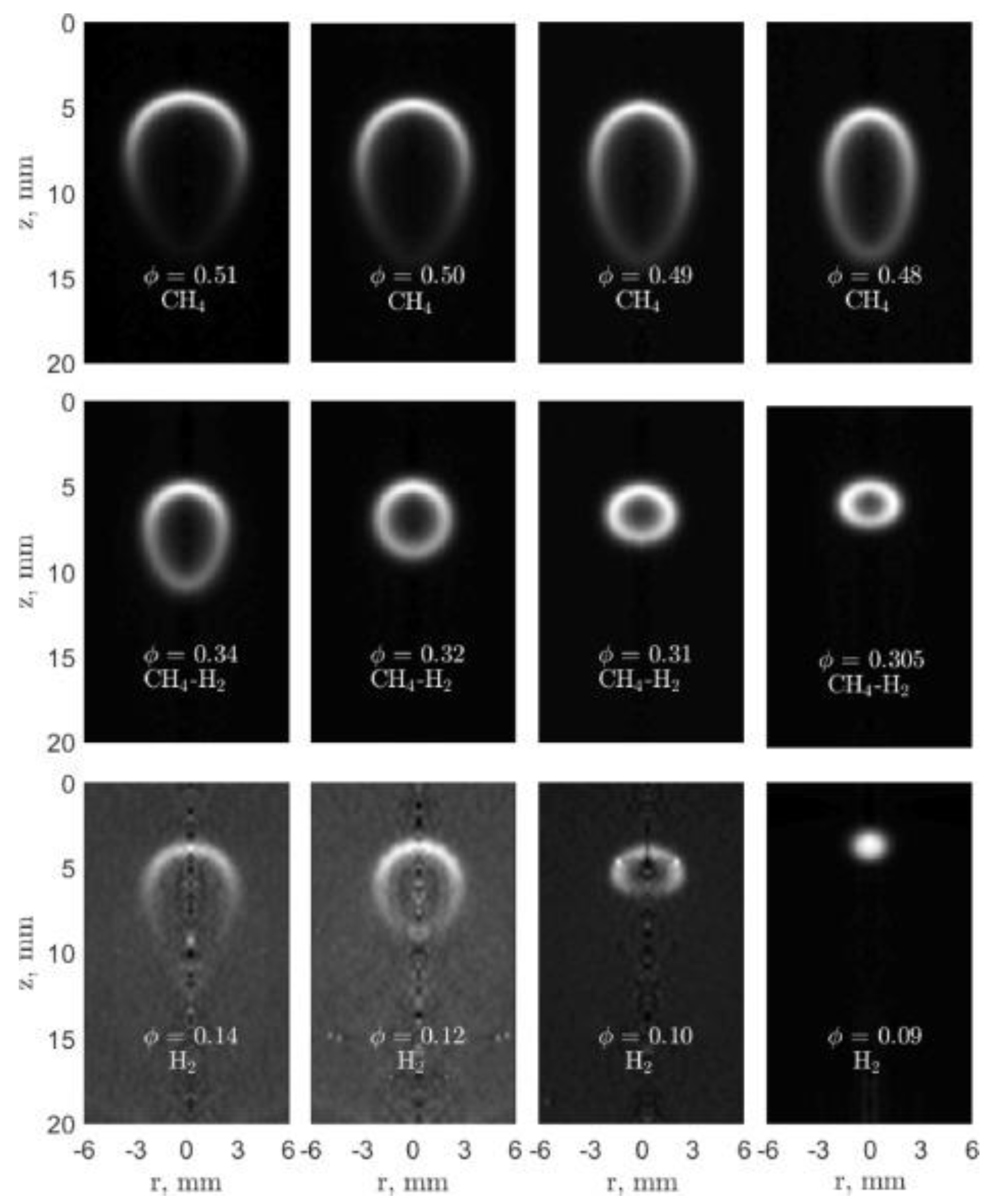
2.5. Flame Ball and Counterflow Flame
3. Numerical Studies
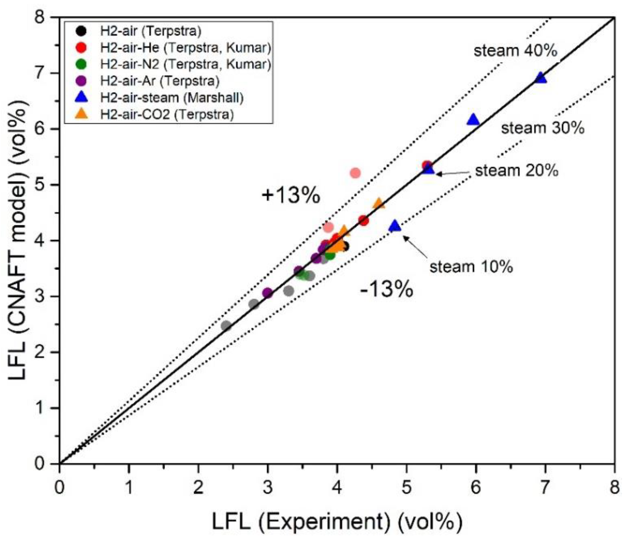
3.1. Propagating Flame Simulations
3.2. Stationary Flame Ball
3.3. Counterflow Flame
4. Analytical Studies
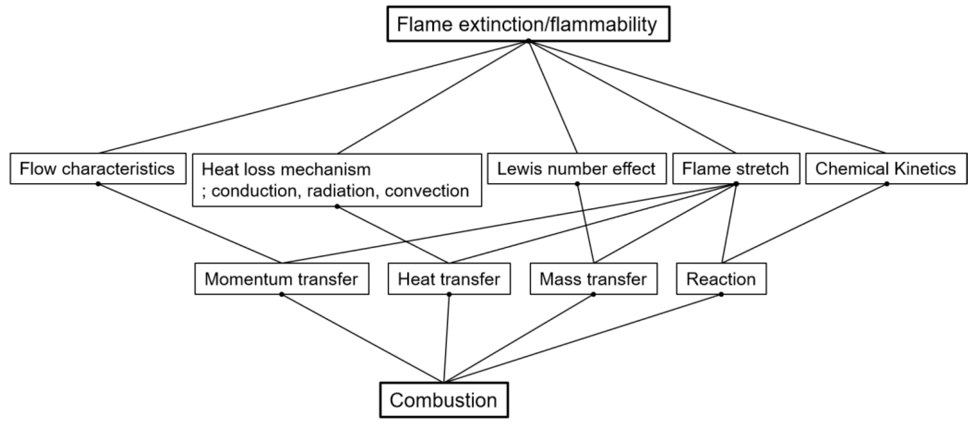
4.1. Systemic Combustion Analysis
4.2. Analytical Analyses of Propagating Flame
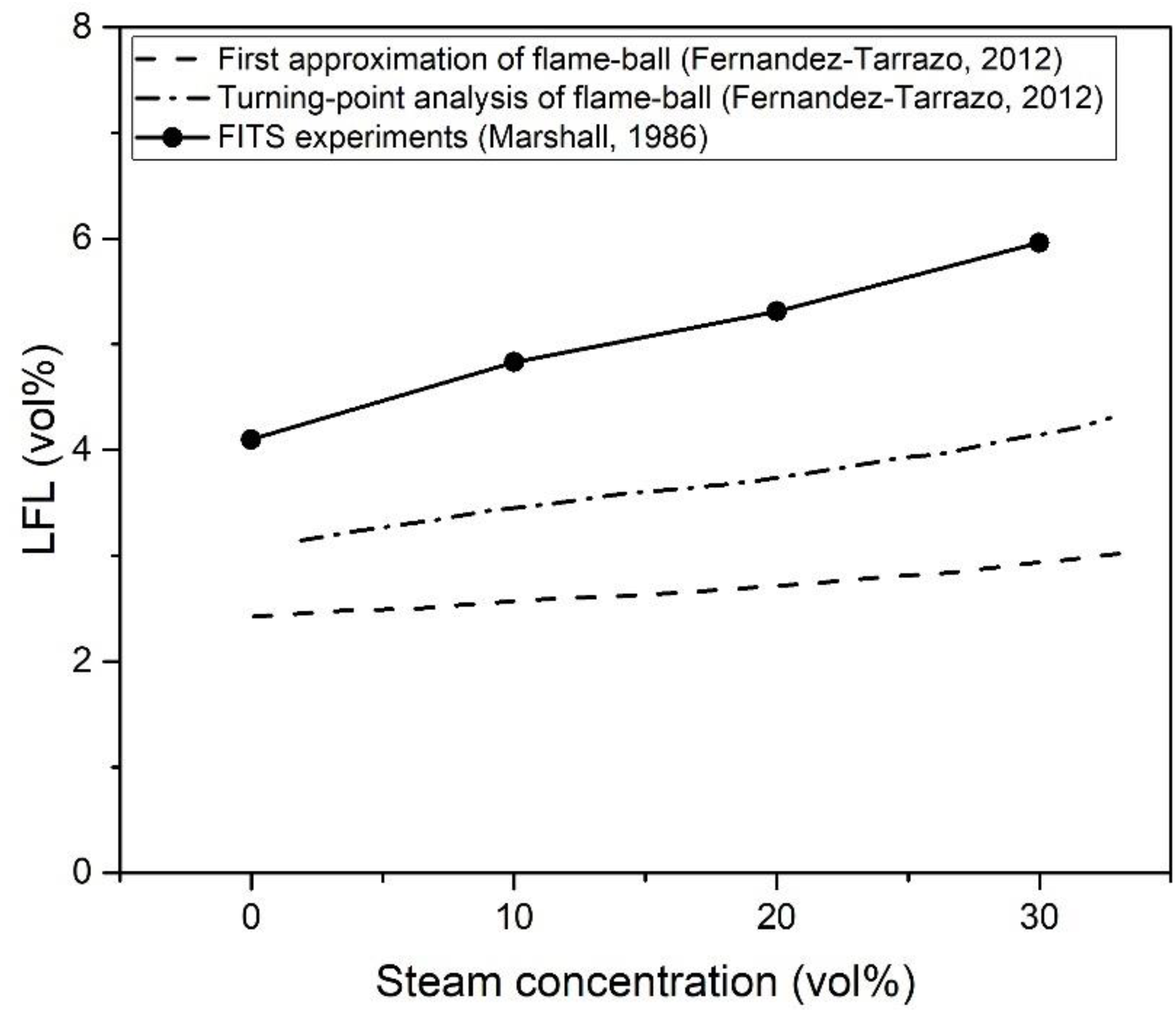
4.3. Flame Ball Analyses
5. Concluding Remarks
Author Contributions
Funding
Conflicts of Interest
References
- Fuel Cells and Hydrogen Joint Undertaking (FCHJU). Hydrogen Roadmap Europe; Fuel Cells and Hydrogen Joint Undertaking: Bietlot, Belgium, 2019. [Google Scholar]
- Kim, J.H.; Kim, H.J.; Yoo, S.H. Willingness to pay for fuel-cell electric vehicles in South Korea. Energy 2019, 174, 497–502. [Google Scholar] [CrossRef]
- Molnarne, M.; Schroeder, V. Hazardous properties of hydrogen and hydrogen containing fuel gases. Process Saf. Environ. 2019, 130, 1–5. [Google Scholar] [CrossRef]
- Kim, N.K.; Jeon, J.; Choi, W.; Kim, S.J. Systematic hydrogen risk analysis of OPR1000 containment before RPV failure under station blackout scenario. Ann. Nucl. Energy 2018, 116, 429–438. [Google Scholar] [CrossRef]
- Sarikurt, F.S.; Hassan, Y.A. Large eddy simulations of erosion of a stratified layer by a buoyant jet. Int. J. Heat Mass Trans. 2017, 112, 354–365. [Google Scholar] [CrossRef]
- Bauer, C.; Forest, T. Effect of hydrogen addition on the performance of methane-fueled vehicles. Part I: Effect on SI engine performance. Int. J. Hydrogen Energy 2001, 26, 55–70. [Google Scholar] [CrossRef]
- Wierzba, I.; Kilchyk, V. Flammability limits of hydrogen–carbon monoxide mixtures at moderately elevated temperatures. Int. J. Hydrogen Energy 2001, 26, 639–643. [Google Scholar] [CrossRef]
- Nikolaidis, P.; Poullikkas, A. A comparative overview of hydrogen production processes. Renew. Sustain. Energy Rev. 2017, 67, 597–611. [Google Scholar] [CrossRef]
- Ciccarelli, G.; Dorofeev, S. Flame acceleration and transition to detonation in ducts. Prog. Energy Combust. 2008, 34, 499–550. [Google Scholar] [CrossRef]
- Mayer, E. A theory of flame propagation limits due to heat loss. Combust. Flame 1957, 1, 438–452. [Google Scholar] [CrossRef]
- Jeon, J.; Choi, W.; Kim, S.J. A flammability limit model for hydrogen-air-diluent mixtures based on heat transfer characteristics in flame propagation. Nucl. Eng. Technol. 2019, 51, 1749–1757. [Google Scholar] [CrossRef]
- Sánchez, A.L.; Williams, F.A. Recent advances in understanding of flammability characteristics of hydrogen. Prog. Energy Combust. 2014, 41, 1–55. [Google Scholar] [CrossRef]
- Von Lavante, E.; Strehlow, R.A. The mechanism of lean limit flame extinction. Combust. Flame 1983, 49, 123–140. [Google Scholar] [CrossRef]
- Coward, H.F.; Jones, G.W. Limits of Flammability of Gases and Vapors; Bureau of Mines: Washington, DC, USA, 1952.
- Terpstra, M. Flammability Limits of Hydrogen-Diluent Mixtures in Air. Master’s Thesis, University of Calgary, Calgary, AB, Canada, 2012. [Google Scholar]
- Zhou, Z.; Shoshin, Y.; Hernández-Pérez, F.E.; Van Oijen, J.A.; De Goey, L.P. Experimental and numerical study of cap-like lean limit flames in H2-CH4-air mixtures. Combust. Flame 2018, 189, 212–224. [Google Scholar] [CrossRef]
- Bentaib, A.; Meynet, N.; Bleyer, A. Overview on hydrogen risk research and development activities: Methodology and open issues. Nucl. Eng. Technol. 2015, 47, 26–32. [Google Scholar] [CrossRef]
- Hernández-Pérez, F.E.; Oostenrijk, B.; Shoshin, Y.; Van Oijen, J.A.; De Goey, L.P. Formation, prediction and analysis of stationary and stable ball-like flames at ultra-lean and normal-gravity conditions. Combust. Flame 2015, 162, 932–943. [Google Scholar] [CrossRef]
- Buckmaster, J.; Mikolaitis, D. A flammability-limit model for upward propagation through lean methane/air mixtures in a standard flammability tube. Combust. Flame 1982, 45, 109–119. [Google Scholar] [CrossRef]
- Buckmaster, J.; Smooke, M.; Giovangigli, V. Analytical and numerical modeling of flame-balls in hydrogen-air mixtures. Combust. Flame 1993, 94, 113–124. [Google Scholar] [CrossRef]
- Fernández-Galisteo, D.; Sánchez, A.L.; Liñán, A.; Williams, F.A. The hydrogen–air burning rate near the lean flammability limit. Combust. Theory Model 2009, 13, 741–761. [Google Scholar] [CrossRef]
- Zhou, Z.; Shoshin, Y.; Hernandez-Perez, F.E.; Van Oijen, J.A.; De Goey, L.P. Effect of Lewis number on ball-like lean limit flames. Combust. Flame 2018, 188, 77–89. [Google Scholar] [CrossRef]
- Fernández-Tarrazo, E.; Sánchez, A.L.; Liñán, A.; Williams, F.A. Flammability conditions for ultra-lean hydrogen premixed combustion based on flame-ball analyses. Int. J. Hydrogen Energy 2012, 37, 1813–1825. [Google Scholar] [CrossRef]
- Kazakov, K.A. Premixed flame propagation in vertical tubes. Phys. Fluids 2016, 28, 042103. [Google Scholar] [CrossRef]
- White, A.G. Limits for the propagation of flame in inflammable gas-air mixtures. Part I. Mixtures of air and one gas at the ordinary temperature and pressure. J. Chem. Soc. 1924, 125, 2387–2396. [Google Scholar] [CrossRef]
- Egerton, A.C.; Powling, J. The limits of flame propagation at atmospheric pressure II. The influence of changes in the physical properties. Proc. R. Soc. Lond. A 1948, 193, 190–209. [Google Scholar]
- Jones, G.W. Inflammability of Mixed Gases; US Government Printing Office: Washington, DC, USA, 1929.
- Burgoyne, J.; Williams-Leir, G. The influence of incombustible vapours on the limits of inflammability of gases and vapours in air. Proc. R. Soc. Lond. A 1948, 193, 525–539. [Google Scholar]
- Clusius, K.; Gutschmidt, H. Die untere Explosionsgrenze der Gemische von schwerem Wasserstoff mit Luft. Naturwissenschaften 1934, 22, 693. [Google Scholar] [CrossRef]
- Payman, W. The propagation of flame in complex gaseous mixtures. Part I. Limit mixtures and the uniform movement of flame in such mixtures. J. Chem. Soc. 1919, 115, 1436–1445. [Google Scholar] [CrossRef]
- Van Den Schoor, F. Influence of Pressure and Temperature on Flammability Limits of Combustible Gases in Air. Ph.D. Thesis, Katholieke Universiteit Leuven, Flanders, Belgium, 2007. [Google Scholar]
- Scott, F.; Van Dolah, R.; Zabetakis, M. The flammability characteristics of the system H2-NO-N2O-Air. Proc. Combust. Inst. 1957, 6, 540–545. [Google Scholar] [CrossRef]
- Shebeko, Y.N.; Iliin, A.; Ivanov, A. An experimental investigation of flammability limits in mixtures of hydrogen–oxygen–diluent. J. Chem. Soc. 1984, 58, 862–865. [Google Scholar]
- Kumar, R. Flammability limits of hydrogen-oxygen-diluent mixtures. J. Fire Sci. 1985, 3, 245–262. [Google Scholar] [CrossRef]
- Marshall, B.W. Hydrogen: Air: Steam Flammability Limits and Combustion Characteristics in the FITS Vessel; Sandia National Laboratories: Albuquerque, NM, USA, 1986.
- Hustad, J.E.; Sønju, O.K. Experimental studies of lower flammability limits of gases and mixtures of gases at elevated temperatures. Combust. Flame 1988, 71, 283–294. [Google Scholar] [CrossRef]
- Shebeko, Y.N.; Tsarichenko, S.G.; Korolchenko, A.Y.; Trunev, A.V.; Navzenya, V.Y.; Papkov, S.N.; Zaitzev, A.A. Burning velocities and flammability limits of gaseous mixtures at elevated temperatures and pressures. Combust. Flame 1995, 102, 427–437. [Google Scholar] [CrossRef]
- Ale, B.B. Flammability Limits of Gaseous Fuels and Their Mixtures in Air at Elevated Temperatures. Ph.D. Thesis, University of Calgary, Calgary, AB, Canada, 1998. [Google Scholar]
- Liu, X.; Zhang, Q. Influence of initial pressure and temperature on flammability limits of hydrogen–air. Int. J. Hydrogen Energy 2014, 39, 6774–6782. [Google Scholar] [CrossRef]
- Hu, X.; Xie, Q.; Zhang, J.; Yu, Q.; Liu, H.; Sun, Y. Experimental study of the lower flammability limits of H2/O2/CO2 mixture. Int. J. Hydrogen Energy 2020, 45, 27837–27845. [Google Scholar] [CrossRef]
- Jeon, J.; Kim, Y.S.; Jung, H.; Kim, S.J. A mechanistic analysis of H2O and CO2 diluent effect on hydrogen flammability considering flame extinction mechanism. Nucl. Eng. Technol. Under Review.
- Satterly, J.; Burton, E. Combustibility of Mixtures of Hydrogen and Helium. Trans. R. Soc. Can. 1919, 13, 211–215. [Google Scholar]
- Law, C.; Egolfopoulos, F. A unified chain-thermal theory of fundamental flammability limits. Proc. Combust. Inst. 1992, 24, 137–144. [Google Scholar] [CrossRef]
- Kumar, R.; Tamm, H.; Harrison, W.C. Combustion of hydrogen-steam-air mixtures near lower flammability limits. Combust. Sci. Technol. 1983, 33, 167–178. [Google Scholar] [CrossRef]
- Plys, M.G. Hydrogen production and combustion in severe reactor accidents: An integral assessment perspective. Nucl. Technol. 1993, 101, 400–410. [Google Scholar] [CrossRef]
- Jeon, J.; Choi, W.; Kim, N.K.; Kim, S.J. Numerical investigation of in-vessel core coolability of PWR through an effective safety injection flow model using MELCOR simulation. Ann. Nucl. Energy 2018, 121, 350–360. [Google Scholar] [CrossRef]
- Choi, W.; Yu, S.O.; Kim, S.J. Efficacy analysis of hydrogen mitigation measures of CANDU containment under LOCA scenario. Ann. Nucl. Energy 2018, 118, 122–130. [Google Scholar] [CrossRef]
- Byun, C.; Jerng, D.; Todreas, N.; Driscoll, M. Conceptual design and analysis of a semi-passive containment cooling system for a large concrete containment. Nucl. Eng. Des. 2000, 199, 227–242. [Google Scholar] [CrossRef]
- Martín-Valdepeñas, J.; Jiménez, M.; Martín-Fuertes, F.; Fernández, J. Improvements in a CFD code for analysis of hydrogen behaviour within containments. Nucl. Eng. Des. 2007, 237, 627–647. [Google Scholar] [CrossRef]
- Jeon, J.; Kim, Y.S.; Choi, W.; Kim, S.J. Identification of Hydrogen Flammability in steam generator compartment of OPR1000 using MELCOR and CFX codes. Nucl. Eng. Technol. 2019, 51, 1939–1950. [Google Scholar] [CrossRef]
- Law, C. Propagation, structure, and limit phenomena of laminar flames at elevated pressures. Combust. Sci. Technol. 2006, 178, 335–360. [Google Scholar] [CrossRef]
- Choi, W.; Kim, T.; Jeon, J.; Kim, N.K.; Kim, S.J. Effect of Molten Corium Behavior Uncertainty on the Severe Accident Progress. Sci. Technol. Nucl. Ins. 2018, 2018, 5706409. [Google Scholar] [CrossRef]
- Baird, A.R.; Archibald, E.J.; Marr, K.C.; Ezekoye, O.A. Explosion hazards from lithium-ion battery vent gas. J. Power Sources 2020, 446, 227257. [Google Scholar] [CrossRef]
- Kim, Y.S.; Jeon, J.; Song, C.; Kim, S.J. Improved prediction model for H2/CO combustion risk using a calculated non-adiabatic flame temperature model. Nucl. Eng. Technol. 2020, 52, 2836–2846. [Google Scholar] [CrossRef]
- Wang, P.; Zhao, Y.; Chen, Y.; Bao, L.; Meng, S.; Sun, S. Study on the lower flammability limit of H2/CO in O2/H2O environment. Int. J. Hydrogen Energy 2017, 42, 11926–11936. [Google Scholar] [CrossRef]
- Grune, J.; Breitung, W.; Kuznetsov, M.; Yanez, J.; Jang, W.; Shim, W. Flammability limits and burning characteristics of CO-H2-H2O-CO2-N2 mixtures at elevated temperatures. Int. J. Hydrogen Energy 2015, 40, 9838–9846. [Google Scholar] [CrossRef]
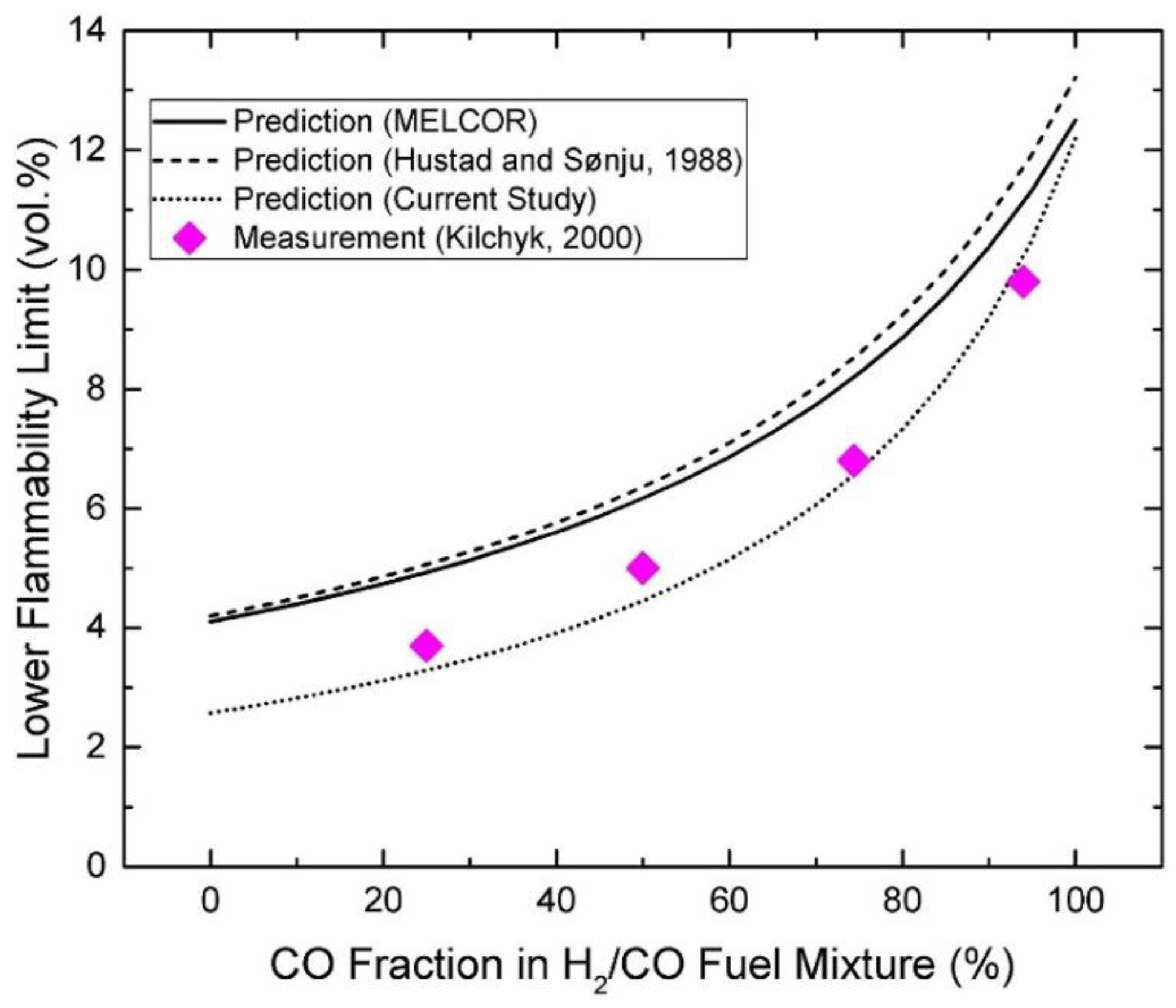
- Kilchyk, V. Flammability Limits of Carbon Monoxide and Carbon Monoxide-Hydrogen Mixtures in Air at Elevated Temperatures. Ph.D. Thesis, University of Calgary, Calgary, AB, Canada, 2000. [Google Scholar]
- Oostenrijk, B. Earth Gravity Flame Balls, or Are They? Master’s Thesis, Eindhoven University of Technology, Eindhoven, The Netherlands, 2012. [Google Scholar]
- Zel’dovich, Y.B. Teoriya Goreniya i Detonatsii Gazov (Theory of Combustion and Detonation of Gases); Akad, Nauk SSSR: Moscow, Russia, 1944. [Google Scholar]
- Ronney, P.D. Understanding combustion processes through microgravity research. Proc. Combust. Inst. 1998, 27, 2485–2506. [Google Scholar] [CrossRef]
- Ronney, P.D. Near-limit flame structures at low Lewis number. Combust. Flame 1990, 82, 1–14. [Google Scholar] [CrossRef]
- Ronney, P.D. Effect of gravity on laminar premixed gas combustion II: Ignition and extinction phenomena. Combust. Flame 1985, 62, 121–133. [Google Scholar] [CrossRef]
- Markstein, G.H. Nonsteady Flame Propagation; Pergamon Press: Oxford, UK, 1964. [Google Scholar]
- Bregeon, B.; Gordon, A.S.; Williams, F.A. Near-limit downward propagation of hydrogen and methane flames in oxygen-nitrogen mixtures. Combust. Flame 1978, 33, 33–45. [Google Scholar] [CrossRef]
- Liu, G.; Ye, Z.; Sohrab, S.H. On radiative cooling and temperature profiles of counterflow premixed flames. Combust. Flame 1986, 64, 193–201. [Google Scholar] [CrossRef]
- Ishizuka, S.; Law, C.K. An experimental study on extinction and stability of stretched premixed flames. Proc. Combust. Inst. 1982, 19, 327–335. [Google Scholar] [CrossRef]
- Sato, J. Effects of Lewis number on extinction behavior of premixed flames in a stagnation flow. Proc. Combust. Inst. 1982, 19, 1541–1548. [Google Scholar] [CrossRef]
- Tsuji, H.; Yamaoka, I. Structure and extinction of near-limit flames in a stagnation flow. Proc. Combust. Inst. 1982, 19, 1533–1540. [Google Scholar] [CrossRef]
- Sohrab, S.; Ye, Z.; Law, C.K. An experimental investigation on flame interaction and the existence of negative flame speeds. Proc. Combust. Inst. 1985, 20, 1957–1965. [Google Scholar] [CrossRef]
- Ju, Y.; Guo, H.; Maruta, K.; Liu, F. On the extinction limit and flammability limit of non-adiabatic stretched methane–air premixed flames. J. Fluid Mech. 1997, 342, 315–334. [Google Scholar] [CrossRef]
- Karlovitz, B.; Denniston, D.W., Jr.; Knapschaefer, D.H.; Wells, F. Studies on Turbulent flames: A. Flame Propagation Across velocity gradients B. turbulence Measurement in flames. Proc. Combust. Inst. 1953, 4, 613–620. [Google Scholar] [CrossRef]
- Matalon, M.; Cui, C.; Bechtold, J. Hydrodynamic theory of premixed flames: Effects of stoichiometry, variable transport coefficients and arbitrary reaction orders. J. Fluid Mech. 2003, 487, 179–210. [Google Scholar] [CrossRef]
- Platt, J.; Tien, J. Flammability of a Weakly Stretched Premixed Flame: The Effect of Radiation Loss; Fall Technical Meeting of the Eastern States Section of the Combustion Institute: Orlando, FL, USA, 1990. [Google Scholar]
- Tsuji, H. Thermal Engineering Joint Conference Proceedings. In Proceedings of the JSME-ASME Thermal Engineering Joint Conference, Honolulu, HI, USA, 20–24 March 1983. [Google Scholar]
- Guo, H.; Ju, Y.; Maruta, K.; Niioka, T.; Liu, F. Radiation extinction limit of counterflow premixed lean methane-air flames. Combust. Flame 1997, 109, 639–646. [Google Scholar] [CrossRef]
- Jarosinski, J.; Strehlow, R.; Azarbarzin, A. The mechanisms of lean limit extinguishment of an upward and downward propagating flame in a standard flammability tube. Proc. Combust. Inst. 1982, 19, 1549–1557. [Google Scholar] [CrossRef]
- Shoshin, Y.; Jarosinski, J. On extinction mechanism of lean limit methane–air flame in a standard flammability tube. Proc. Combust. Inst. 2009, 32, 1043–1050. [Google Scholar] [CrossRef]
- Fernández-Galisteo, D.; Sánchez, A.L.; Liñán, A.; Williams, F.A. One-step reduced kinetics for lean hydrogen–air deflagration. Combust. Flame 2009, 156, 985–996. [Google Scholar] [CrossRef]
- Bertolino, A.; Stagni, A.; Cuoci, A.; Faravelli, T.; Parente, A.; Frassoldati, A. Prediction of flammable range for pure fuels and mixtures using detailed kinetics. Combust. Flame 2019, 207, 120–133. [Google Scholar] [CrossRef]
- Saxena, P.; Williams, F.A. Testing a small detailed chemical-kinetic mechanism for the combustion of hydrogen and carbon monoxide. Combust. Flame 2006, 145, 316–323. [Google Scholar] [CrossRef]
- Lakshmisha, K.; Paul, P.; Mukunda, H. On the flammability limit and heat loss in flames with detailed chemistry. Proc. Combust. Inst. 1991, 23, 433–440. [Google Scholar] [CrossRef]
- Giovangigli, V.; Smooke, M. Application of continuation methods to plane premixed laminar flames. Combust. Sci. Technol. 1993, 87, 1993. [Google Scholar] [CrossRef]
- Ju, Y.; Masuya, G.; Ronney, P.D. Effects of radiative emission and absorption on the propagation and extinction of premixed gas flames. Proc. Combust. Inst. 1998, 27, 2619–2626. [Google Scholar] [CrossRef]
- Van den Schoor, F.; Verplaetsen, F.; Berghmans, J. Calculation of the upper flammability limit of methane/air mixtures at elevated pressures and temperatures. J. Hazard. Mater. 2008, 153, 1301–1307. [Google Scholar] [CrossRef] [PubMed]
- Shoshin, Y.; Tecce, L.; Jarosinski, J. Experimental and computational study of lean limit methane-air flame propagating upward in a 24 mm diameter tube. Combust. Sci. Technol. 2008, 180, 1812–1828. [Google Scholar] [CrossRef]
- Yakovenko, I.; Ivanov, M.; Kiverin, A.; Melnikova, K. Large-scale flame structures in ultra-lean hydrogen-air mixtures. Int. J. Hydrogen Energy 2018, 43, 1894–1901. [Google Scholar] [CrossRef]
- Jeon, J.; Jung, H.; Kim, Y.S.; Kim, S.J. Numerical study of lean limit hydrogen flames propagating upward to validate a flammability limit model. In Proceedings of the NURETH-18, Portland, OR, USA, 18–22 August 2019. [Google Scholar]
- Gerstein, M.; Stine, W.B. Analytical criteria for flammability limits. Proc. Combust. Inst. 1973, 14, 1109–1118. [Google Scholar] [CrossRef]
- Tsatsaronis, G. Prediction of propagating laminar flames in methane, oxygen, nitrogen mixtures. Combust. Flame 1978, 33, 217–239. [Google Scholar] [CrossRef]
- Warnatz, J. Rate Coefficients in the C/H/O System; Springer: New York, NY, USA, 1984. [Google Scholar]
- Giovangigli, V.; Smooke, M. Adaptive continuation algorithms with application to combustion problems. Appl. Numer. Math. 1989, 5, 305–331. [Google Scholar] [CrossRef]
- Lee, S.; Chung, D.; Chung, S. Local equilibrium temperature as a measure of stretch and preferential diffusion effects in counterflow H2/air premixed flames. Proc. Combust. Inst. 1998, 27, 579–585. [Google Scholar] [CrossRef]
- Dong, Y.; Holley, A.T.; Andac, M.G.; Egolfopoulos, F.N.; Davis, S.G.; Middha, P.; Wang, H. Extinction of premixed H2/air flames: Chemical kinetics and molecular diffusion effects. Combust. Flame 2005, 142, 374–387. [Google Scholar] [CrossRef]
- Wu, M.S.; Liu, J.B.; Ronney, P.D. Numerical simulation of diluent effects on flame balls. Proc. Combust. Inst. 1998, 27, 2543–2550. [Google Scholar] [CrossRef]
- Wu, M.S.; Ronney, P.D.; Colantonio, R.O.; VanZandt, D.M. Detailed numerical simulation of flame ball structure and dynamics. Combust. Flame 1999, 116, 387–397. [Google Scholar] [CrossRef]
- Seigel, R.; Howell, J.R. Thermal Radiation Heat Transfer; CRC Press: New York, NY, USA, 1981. [Google Scholar]
- Spalding, D. A theory of inflammability limits and flame-quenching. Proc. R. Soc. Lond. A 1957, 240, 83–100. [Google Scholar]
- Kee, R.J.; Miller, J.A.; Evans, G.H.; Dixon-Lewis, G. A computational model of the structure and extinction of strained, opposed flow, premixed methane-air flames. Proc. Combust. Inst. 1989, 22, 1479–1494. [Google Scholar] [CrossRef]
- Giovangigli, V.; Smooke, M. Extinction of strained premixed laminar flames with complex chemistry. Combust. Sci. Technol. 1987, 53, 23–49. [Google Scholar] [CrossRef]
- Egerton, A.C. Limits of inflammability. Proc. Combust. Inst. 1953, 4, 4–13. [Google Scholar] [CrossRef]
- Zabetakis, M.G. Flammability Characteristics of Combustible Gases and Vapors; Bureau of Mines: Washington, DC, USA, 1965.
- MAČEK, A. Flammability limits: A re-examination. Combust. Sci. Technol. 1979, 21, 43–52. [Google Scholar] [CrossRef]
- Cheng, T.K.H. An Experimental Study of the Rich Flammability Limits of Some Gaseous Fuels and Their Mixtures in Air. Master’s Thesis, University of Calgary, Calgary, AB, Canada, 1985. [Google Scholar]
- Hansen, T.J.; Crowl, D.A. Estimation of the flammability zone boundaries for flammable gases. Process Saf. Prog. 2010, 29, 209–215. [Google Scholar] [CrossRef]
- Bade Shrestha, S.O. Systematic Approach to Calculations of Flammability Limits of Fuel-Diluent Mixtures in Air. Master’s Thesis, University of Calgary, Calgary, AB, Canada, 1993. [Google Scholar]
- Mashuga, C.V.; Crowl, D.A. Flammability zone prediction using calculated adiabatic flame temperatures. Process Saf. Prog. 1999, 18, 127–134. [Google Scholar] [CrossRef]
- Razus, D.; Molnarne, M.; Fuß, O. Limiting oxygen concentration evaluation in flammable gaseous mixtures by means of calculated adiabatic flame temperatures. Chem. Eng. Process. 2004, 43, 775–784. [Google Scholar] [CrossRef]
- Wan, X.; Zhang, Q.; Shen, S.L. Theoretical estimation of the lower flammability limit of fuel-air mixtures at elevated temperatures and pressures. J. Loss Prevent. Process Ind. 2015, 36, 13–19. [Google Scholar] [CrossRef]
- White, A.G. Limits for the propagation of flame in inflammable gas–air mixtures. Part III. The effects of temperature on the limits. J. Chem. Soc. 1925, 127, 672–684. [Google Scholar] [CrossRef]
- Lewis, B.; Von Elbe, G. Combustion, Flames and Explosions of Gases; Combustion and Explosives Researches, Inc.: Pittsburg, PA, USA, 2012. [Google Scholar]
- Bartok, W.; Sarofim, A.F. Fossil Fuel Combustion: A Source Book; Wiley: New York, NY, USA, 1991. [Google Scholar]
- Vidal, M.; Wong, W.; Rogers, W.; Mannan, M.S. Evaluation of lower flammability limits of fuel–air–diluent mixtures using calculated adiabatic flame temperatures. J. Hazard. Mater. 2006, 130, 21–27. [Google Scholar] [CrossRef] [PubMed]
- Melhem, G. A detailed method for estimating mixture flammability limits using chemical equilibrium. Process Saf. Prog. 1997, 16, 203–218. [Google Scholar] [CrossRef]
- Burgess, D.; Hertzberg, M. The flammability limits of lean fuel-air mixtures: Thermochemical and kinetic criteria for explosion hazards. ISA Trans. 1975, 14, 129–136. [Google Scholar] [PubMed]
- Britton, L.G. Using heats of oxidation to evaluate flammability hazards. Process Saf. Prog. 2002, 21, 31–54. [Google Scholar] [CrossRef]
- Vidal, M.; Rogers, W.; Holste, J.; Mannan, M.S. A review of estimation methods for flash points and flammability limits. Process Saf. Prog. 2004, 23, 47–55. [Google Scholar] [CrossRef]
- Ma, T. A thermal theory for estimating the flammability limits of a mixture. Fire Saf. J. 2011, 46, 558–567. [Google Scholar] [CrossRef]
- Lovachev, L.; Kaganova, Z. Calculation of hydrogen bromide flame characteristics. Dokl. Akad. Nauk SSSR 1969, 188, 1087. [Google Scholar]
- Lovachev, L. The theory of limits on flame propagation in gases. Combust. Flame 1971, 17, 275–278. [Google Scholar] [CrossRef]
- Ural, E.A.; Zalosh, R.G. A mathematical model for lean hydrogen-air-steam mixture combustion in closed vessels. Proc. Combust. Inst. 1985, 20, 1727–1734. [Google Scholar] [CrossRef]
- Frank-Kamenetskii, D.A. Diffusion and Heat Transfer in Chemical Kinetics; Princeton University Press: Princeton, NJ, USA, 1969. [Google Scholar]
- Liu, D.; MacFarlane, R. Laminar burning velocities of hydrogen-air and hydrogen-air steam flames. Combust. Flame 1983, 49, 59–71. [Google Scholar] [CrossRef]
- Crescitelli, S.; Russo, G.; Tufano, V. Flame propagation in closed vessels and flammability limits. Combust. Sci. Technol. 1977, 15, 201–212. [Google Scholar] [CrossRef]
- Fenn, J.B.; Calcote, H.F. Activation energies in high temperature combustion. Proc. Combust. Inst. 1953, 4, 231–239. [Google Scholar] [CrossRef]
- Morales, G.F.; Ehrhart, B.D.; Muna, A.B. HyRAM (Hydrogen Risk Assessment Models), Version 2.0 User Guide; Sandia National Laboratories: Albuquerque, NM, USA, 2019.
- Nishimura, T.; Hoshi, H.; Hotta, A. Current research and development activities on fission products and hydrogen risk after the accident at Fukushima Daiichi nuclear power station. Nucl. Eng. Technol. 2015, 47, 1–10. [Google Scholar] [CrossRef]
- Liaw, H.J.; Chen, K.Y. A model for predicting temperature effect on flammability limits. Fuel 2016, 178, 179–187. [Google Scholar] [CrossRef]
- Matsukov, I.; Kunetzov, M.; Alekseev, V.; Dorofeev, S. Photographic Study of the Characteristic Regimes of Turbulent Flame Propagation, Local and Global Quenching in Obstructed Areas; FZK-INR: Moscow, Russia, 1998. [Google Scholar]
- Joulin, G.; Clavin, P. Linear stability analysis of nonadiabatic flames: Diffusional-thermal model. Combust. Flame 1979, 35, 139–153. [Google Scholar] [CrossRef]
- Clavin, P.; Williams, F.A. Effects of molecular diffusion and of thermal expansion on the structure and dynamics of premixed flames in turbulent flows of large scale and low intensity. J. Fluid Mech. 1982, 116, 251–282. [Google Scholar] [CrossRef]
- Strehlow, R.A.; Noe, K.A.; Wherley, B.L. The effect of gravity on premixed flame propagation and extinction in a vertical standard flammability tube. Proc. Combust. Inst. 1988, 21, 1899–1908. [Google Scholar] [CrossRef]


| Authors | Dimension of Tube (cm) | Observed Limit (vol%) | Ref. | ||
|---|---|---|---|---|---|
| Diameter | Length | LFL | UFL | ||
| White | 7.5 | 150 | 4.2 | 75.0 | [25] |
| Egerton et al. | 5.3 | 150 | 4.2 | 74.6 | [26] |
| Egerton et al. | 5.3 | 150 | 4.1 | 74.3 | [26] |
| Egerton et al. | 5.3 | 150 | 4.2 | 74.8 | [26] |
| White | 5.0 | 150 | 4.2 | 74.5 | [25] |
| Jones | 5.0 | 180 | 4.0 | 72.0 | [27] |
| Burgoyne et al. | 4.8 | 150 | 4.0 | 73.8 | [28] |
| Clusius et al. | 4.5 | 80 | 4.1 | - | [29] |
| Payman | 2.5 | 150 | 4.2 | - | [30] |
| White | 2.5 | 150 | 4.3 | 73.0 | [25] |
| Method | Bureau of Mines (Coward and Jones) | DIN 51 649 | EN 1839 Tube |
|---|---|---|---|
| Tube geometry | Open tube D = 5 cm, L = 1.5 m | Open tube D = 6 cm, L = 0.3 m | Open tube D = 8 cm, L = 0.3 m |
| Ignition source | spark/flame bottom end | spark bottom end E = 5 J, t = 0.5 s | spark bottom end E = 2 J, t = 0.2 s |
| Flammability criterion | visual flame propagation over 1.5 m | visual flame detachment | visual flame propagation over 0.1 m |
| Flammability limit definition | halfway between the flammable and non-flammable point | at non-flammable point | at non-flammable point |
| Year | Authors | Mixture | Tube Geometry | Ref. |
|---|---|---|---|---|
| 1957 | Scott et al. | H2-NO-N2O H2-N2O-air H2-NO-air | Bureau of Mines | [32] |
| 1984 | Shebeko et al. | H2-O2-He H2-O2-CO2 H2-O2-N2 H2-O2-Ar | - | [33] |
| 1985 | Kumar | H2-O2-N2 H2-O2-CO2 H2-O2-H2O H2-Air-H2O H2-O2-Ar H2-O2-He | Bureau of Mines | [34] |
| 1986 | Marshall | H2-air-H2O | FITS vessel | [35] |
| 1988 | Hustad et al. (b) | H2-air | D = 10 cm, L = 3 m | [36] |
| 1995 | Shebeko (a) | H2-O2-He H2-O2-CO2 H2-O2-N2 H2-O2-Ar H2-O2-He-H2O H2-O2-He-CO2 H2-O2-N2-CO2 | D = 30 cm, L = 80 cm | [37] |
| 1998 | Ale (c) | H2-air | Bureau of Mines | [38] |
| 2001 | Wierzba et al. | H2-CO-air | Bureau of Mines | [7] |
| 2007 | Van den Schoor (d) | H2-CH4-air | DIN 51 649 | [31] |
| 2012 | Terpstra | H2-air H2-air-N2 H2-air-He H2-air-Ar H2-air-CO2 | Bureau of Mines | [15] |
| 2014 | Liu et al. (e) | H2-air | D = 16 cm, L = 0.34 m | [39] |
| 2015 | Hernandez-Perez et al. (f) | H2-CH4-air | D = 1.35 cm, L = 3 cm | [18] |
| 2018 | Zhou et al. (f) | H2-air H2-CH4-air | D = 1.35 cm, L = 10 cm | [22] |
| 2020 | Xu et al. | H2-O2-N2 H2-O2-CO2 | D = 18 cm, L = 20 cm | [40] |
| Researcher | Mixture | Ref. |
|---|---|---|
| Kilchyk | H2-CO-air | [57] |
| H2-CO-air | ||
| H2-CO-air | ||
| H2-CO-air-H2O | ||
| H2-CO-air-H2O | ||
| Wang et al. | H2-CO-O2-N2 | [55] |
| H2-CO-O2-N2 | ||
| Grune et al. | H2-CO-O2-N2-H2O-CO2 | [56] |
| H2-CO-O2-N2-H2O-CO2 |
| Type | Reaction |
|---|---|
| Shuffle reactions | |
| Hydroperoxyl reactions | |
| Radical-radical recombination reactions | |
| Hydrogen peroxide reactions | |
| Year | Researcher | Numerical Method | Mixture | Ref. |
|---|---|---|---|---|
| 1990 | Lakshmisha et al. | 1D/planar/non-adiabatic/unsteady | CH4-air | [81] |
| 1992 | Giovangigli et al. | 1D/planar/adiabatic/unsteady | H2-air CH4-air | [82] |
| 1992 | Law et al. | 1D/planar/non-adiabatic/steady | H2-air CH4-air | [43] |
| 1998 | Ju et al. | 1D/planar/non-adiabatic/steady | CH4-air | [83] |
| 2008 | Van den Schoor et al. | 1D/planar and spherical/non-adiabatic/steady and unsteady | CH4-air | [84] |
| 2008 | Shoshin et al. | 2D/stretched/non-adiabatic/unsteady | CH4-air | [85] |
| 2009 | Fernandez-Galisteo et al. | 1D/planar/adiabatic/steady/7step | H2-air | [21] |
| 2015 | Hernandez-Perez et al. | 2D/stretched/non-adiabatic/steady | H2-CH4-air | [18] |
| 2018 | Zhou et al. | 2D/stretched/non-adiabatic/steady | H2-CH4-air | [16] |
| 2018 | Zhou et al. | 2D/stretched/non-adiabatic/steady | H2-air CH4-air H2-CH4-air | [22] |
| 2018 | Yakovenko et al. | 2D/stretched/non-adiabatic/unsteady | H2-air | [86] |
| 2019 | Bertolino et al. | 1D/planar/non-adiabatic/steady | CH4-air CH3OH-air C2H6-air C3H8-air, etc. | [79] |
| 2019 | Jeon et al. | 2D/stretched/non-adiabatic/unsteady | H2-air | [87] |
| Fuel | Exp. | Num. (2D) | 1D Flat Flame | 1D Flame Ball |
|---|---|---|---|---|
| CH4 | 0.480 | 0.445 | 0.497 | - |
| 40%H2 + 60%CH4 | 0.350 | 0.315 | 0.446 | 0.270 |
| H2 | 0.090 | 0.110 | 0.295 | 0.073 |
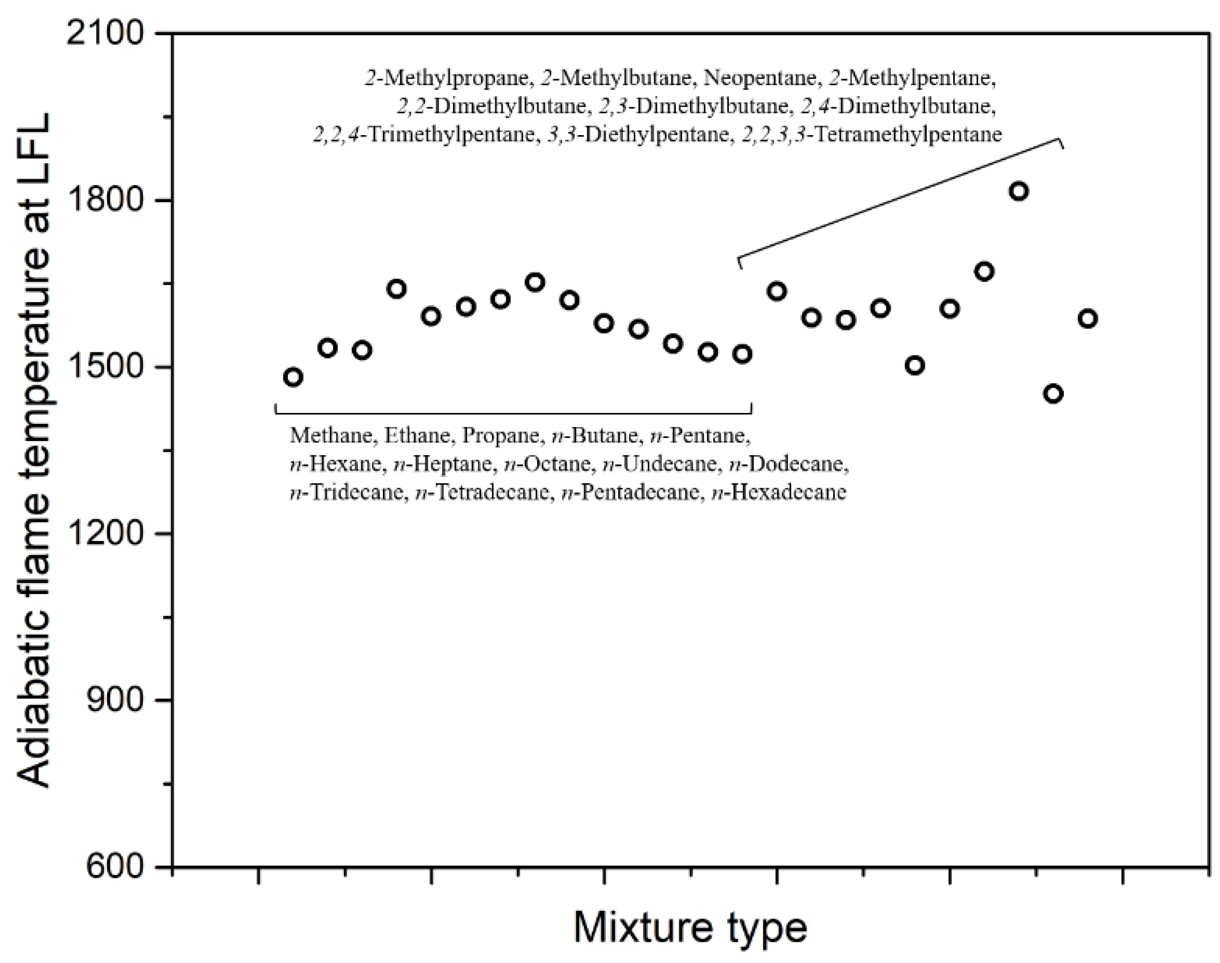
| Fuel | LFL | |
|---|---|---|
| CH4 | 5.0 | 1480 |
| C2H6 | 3.0 | 1530 |
| C3H8 | 2.1 | 1540 |
| n-C4H10 | 1.8 | 1640 |
| n-C5H12 | 1.4 | 1590 |
| n-C6H14 | 1.2 | 1610 |
| n-C7H16 | 1.0 | 1620 |
| n-C8H18 | 0.9 | 1650 |
| Pressure (bar) | 298 K | 473 K | |
|---|---|---|---|
| 1 | 1692 | 1678 | 1667 |
| 3 | 1648 | 1622 | 1612 |
| 6 | 1597 | 1583 | 1584 |
| 10 | 1545 | 1533 | 1524 |
| Researcher | Mixture | (°C) | Diluent (vol%) | LFL (vol%) | CAFT (K) | Ref. |
|---|---|---|---|---|---|---|
| Terpstra | H2-air | 20 | 0 | 3.9 | 610 | [15] |
| H2-air | 50 | 0 | 3.8 | 633 | ||
| H2-air | 100 | 0 | 3.6 | 667 | ||
| H2-air | 150 | 0 | 3.3 | 692 | ||
| H2-air | 200 | 0 | 2.8 | 701 | ||
| H2-air | 300 | 0 | 2.4 | 769 | ||
| H2-air-He | 20 | 0–50 | 3.8–5.3 | 600–800 | ||
| H2-air-Ar | 20 | 0–60 | 3.0–3.8 | 590–610 | ||
| H2-air-N2 | 20 | 0–20 | ~3.9 | ~610 | ||
| H2-air-CO2 | 20 | 0–40 | 3.9–4.6 | 602~620 | ||
| Kumar | H2-O2-He | 22 | 20–40 | 5.1–5.8 | 700–800 | [34] |
| H2-O2-He | 100 | 20–40 | 3.9–4.3 | 700–750 | ||
| H2-O2-N2 | 22 | 20–40 | ~4.0 | ~600 | ||
| H2-O2-N2 | 100 | 20–40 | ~3.5 | ~650 | ||
| Hustad | H2-air | 20 | 0 | 4.3 | 644 | [36] |
| H2-air | 200 | 0 | 3.3 | 741 | ||
| Marshall | H2-air-Steam | 100–120 | 10 | 4.83 | 773 | [35] |
| H2-air-Steam | 100–120 | 20 | 5.31 | 804 | ||
| H2-air-Steam | 100–120 | 30 | 5.96 | 847 | ||
| H2-air-Steam | 100–120 | 40 | 6.93 | 913 |
Publisher’s Note: MDPI stays neutral with regard to jurisdictional claims in published maps and institutional affiliations. |
© 2020 by the authors. Licensee MDPI, Basel, Switzerland. This article is an open access article distributed under the terms and conditions of the Creative Commons Attribution (CC BY) license (http://creativecommons.org/licenses/by/4.0/).
Share and Cite
Jeon, J.; Kim, S.J. Recent Progress in Hydrogen Flammability Prediction for the Safe Energy Systems. Energies 2020, 13, 6263. https://doi.org/10.3390/en13236263
Jeon J, Kim SJ. Recent Progress in Hydrogen Flammability Prediction for the Safe Energy Systems. Energies. 2020; 13(23):6263. https://doi.org/10.3390/en13236263
Chicago/Turabian StyleJeon, Joongoo, and Sung Joong Kim. 2020. "Recent Progress in Hydrogen Flammability Prediction for the Safe Energy Systems" Energies 13, no. 23: 6263. https://doi.org/10.3390/en13236263
APA StyleJeon, J., & Kim, S. J. (2020). Recent Progress in Hydrogen Flammability Prediction for the Safe Energy Systems. Energies, 13(23), 6263. https://doi.org/10.3390/en13236263