A Hybrid System Based on LSTM for Short-Term Power Load Forecasting


Abstract
1. Introduction
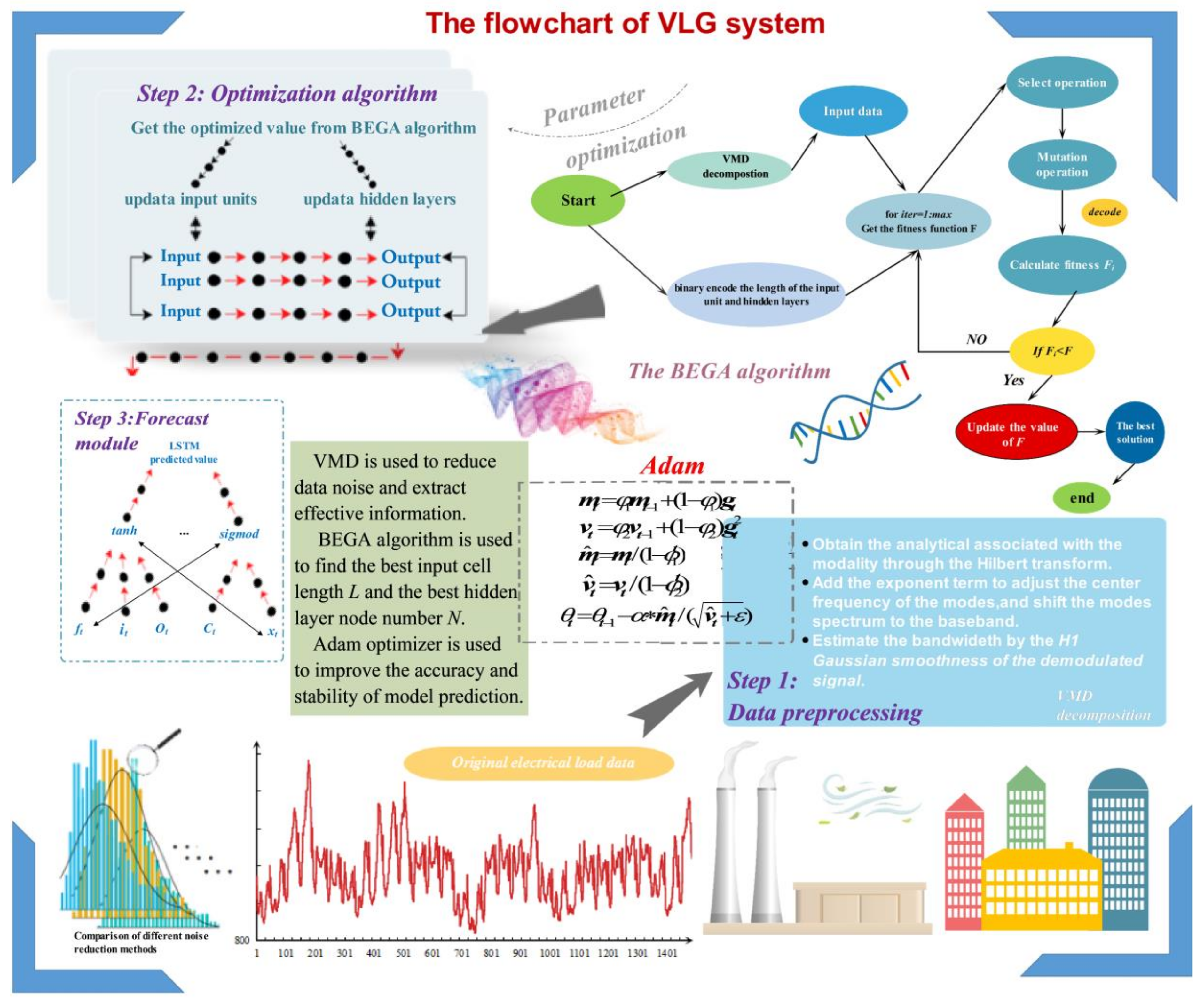
- The original power load data is decomposed and reconstructed using VMD technology to extract the effective features of the data. This reduces the adverse effects of the instability and irregularity of the original load data on the forecasting model.
- The long-term and short-term memory neural network is applied to forecast the power load data. This solves the problem where the time series depends on previous data and overcomes the low accuracy and poor stability of traditional models.
- A binary encoding genetic algorithm is proposed to adaptively decide the hidden layer nodes and the length of the input data unit of the LSTM. This algorithm abandons the traditional decimal coding method and uses binary coding for integer optimization.
- The adaptive moment estimation (Adam) algorithm is employed for optimizing the model’s hyperparameters, instead of the traditional gradient descent algorithm and stochastic gradient descent algorithm (SGD). This improves the convergence speed and prediction stability of the model.
- The prediction model optimized by the hybrid optimization method has high prediction accuracy and good stability, thereby effectively improving the accuracy of power load prediction.
2. Related Theory
2.1. Variational Mode Decomposition (VMD)
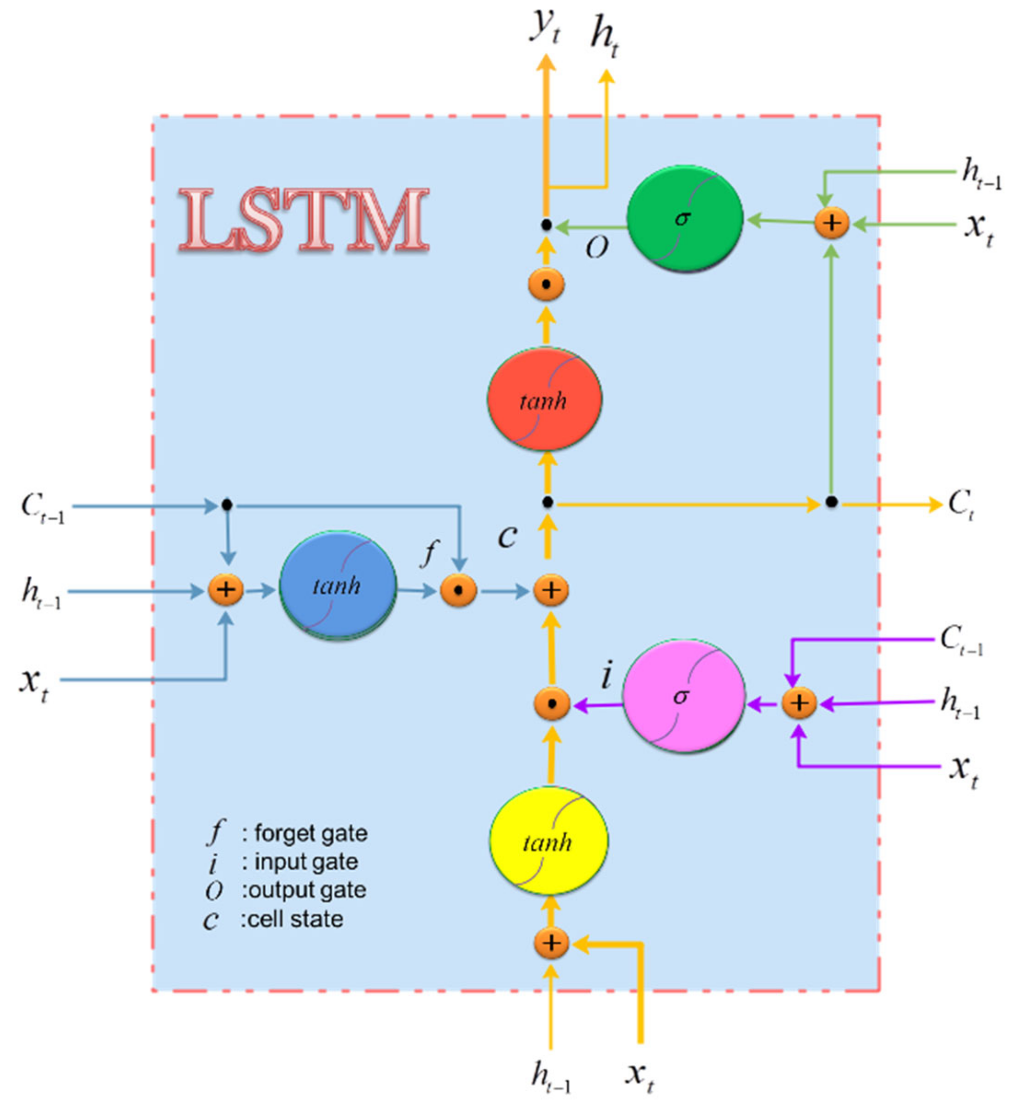
2.2. Long Short Term Memory Neural Network (LSTM)
2.3. Binary Encoding Genetic Algorithm (BEGA)
2.4. Adaptive Moment Estimation Optimizer (Adam)
3. The Formation of the Combined Forecasting System
3.1. Data Preprocessing Module
3.2. Optimization Algorithm Module
3.3. Forecast Module
4. Experiment and Evaluation
4.1. Model Evaluation Indicators
4.2. Experimental Setup
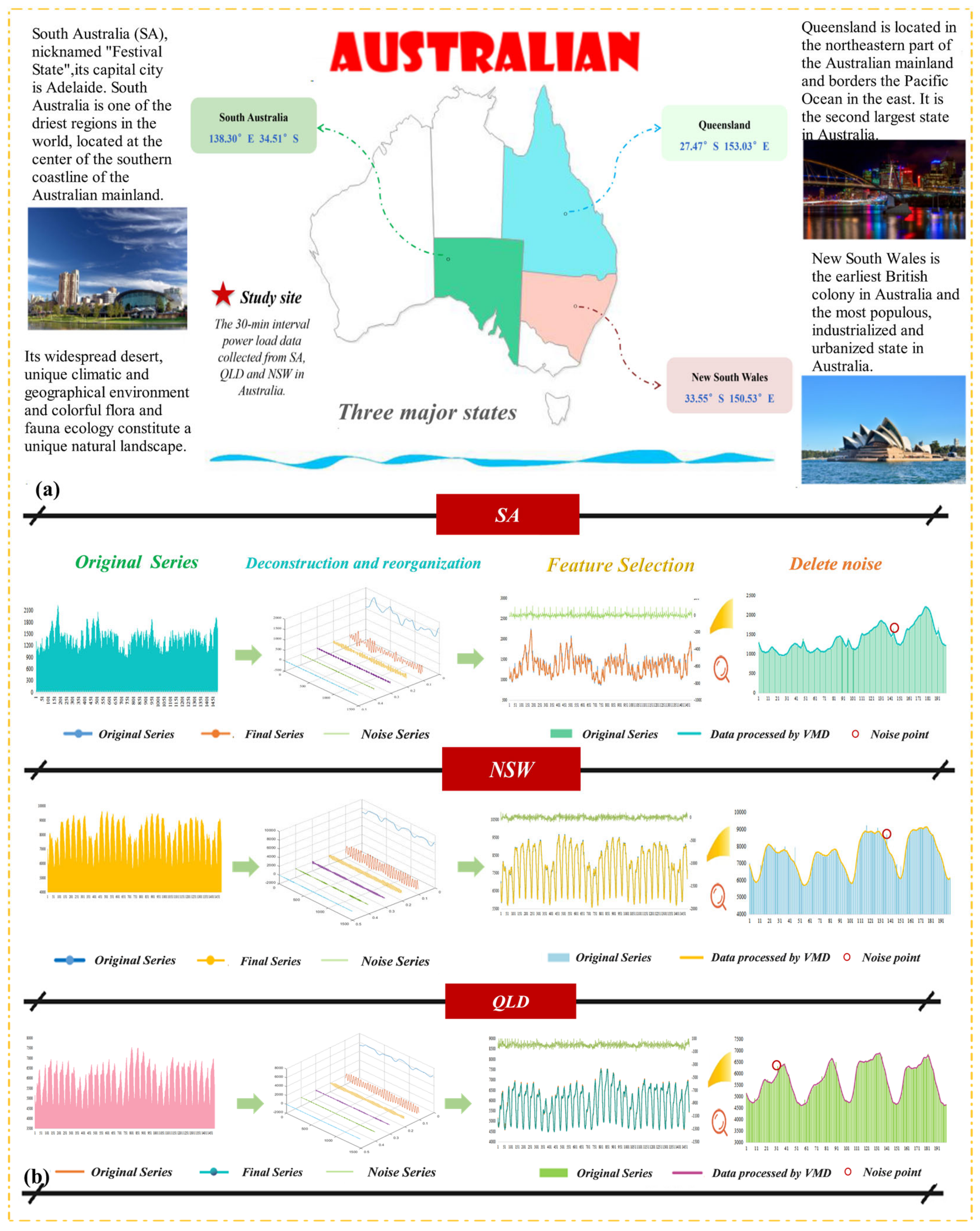
4.3. Data Description
4.4. Model Parameter Setting
4.4.1. Parameter Setting of the ANN
4.4.2. Parameter Settings of the Optimization Algorithm
4.5. Experiment I
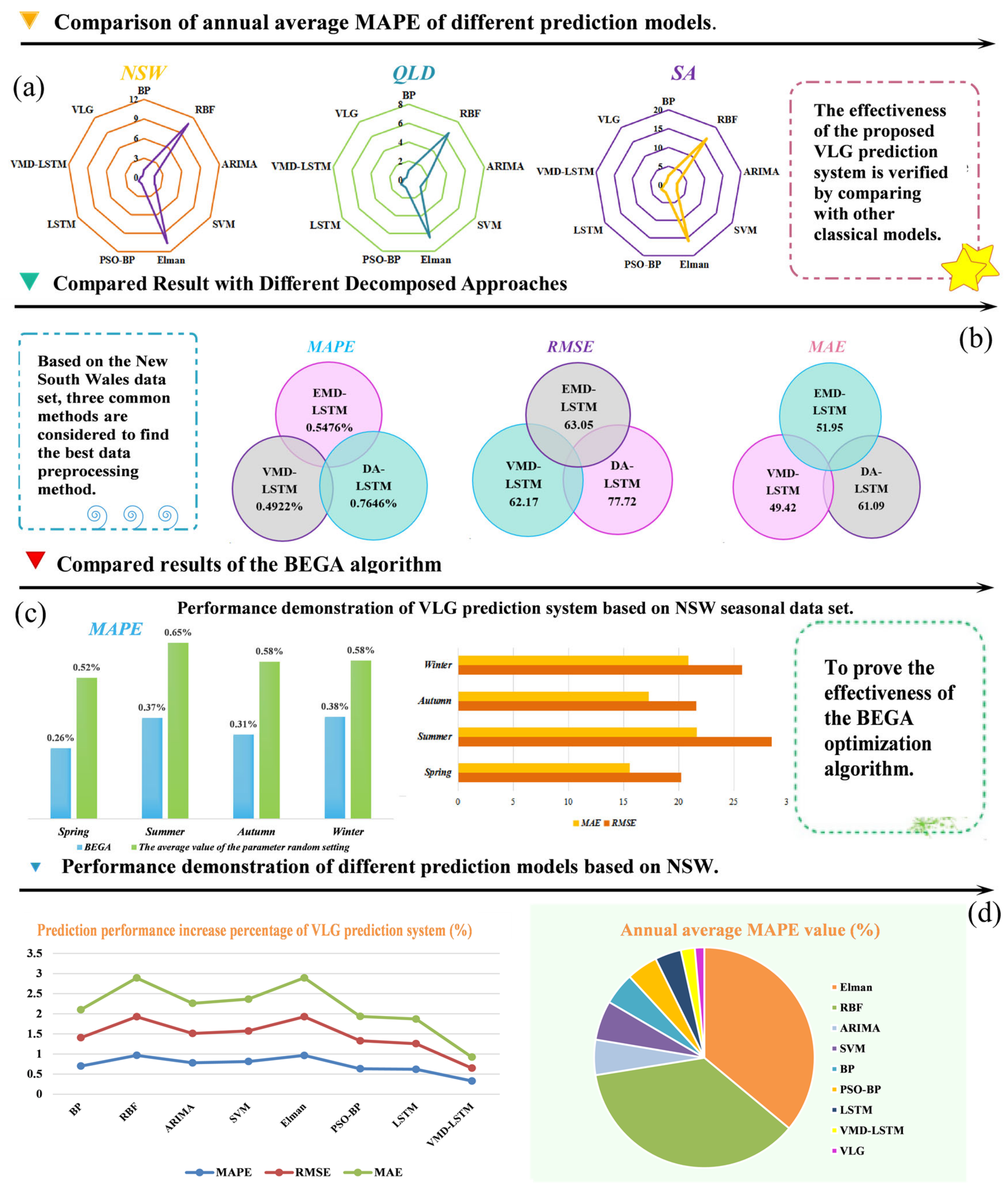
- (a)
- The comparison results of the evaluation index system of VMD-LSTM and other hybrid systems are introduced in this table. The VMD-LSTM shows better prediction accuracy and prediction performance on most evaluation indicators. For the comparison between the single LSTM model and the VMD-LSTM system, it is obvious that the evaluation index of the VMD-LSTM system is superior to that of the LSTM model in all cases. At the same time, the prediction accuracy of all noise reduction models is higher than that of the model based on original data, which indicates that data preprocessing is indispensable for power load prediction.
- (b)
- In the case, we compare the VMD-LSTM model and several other hybrid model methods. Among the performance test index values of the experiments in various regions, the VMD-LSTM model offers the best MAPE results, with 0.4859%, 0.9352%, and 0.4922%. Secondly, the models based on prediction accuracy are VMD-LSTM, EMD-LSTM, EMD-BP, VMD-BP, DA-LSTM, and DA-BP, in order from high to low. Among the six models, VMD-LSTM has the best prediction accuracy. The coefficient of determination (R2) reflects the difference in the performance of the prediction model from the fit. In this experiment, the R2 of VMD-LSTM is the best with 0.9971, 0.9910, and 0.9967 in the three states. We also certify the effectiveness of the noise reduction model VMD employed in this paper.
- (c)
- The previous time-series data denoising technology is also applied to the power load, short-term wind speed, and stock prediction models. Most of these models only discuss the improvement of model accuracy and performance via noise reduction technology but do not discuss the new sequence obtained after using the noise reduction method correlation with the original time series. Therefore, through the gray correlation method (GC) and the method of calculating the Pearson correlation coefficient (PE) and Spearman correlation coefficient (SP), the differences between different noise reduction methods are discussed from the perspective of the correlation between the new sequence and the original sequence. Detailed calculation results are given in Table 7.
4.6. Experiment II
4.7. Experiment III
5. Discussion
5.1. Effectiveness of the Proposed System
- (1)
- By contrasting and dissecting the forecasting errors of different hybrid systems, the DM test consequences of different prediction models are all at the upper limit at a confidence level of 1%;
- (2)
- The Diebold-Mariano test was performed on the prediction errors of four different traditional single models, and the test results of the VLG were all higher than the upper limit at a confidence level of 1%;
- (3)
- The minimum value of the comparison between the VLG combination system and the LSTM model using other data preprocessing technologies is 2.0104, which is also far beyond the 5% significance level threshold.
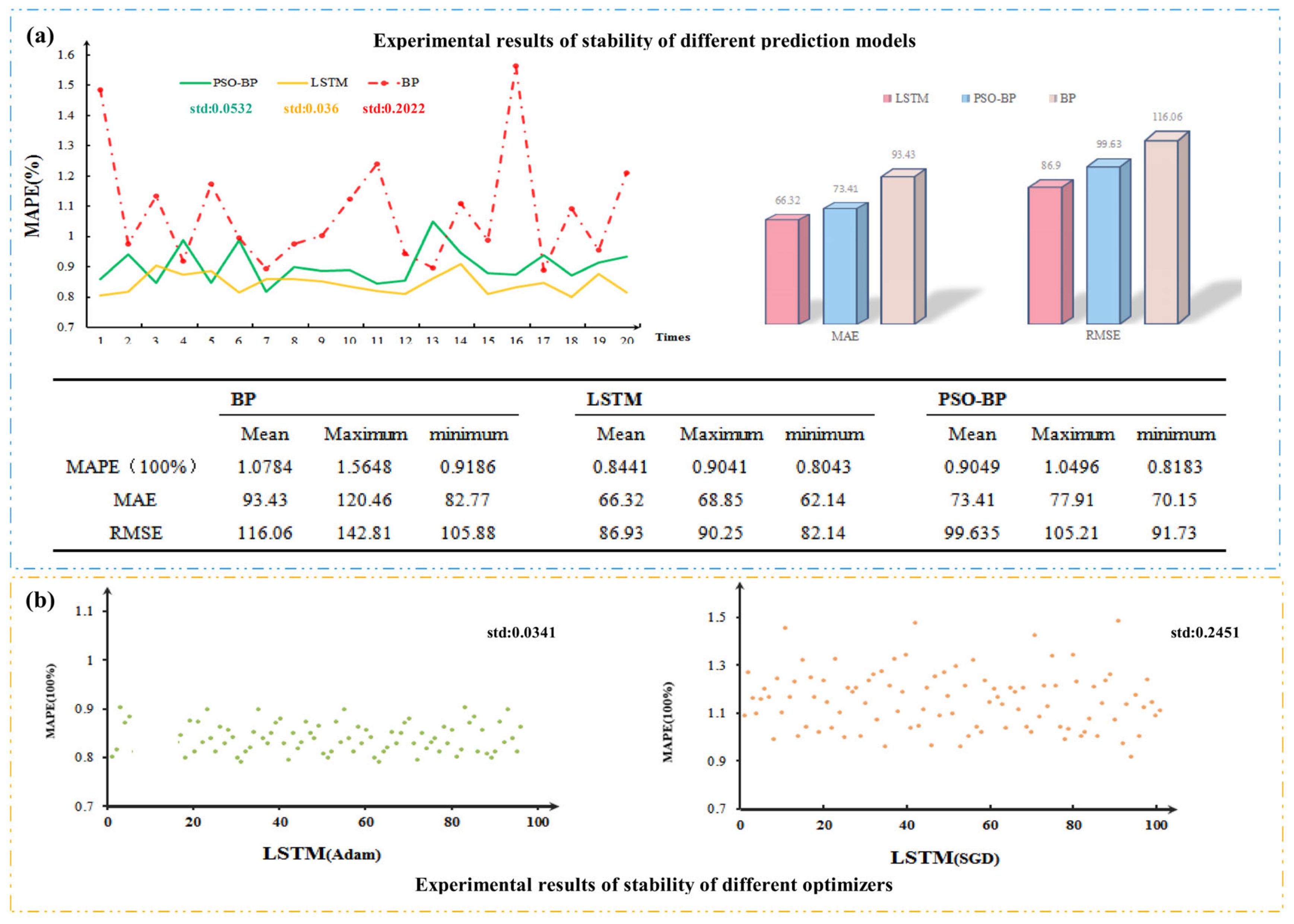
5.2. Model Stability Study
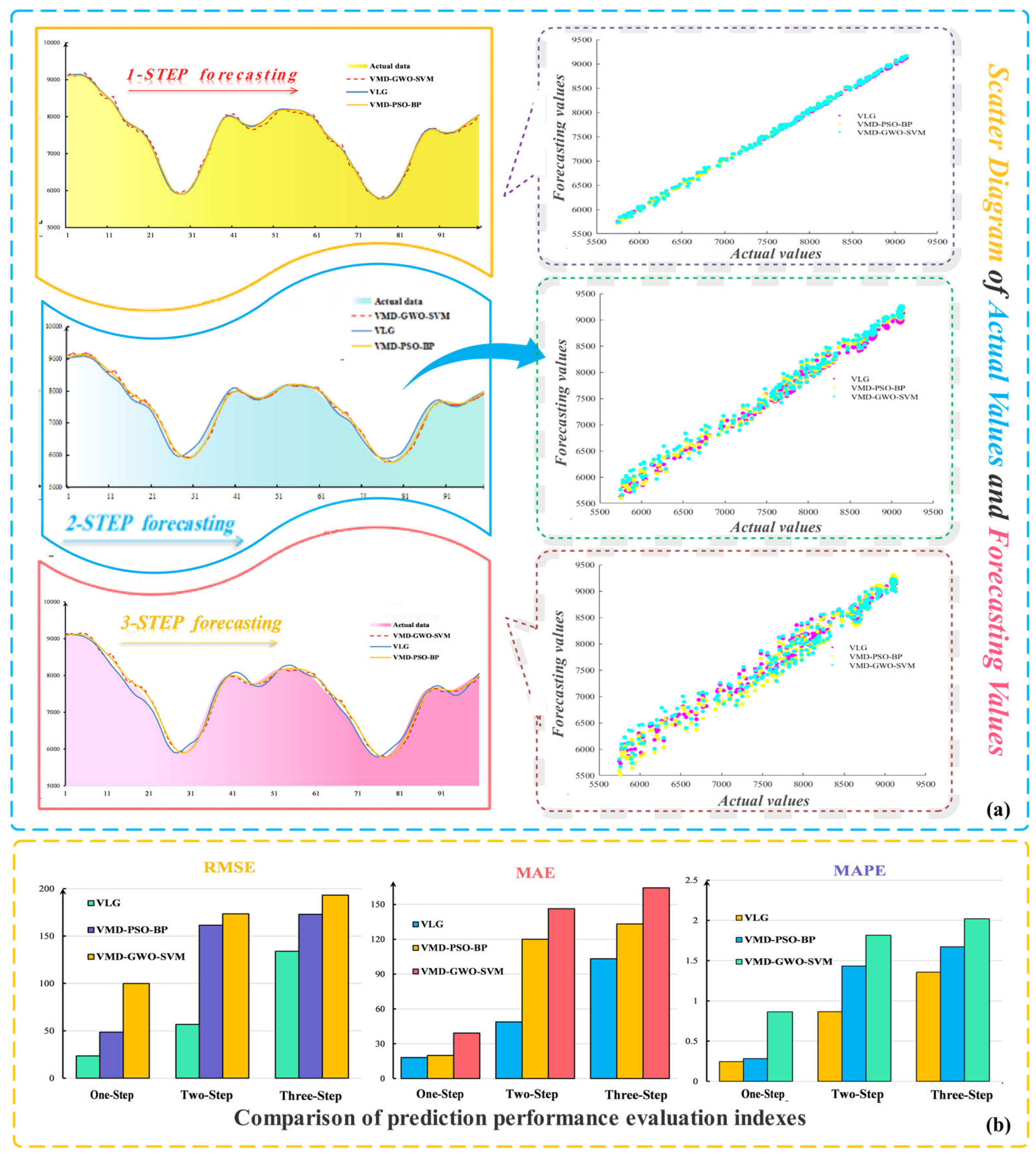
5.3. Multi-Step Prediction and Result Analysis
5.4. Improvement of the Evaluation Index
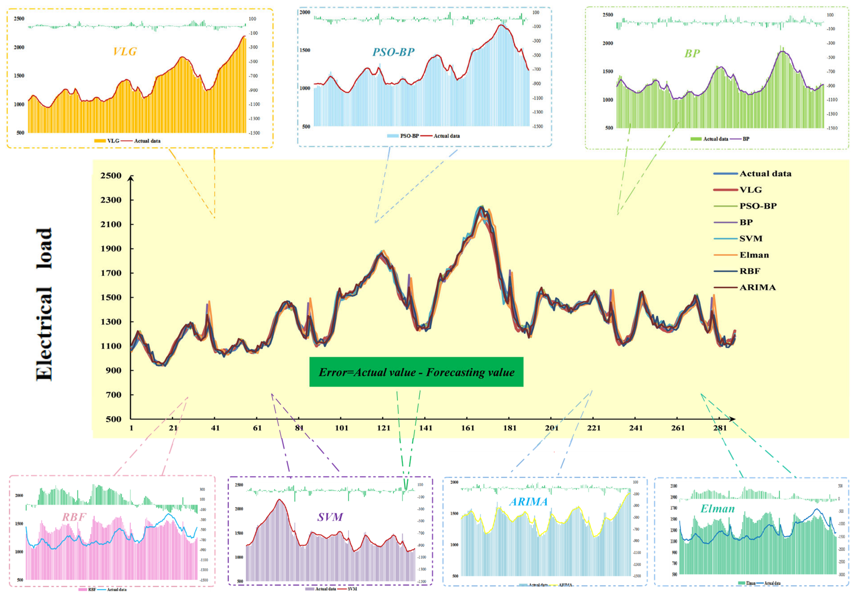
- (a)
- The predictive capacity of the system employed in this study is clearly commendable.
- (b)
- The value of the percentage improvement of the evaluation index shows a clear decreasing trend. This indicates that the prediction veracity of the system is gradually improved due to the data preprocessing technology and simulation optimization algorithm playing a vital role in improving the prediction ability of the system.
- (c)
- Notably, the VLG hybrid system presents obvious advantages over other systems.
5.5. Future and Prospects
6. Conclusions
Author Contributions
Funding
Acknowledgments
Conflicts of Interest
Abbreviations
| List of terminologies (method and indices) | |||
| EMD | Empirical model decomposition | DA | Denoise autoencoder |
| VMD | Variational Modal Decomposition | BP | Back propagation neural network |
| LSTM | Long Short-Term Memory neural network | RBF | Radial basis function |
| Elman | Elman neural network | SVM | Support vector machine |
| ARMA | Autoregressive moving average model | ARIMA | Autoregressive interval moving average model |
| PSO | Partial swarm optimization algorithm | GWO | Grey wolf optimization algorithm |
| EMD-BP | BP after EMD technology | DA-BP | BP after DA technology |
| VMD-BP | BP after VMD technology | EMD-LSTM | LSTM after EMD technology |
| DA-LSTM | LSTM after DA technology | VMD-LSTM | LSTM after VMD technology |
| GC | Grey correlation method | IMFs | Intrinsic mode functions |
| SP | Spearman correlation coefficient | PE | Pearson correlation coefficient |
| MAPE | Mean absolute percentage error | MAE | Mean absolute error |
| RMSE | Root Mean Square Error | R2 | Coefficient of determination |
| AI | Artificial intelligence | PSO-BP | BP after PSO optimization algorithm |
| Adam | Adaptive moment estimation optimization | SGD | Stochastic Gradient Descent |
| BEGA | Binary encoding genetic algorithm | EMD-LSTM GA | LSTM after EMD and GA optimization |
| DA-LSTM-GA | LSTM after DA and GA optimization | VMD-PSO-BP | BP after PSO and VMD optimization |
| VMD-GWO-SVM | VMD after VMD and GWO optimization | DM | Diebold-Mariano test |
| DL | Deep learning | RNN | Recurrent neural networks |
| CNN | Convolution neural network | BiLSTM | Bi-directional long-term memory neural network |
| ANNs | Artificial neural networks | PMAPE | The improvement in MAPE values |
| ADMM | Alternate Direction Method of Multipliers | VLG | The model combined VMD-BEGA -LSTM |
| List of terminologies (parameters and variables) | |||
| ωk | Center pulse frequency | N1 | Population Size of the GA |
| f | Actual signal | α | Initial learning rate |
| λ | Lagrange factor | xt | Corresponding input |
| uk(ω) | Modal function of VMD Technology | L1 | Binary encoding length |
| ft | Forget gate | it | Input gate |
| Ot | Output gate | Ct | Memory cell state |
| ht | T-1 time input | sigmoid | Input gate layer |
| Wf | Coefficient matrix | bf | Bias vector |
| gt | T gradient of time step | mt | Gradient mean |
| vt | Exponential moving average | β | Exponential decay rate |
| pi | Selection probability in genetic | xbin | Binary code |
| xdec | Decimal code | L | Input unit length |
| N | Number of cells in the hidden layer | loss | Loss function value of training model |
| ym | True value of data | The value of model forecast | |
| iter | Model iterations | y | Average of sequence data |
| ωk | Center pulse frequency | N1 | Population Size of the GA |
| f | Actual signal | xt | Corresponding input |
| The main terminologies mentioned in this paper (including indices, methods, variables and parameters). | |||
References
- Yang, W.; Wang, J.; Tong, N. A hybrid forecasting system based on a dual decomposition strategy and multi-objective optimization for electricity price forecasting. Appl. Energy 2019, 235, 1205–1225. [Google Scholar] [CrossRef]
- Guo, Z.; Zhou, K.; Zhang, X.; Yang, S. A deep learning model for short-term power load and probability density forecasting. Energy 2018, 160, 1186–1200. [Google Scholar] [CrossRef]
- Zhang, X.; Wang, J. A novel decomposition-ensemble model for forecasting short-term load-time series with multiple seasonal patterns. Appl. Soft Comput. 2018, 65, 478–494. [Google Scholar] [CrossRef]
- Wang, R.; Wang, J.; Xu, Y. A novel combined model based on hybrid optimization algorithm for electrical load forecasting. Appl. Soft Comput. 2019, 82, 105548. [Google Scholar] [CrossRef]
- He, Q.; Wang, J.; Lu, H. A hybrid system for short-term wind speed forecasting. Appl. Energy 2018, 226, 756–771. [Google Scholar] [CrossRef]
- Zhao, H.; Han, X.; Guo, S. DGM (1, 1) model optimized by MVO (multi-verse optimizer) for annual peak load forecasting. Neural Comput. Appl. 2018, 30, 1811–1825. [Google Scholar] [CrossRef]
- Yang, Z.; Niu, H. Research on urban distribution network planning management system based on load density method. Eng. Technol. Res. 2018, 8, 76–77. [Google Scholar]
- Cui, Q.; Shu, J.; Wu, Z.; Huang, L.; Yao, W.; Song, X. Medium- and long-term load forecasting based on glrm model and MC error correction. New Energy Progress 2017, 5, 472–477. [Google Scholar]
- Jaihuni, M.; Basak, J.K.; Khan, F.; Okyere, F.G.; Arulmozhi, E.; Bhujel, A.; Park, J.; Hyun, L.D.; Kim, H.T. A Partially Amended Hybrid Bi-GRU—ARIMA Model (PAHM) for Predicting Solar Irradiance in Short and Very-Short Terms. Energies 2020, 13, 435. [Google Scholar] [CrossRef]
- Song, J.; Wang, J.; Lu, H. A novel combined model based on advanced optimization algorithm for short-term wind speed forecasting. Appl. Energy 2018, 215, 643–658. [Google Scholar] [CrossRef]
- Lydia, M.; Kumar, S.S.; Selvakumar, A.I.; Kumar, G.E.P. Linear and nonlinear auto-regressive models for short-term wind speed forecasting. Energy Convers. Manag. 2016, 112, 115–124. [Google Scholar] [CrossRef]
- Kavasseri Rajesh, G.; Seetharaman, K. Day-ahead wind speed forecasting using f-ARIMA models. Renew. Energy 2009, 34, 1388–1393. [Google Scholar] [CrossRef]
- Zhang, X.; Wang, J.; Gao, Y. A Hybrid Short-Term Electricity Price Forecasting Framework: Cuckoo Search-Based Feature Selection with Singular Spectrum Analysis and Svm. Energy Econ. 2019, 81, 899–913. [Google Scholar] [CrossRef]
- Liu, J.; Liu, X.; Le, B.T. Rolling Force Prediction of Hot Rolling Based on GA-MELM. Complexity 2019, 3476521. [Google Scholar] [CrossRef]
- Fan, G.F.; Guo, Y.H.; Zheng, J.M.; Hong, W.C. A generalized regression model based on hybrid empirical mode decomposition and support vector regression with back--propagation neural network for mid--short--term load forecasting. J. Forecast. 2020, 39. [Google Scholar] [CrossRef]
- Xu, P. Research on Load Forecasting Method Based on Fuzzy Clustering and RBF Neural Network; Guangxi University: Nanning, China, 2012. [Google Scholar]
- Xingjun, L.; Zhiwei, S.; Hongping, C.; Mohammed, B.O. A new fuzzy--based method for load balancing in the cloud--based Internet of things using a grey wolf optimization algorithm. Int. J. Commun. Syst. 2020, 33. [Google Scholar] [CrossRef]
- Almalaq, A.; Edwards, G. A review of deep learning methods applied on load forecasting. In Proceedings of the 2017 16th IEEE International Conference on Machine Learning and Applications (ICMLA), IEEE, Cancun, Mexico, 18–21 December 2017; pp. 511–516. [Google Scholar]
- Ryu, S.; Noh, J.; Kim, H. Deep neural network based demand side short term load forecasting. Energies 2016, 10, 3. [Google Scholar] [CrossRef]
- Massaoudi, M.S.; Refaat, S.; Abu-Rub, H.; Chihi, I.; Oueslati, F.S. PLS-CNN-BiLSTM: An End-to-End Algorithm-Based Savitzky–Golay Smoothing and Evolution Strategy for Load Forecasting. Energies 2020, 13, 5464. [Google Scholar] [CrossRef]
- Li, H.; Liu, H.; Ji, H.; Zhang, S.; Li, P. Ultra-Short-Term Load Demand Forecast Model Framework Based on Deep Learning. Energies 2020, 13, 4900. [Google Scholar] [CrossRef]
- Kong, W.; Dong, Z.Y.; Jia, Y.; Hill, D.J.; Xu, Y.; Zhang, Y. Short-Term Residential Load Forecasting based on LSTM Recurrent Neural Network. IEEE Trans. Smart Grid 2017, 841–851. [Google Scholar] [CrossRef]
- Zhang, W.; Qu, Z.; Zhang, K.; Mao, W.; Ma, Y.; Fan, X. A combined model based on CEEMDAN and modified flower pollination algorithm for wind speed forecasting. Energy Convers. Manag. 2017, 136, 439–451. [Google Scholar] [CrossRef]
- Huang, N.E.; Shen, Z.; Long, S.R.; Wu, M.C.; Shih, H.H.; Zheng, Q.; Yen, N.C.; Tung, C.C.; Liu, H.H. The empirical mode decomposition and the Hilbert spectrum for nonlinear and non-stationary time series analysis. Proc. R. Soc. A Math. Phys. Eng. Sci. 1998, 454, 903–995. [Google Scholar] [CrossRef]
- Wu, Z.; Huang, N.E. Ensemble empirical mode decomposition: A noise-assisted data analysis method. Adv. Adapt. Data Anal. 2009, 2009, 1–41. [Google Scholar] [CrossRef]
- Ribeiro, M.H.D.M.; Stefenon, S.F.; De Lima, J.D.; Nied, A.; Mariani, V.C.; Coelho, L.S. Electricity Price Forecasting Based on Self-Adaptive Decomposition and Heterogeneous Ensemble Learning. Energies 2020, 13, 5190. [Google Scholar] [CrossRef]
- Stefenon, S.F.; Ribeiro, M.H.D.M.; Nied, A.; Mariani, V.C.; Dos Santos Coelho, L.; Da Rocha, D.F.M.; Grebogi, R.B.; De Barros Ruano, A.E. Wavelet group method of data handling for fault prediction in electrical power insulators. Int. J. Electr. Power Energy Syst. 2020, 123. [Google Scholar] [CrossRef]
- He, X.; Nie, Y.; Guo, H.; Wang, J. Research on a Novel Combination System on the Basis of Deep Learning and Swarm Intelligence Optimization Algorithm for Wind Speed Forecasting. IEEE Access 2020, 8, 51482–51499. [Google Scholar] [CrossRef]
- Zhang, Y.; Pan, G.; Chen, B.; Han, J.; Zhao, Y.; Zhang, C. Short-term wind speed prediction model based on GA-ANN improved by VMD. Renew. Energy 2020, 156, 1373–1388. [Google Scholar] [CrossRef]
- He, Z.; Chen, Y.; Shang, Z.; Li, C.; Li, L.; Xu, M. A novel wind speed forecasting model based on moving window and multi-objective particle swarm optimization algorithm. Appl. Math. Model. 2019, 76, 717–740. [Google Scholar] [CrossRef]
- Zhu, C.; Teng, K. An early fault feature extraction method for rolling bearings based on variational mode decomposition and random decrement technique. Vibroeng. Procedia 2018, 18, 41–45. [Google Scholar]
- Chen, X.; Yang, Y.; Cui, Z.; Shen, J. Wavelet Denoising for the Vibration Signals of Wind Turbines Based on Variational Mode Decomposition and Multiscale Permutation Entropy. IEEE Access 2020, 8, 40347–40356. [Google Scholar] [CrossRef]
- Dragomiretskiy, K.; Zosso, D. Variational Mode Decomposition. IEEE Trans. Signal Process. 2014, 62, 531–544. [Google Scholar] [CrossRef]
- Zhao, N.; Mao, Z.; Wei, D.; Zhao, H.; Zhang, J.; Jiang, Z. Fault Diagnosis of Diesel Engine Valve Clearance Based on Variational Mode Decomposition and Random Forest. Appl. Sci. 2020, 10, 1124. [Google Scholar] [CrossRef]
- Song, E.; Ke, Y.; Yao, C.; Dong, Q.; Yang, L. Fault Diagnosis Method for High-Pressure Common Rail Injector Based on IFOA-VMD and Hierarchical Dispersion Entropy. Entropy 2019, 21, 923. [Google Scholar] [CrossRef]
- Wang, J.; Wang, S.; Yang, W. A novel non-linear combination system for short-term wind speed forecast. Renew. Energy 2019, 143, 1172–1192. [Google Scholar] [CrossRef]
- Sun, H.; Fang, L.; Zhao, F. A fault feature extraction method for single-channel signal of rotary machinery based on VMD and KICA. J. Vibroeng. 2019, 21, 370–383. [Google Scholar] [CrossRef]
- Lin, H.; Hua, Y.; Ma, L.; Chen, L. Application of ConvLSTM network in numerical temperature prediction interpretation. In Proceedings of the ICMLC ′19—2019 11th International Conference on Machine Learning and Computing, Zhuhai, China, 22–24 February 2019; pp. 109–113. [Google Scholar] [CrossRef]
- Wang, J.Q.; Du, Y.; Wang, J. LSTM based long-term energy consumption prediction with periodicity. Energy 2020, 197, 117197. [Google Scholar] [CrossRef]
- Sakinah, N.; Tahir, M.; Badriyah, T.; Syarif, I. LSTM with adam optimization-powered high accuracy preeclampsia classification. In Proceedings of the 2019 International Electronics Symposium (IES), Surabaya, Indonesia, 27–28 September 2019; pp. 314–319. [Google Scholar] [CrossRef]
- Li, C.; Xie, C.; Zhang, B.; Chen, C.; Han, J. Deep Fisher discriminant learning for mobile hand gesture recognition. Pattern Recognit. 2018, 77, 276–288. [Google Scholar] [CrossRef]
- Qin, X.; Zhang, W.; Gao, S.; He, X.; Lu, J. Sensor fault diagnosis of autonomous underwater vehicle based on LSTM. In Proceedings of the 2018 37th Chinese Control Conference (CCC), Wuhan, China, 25–27 July 2018; pp. 6067–6072. [Google Scholar] [CrossRef]
- Li, H.; Wang, J.; Li, R.; Lu, H. Novel analysis–forecast system based on multi-objective optimization for air quality index. J. Clean. Prod. 2019, 208, 1365–1383. [Google Scholar] [CrossRef]
- Bera, S. Analysis of various optimizers on deep convolutional neural network model in the application of hyperspectral remote sensing image classification. Int. J. Remote Sens. 2020, 41. [Google Scholar] [CrossRef]
- Yang, W.; Wang, J.; Wang, R. Research and Application of a Novel Hybrid Model Based on Data Selection and Artificial Intelligence Algorithm for Short Term Load Forecasting. Entropy 2017, 19, 52. [Google Scholar] [CrossRef]
- Yang, W.; Wang, J.; Niu, T.; Du, P. A Novel System for Multi-Step Electricity Price Forecasting for Electricity Market Management. Appl. Soft Comput. 2020, 88. [Google Scholar] [CrossRef]
- He, B.; Ying, N.; Jianzhou, W. Electric Load Forecasting Use a Novelty Hybrid Model on the Basic of Data Preprocessing Technique and Multi-Objective Optimization Algorithm. IEEE Access 2020, 8, 13858–13874. [Google Scholar]
- Yechi, Z.; Jianzhou, W.; Haiyan, L. Research and Application of a Novel Combined Model Based on Multiobjective Optimization for Multistep-Ahead Electric Load Forecasting. Energies 2019, 12, 1931. [Google Scholar] [CrossRef]


| Category | Advantage | Disadvantage | Method Sample | Sample Advantage | Sample Disadvantage |
|---|---|---|---|---|---|
| Physical arithmetic | Simple model ideal, wide parameters range | Need a lot of observation data, consumes a lot of computing resources, More suitable for long-term power load forecast | Single consumption method | Separate analysis of different types of electricity consumption | When there are many influencing factors, the prediction accuracy is not high |
| Elastic coefficient method | Reflects the relationship between economic growth rate and power consumption growth rate | The calculation is complex and requires accurate statistics on economic growth | |||
| Statistical strategies | Wide application, higher prediction accuracy | In multi-step prediction, the prediction accuracy of the model is bad | Time series (autoregressive moving average (ARMA), ARIMA) | Simple model assumptions, good self-fitness | The extrapolation effect is poor, reducing the prediction range |
| Grey prediction system | Less modeling information and convenient operation | Low accuracy lack of systematisms | |||
| Machine learning | Wide application, Strong generalization and robustness | High complexity, high requirements of knowledge | Neural network (back propagation neural network (BP), support vector machine (SVM), RBF) | Excellent fitting effect nonlinear property | High the degree of data dependence |
| Data denoising (empirical mode decomposition (EMD), deep learning image noise reduction algorithm (DA)) | Compared with other methods, it is easy to understand | EMD has mode aliasing and DA has insufficient noise reduction | |||
| Deep learning (convolution neural network (CNN)) | Strong fault tolerance, simple human-computer interaction | Long CPU operation time |
| Metric | Definition | Equation |
|---|---|---|
| MAPE | Average absolute percentage errors | |
| MAE | Average absolute error | |
| RMSE | Root Mean Square Error | |
| R2 | Coefficient of determination |
| Season | Data | Number | Min | Max | Mean | Standard |
|---|---|---|---|---|---|---|
| Summer | All samples Training set Testing set | 1488 1190 298 | 5622.05 5622.05 5909.89 | 13787.85 13787.85 10928.47 | 8351.85 8409.83 8120.35 | 1519.63 1584.77 1200.07 |
| Autumn | All samples Training set Testing set | 1488 1190 298 | 5449.59 5689.53 5449.59 | 10724.86 10080.21 10724.86 | 7909.03 7959.44 7707.75 | 1166.83 1104.36 1372.34 |
| Winter | All samples Training set Testing set | 1440 1152 288 | 5997.81 5997.81 6191.79 | 11553.75 11553.75 11537.78 | 8602.26 8562.20 8762.52 | 1208.75 1213.52 1177.98 |
| Spring | All samples Training set Testing set | 1440 1152 288 | 5661.39 5661.39 5699.65 | 9916.19 9916.19 9081.59 | 7520.16 7543.92 7425.11 | 877.59 868.22 909.46 |
| Parameters | LSTM | BP |
|---|---|---|
| Length of input units | Based on BEGA algorithm / 5 | 5 |
| Number of hidden layer nodes | Based on BEGA algorithm / 8 | 11 |
| Objective function | MSE | MSE |
| Activation function | Sigmoid | PURELIN |
| Epochs | 200 | 200 |
| Initial learning rate | 0.001 | 0.0001 |
| Model | Parameters | Default Value |
|---|---|---|
| BEGA | Maximum number of iterations | 30 |
| Binary code length | 15 | |
| Population number | 10 | |
| Fitness function | MSE | |
| Select operation | roulette wheel selection | |
| Adam | Initial learning rate | 0.001 |
| 0.001 | ||
| 1 | 0.9 | |
| 2 | 0.999 |
| Model | MAE | RMSE | MAPE(100%) | R2 | ||||||||
|---|---|---|---|---|---|---|---|---|---|---|---|---|
| NSW | SA | QLD | NSW | SA | QLD | NSW | SA | QLD | NSW | SA | QLD | |
| LSTM BP | 83.91 100.49 | 32.65 35.30 | 51.08 86.59 | 110.57 125.95 | 50.15 52.63 | 67.69 74.80 | 0.8478 1.0305 | 2.3571 2.5735 | 0.8475 0.9509 | 0.9919 0.9887 | 0.9744 0.9743 | 0.9920 0.9896 |
| EMD-LSTM EMD-BP | 51.95 65.89 | 13.25 22.31 | 30.99 38.01 | 63.05 75.11 | 17.21 29.13 | 37.89 46.31 | 0.5476 0.6558 | 1.0236 1.7704 | 0.5231 0.6846 | 0.9963 0.9932 | 0.9898 0.9823 | 0.9949 0.9921 |
| DA-LSTM DA-BP | 61.09 68.30 | 20.69 19.79 | 38.66 41.31 | 77.72 88.57 | 29.62 32.38 | 42.86 54.61 | 0.7646 0.8553 | 1.6430 1.5923 | 0.7733 0.8062 | 0.9925 0.9906 | 0.9836 0.9841 | 0.9934 0.9924 |
| VMD-LSTM VMD-BP | 49.42 52.04 | 11.69 19.77 | 28.75 35.54 | 62.17 94.89 | 15.60 25.48 | 34.47 42.78 | 0.4922 0.8251 | 0.9352 1.5808 | 0.4859 0.6421 | 0.9971 0.9921 | 0.9910 0.9802 | 0.9967 0.9925 |
| Model | VMD | EMD | DA | ||||||
|---|---|---|---|---|---|---|---|---|---|
| NSW | SA | QLD | NSW | SA | QLD | NSW | SA | QLD | |
| GC | 0.8953 | 0.785 | 0.749 | 0.885 | 0.779 | 0.725 | 0.752 | 0.767 | 0.702 |
| SP | 0.999 | 0.990 | 0.999 | 0.998 | 0.990 | 0.999 | 0.996 | 0.986 | 0.997 |
| PE | 0.999 | 0.987 | 0.999 | 0.999 | 0.986 | 0.999 | 0.995 | 0.986 | 0.996 |
| Model | Spring | Summer | Autumn | Winter | Annual Mean | |||||||||||||||
|---|---|---|---|---|---|---|---|---|---|---|---|---|---|---|---|---|---|---|---|---|
| MAPE (%) | R2 | RMSE | MAE | MAPE (%) | R2 | RMSE | MAE | MAPE (%) | R2 | RMSE | MAE | MAPE (%) | R2 | RMSE | MAE | MAPE (%) | R2 | RMSE | MAE | |
| Elman RBF ARIMA SVM BP PSO-BP LSTM VMD-LSTM VLG | 19.1725 19.4860 1.7767 2.0421 1.2493 1.1766 0.8942 0.5032 0.3081 | 0.8506 0.8644 0.9812 0.9792 0.9836 0.9835 0.9944 0.9951 0.9979 | 1691.73 1707.73 121.86 176.34 127.40 132.91 90.83 49.16 30.27 | 1457.86 1477.86 117.85 158.17 101.96 90.41‘ 71.91 40.84 24.88 | 8.1867 8.3402 1.4676 1.7475 1.2646 0.7660 0.9548 0.6901 0.4271 | 0.9198 0.9145 0.9817 0.9751 0.9833 0.9942 0.9934 0.9947 0.9972 | 906.39 922.56 150.69 119.33 138.28 86.28 112.82 72.96 48.05 | 714.14 725.44 119.91 112.19 103.55 65.77 87.33 60.83 38.53 | 6.7683 6.9717 1.5563 1.8620 1.2846 1.0928 1.0360 0.4762 0.2724 | 0.9337 0.9288 0.9812 0.9807 0.9830 0.9854 0.9877 0.9952 0.9981 | 671.54 682.04 144.49 130.54 126.88 113.07 103.10 46.33 26.66 | 508.20 520.26 114.45 121.22 98.95 80.16 78.48 28.45 20.76 | 8.3994 8.3686 1.9512 2.3122 1.1503 1.0047 1.0091 0.5423 0.4792 | 0.9131 0.9177 0.9810 0.9759 0.9839 0.9903 0.9852 0.9943 0.9970 | 612.39 612.06 139.23 196.92 115.42 161.11 107.30 52.14 44.73 | 763.87 766.47 126.23 179.83 89.81 67.09 72.56 34.69 35.48 | 10.6317 10.7916 1.6880 1.9910 1.2372 1.0100 0.9735 0.5530 0.3717 | 0.9043 0.9064 0.9813 0.9777 0.9835 0.9887 0.9902 0.9949 0.9976 | 970.51 981.09 139.06 155.78 126.99 123.34 103.51 55.15 37.43 | 901.85 872.51 119.61 142.85 98.56 75.85 77.57 41.20 29.91 |
| Model | Spring | Summer | Autumn | Winter | Annual Mean | |||||||||||||||
|---|---|---|---|---|---|---|---|---|---|---|---|---|---|---|---|---|---|---|---|---|
| MAPE (%) | R2 | RMSE | MAE | MAPE (%) | R2 | RMSE | MAE | MAPE (%) | R2 | RMSE | MAE | MAPE (%) | R2 | RMSE | MAE | MAPE (%) | R2 | RMSE | MAE | |
| Elman RBF ARIMA SVM BP PSO-BP LSTM VMD-LSTM VLG | 7.4343 7.4613 1.9497 1.4228 0.9847 0.8657 0.8475 0.4859 0.2602 | 0.9212 0.9209 0.9801 0.9885 0.9896 0.9910 0.9919 0.9946 0.9983 | 531.83 534.82 137.21 113.49 74.80 73.07 67.69 34.47 20.26 | 430.17 431.19 107.65 101.34 59.45 48.37 51.08 28.75 15.53 | 6.8212 6.9253 2.1738 1.6231 1.1686 0.7973 0.9781 0.4453 0.3718 | 0.9314 0.9286 0.9664 0.9790 0.9862 0.9921 0.9897 0.9938 0.9953 | 514.17 523.02 133.49 124.26 85.89 61.26 70.98 32.47 28.46 | 392.03 398.09 122.18 112.32 67.20 45.14 56.83 25.81 21.67 | 7.1909 7.2187 2.1513 1.2141 0.9670 0.8817 0.8740 0.5228 0.3101 | 0.9117 0.9106 0.9658 0.9865 0.9891 0.9902 0.9913 0.9948 0.9979 | 538.69 545.30 136.75 101.93 73.76 69.80 65.07 35.36 21.60 | 404.58 406.02 123.22 89.44 53.29 49.31 49.20 29.19 17.30 | 4.3644 4.3591 1.8488 1.3952 0.927 0.8704 0.8944 0.5912 0.4524 | 0.9504 0.9510 0.9809 0.9860 0.9885 0.9907 0.9905 0.9941 0.9942 | 300.81 298.00 112.16 106.44 68.63 99.11 64.60 53.21 30.96 | 252.10 251.76 127.64 94.76 53.65 48.36 50.46 48.64 25.25 | 6.4527 6.4911 2.0309 1.4138 1.0118 0.8538 0.8985 0.5110 0.3486 | 0.9287 0.9278 0.9733 0.9850 0.9884 0.9910 0.9909 0.9943 0.9964 | 471.37 475.28 129.90 111.53 75.77 75.81 67.08 38.87 25.32 | 369.72 371.76 120.17 99.47 58.39 47.79 51.89 33.09 19.93 |
| Model | Spring | Summer | Autumn | Winter | Annual Mean | |||||||||||||||
|---|---|---|---|---|---|---|---|---|---|---|---|---|---|---|---|---|---|---|---|---|
| MAPE(%) | R2 | RMSE | MAE | MAPE(%) | R2 | RMSE | MAE | MAPE(%) | R2 | RMSE | MAE | MAPE(%) | R2 | RMSE | MAE | MAPE(%) | R2 | RMSE | MAE | |
| Elman RBF ARIMA SVM BP PSO-BP LSTM VMD-LSTM VLG | 24.1390 24.6208 2.2543 2.7534 2.5735 2.1429 2.3571 1.2135 0.9816 | 0.7494 0.7501 0.9784 0.9728 0.9736 0.9781 0.9769 0.9885 0.9912 | 404.81 407.97 28.02 60.31 52.63 51.53 50.15 19.74 17.62 | 331.16 336.96 35.12 47.98 35.30 29.82 32.65 16.22 13.50 | 11.4670 11.6931 1.5754 2.1322 2.2731 1.8272 2.1480 0.9312 0.8991 | 0.8821 0.8796 0.9802 0.9745 0.9703 0.9820 0.9712 0.9907 0.9919 | 216.55 218.64 29.11 41.33 48.26 45.49 53.52 19.23 18.13 | 171.91 174.94 21.20 29.86 29.43 27.61 34.57 14.11 13.98 | 15.2161 15.5422 2.7415 2.6262 2.5139 2.4783 2.3904 1.1885 0.8212 | 0.8346 0.8339 0.9737 0.9749 0.9778 0.9789 0.9795 0.9894 0.9923 | 210.36 210.86 47.22 55.91 50.11 46.91 45.24 18.88 13.93 | 166.59 170.14 39.03 42.64 36.12 31.36 30.27 14.52 10.19 | 12.4362 12.5620 2.9042 2.7440 2.606 2.2424 2.0946 1.3132 1.2181 | 0.8744 0.8706 0.9721 0.9787 0.9793 0.9801 0.9814 0.9862 0.9896 | 222.15 220.51 55.12 52.35 57.42 49.50 45.57 44.21 25.41 | 165.58 166.75 39.93 34.22 37.84 28.20 27.27 27.54 20.21 | 15.8146 16.1045 2.3687 2.5639 2.4916 2.1727 2.2475 1.1616 0.9800 | 0.8351 0.8336 0.9761 0.9752 0.9755 0.9798 0.9773 0.9887 0.9913 | 263.46 264.49 39.86 52.475 52.11 48.35 48.62 25.51 18.77 | 208.81 212.19 33.82 38.68 34.67 29.24 31.19 18.09 14.47 |
| Model | Evaluation Parameters | MAPE | MAE | RMSE | R2 |
|---|---|---|---|---|---|
| Season: Spring The optimal parameters: 12–8 | |||||
| VMD-LSTM | BEGA 5–8 16–12 | 0.2602 0.3612 0.5194 | 15.53 22.01 30.50 | 20.26 28.12 35.13 | 0.9986 0.9973 0.9949 |
| Season: Summer The optimal parameters: 1–-8 | |||||
| VMD-LSTM | BEGA 5–8 16–12 | 0.3718 0.6480 0.5034 | 21.67 37.35 28.95 | 28.46 45.24 35.03 | 0.9971 0.9944 0.9952 |
| Season: Autumn The optimal parameters: 25–12 | |||||
| VMD-LSTM | BEGA 5–8 16–12 | 0.3101 0.5785 0.3554 | 17.30 30.68 19.22 | 21.60 37.96 23.75 | 0.9978 0.9940 0.9969 |
| Season: Winter The optimal parameters: 4–6 | |||||
| VMD-LSTM | BEGA 5–8 16–12 | 0.3758 0.5828 0.5521 | 20.90 32.69 30.63 | 25.77 40.98 37.55 | 0.9965 0.9938 0.9942 |
| Forecasting Model | Metric | Parameters | ||||
|---|---|---|---|---|---|---|
| Optimizer | BEGA (4–6) | 12–8 | 8–10 | 16–12 | ||
| LSTM | Adam | MAPE MAE RMSE R2 | 0.8744 66.22 86.79 0.9926 | 1.1920 89.74 114.19 0.9874 | 0.9580 74.80 92.12 0.9901 | 0.8939 68.01 84.74 0.9913 |
| LSTM | SGD | MAPE MAE RMSE R2 | 1.071 81.34 109.94 0.9885 | 1.2219 91.59 118.64 0.9870 | 1.2685 96.27 123.39 0.9868 | 1.2840 97.95 126.43 0.9866 |
| VMD-LSTM | Adam | MAPE MAE RMSE R2 | 0.2281 19.58 22.89 0.9987 | 0.2947 22.35 27.02 0.9981 | 0.3671 28.53 33.65 0.9971 | 0.3609 19.21 35.50 0.9972 |
| VMD-LSTM | SGD | MAPE MAE RMSE R2 | 0.6253 60.04 48.52 0.9935 | 0.7022 65.98 51.61 0.9928 | 0.8376 61.64 77.12 0.9916 | 0.9021 66.66 82.78 0.9903 |
| Site | Model | VLG (Adam) | Model | VLG (Adam) |
| NSW | Elman RBF SVM BP PSO-BP LSTM EMD-BP | 9.8311 * 9.9634 * 4.1134 * 3.1654 * 2.9253 * 3.8639 * 3.8217 * | EMD-LSTM DA-BP DA-LSTM VMD-BP VMD-LSTM (SGD) VMD-LSTM (Adam) VLG (SGD) | 2.1136 ** 3.0329 * 3.9364 * 3.8029 * 3.8395 * 2.0104 ** 3.7156 * |
| Site | Model | VLG (Adam) | Model | VLG (Adam) |
| QLD | Elman RBF SVM BP PSO-BP LSTM EMD-BP | 8.2174 * 8.2316 * 4.3108 * 3.5936 * 3.1732 * 3.1420 * 2.4718 ** | EMD-LSTM DA-BP DA-LSTM VMD-BP VMD-LSTM (SGD) VMD-LSTM (Adam) VLG (SGD) | 2.3522 ** 2.9871 * 2.8346 * 3.2135 * 2.8724 * 2.3412 ** 2.3439 ** |
| Site | Model | VLG (Adam) | Model | VLG (Adam) |
| SA | Elman RBF SVM BP PSO-BP LSTM EMD-BP | 7.9347 * 7.9931 * 3.3416 * 3.3153 * 3.1732 * 3.3509 * 2.1798 ** | EMD-LSTM DA-BP DA-LSTM VMD-BP VMD-LSTM (SGD) VMD-LSTM (Adam) VLG (SGD) | 2.1261 ** 2.8469 * 2.9336 * 2.1743 ** 2.0214 ** 1.9542 *** 2.0147 ** |
| Model | MAE | RMSE | MAPE (100%) | Percentage of the MAPE | ||||||||
|---|---|---|---|---|---|---|---|---|---|---|---|---|
| 1-Step | 2-Step | 3-Step | 1-Step | 2-Step | 3-Step | 1-Step | 2-Step | 3-Step | 1-Step | 2-Step | 3-Step | |
| VMD-GWO-SVM VMD-PSO-BP VLG | 39.22 19.90 18.13 | 146.36 119.96 48.77 | 164.35 133.26 103.22 | 99.87 48.52 23.54 | 183.45 161.51 56.73 | 198.24 172.97 133.86 | 0.8846 0.2821 0.2448 | 1.9159 1.6333 0.7653 | 2.0213 1.6722 1.3565 | 72.33% 13.22% - | 60.05% 53.14% - | 32.88% 18.87% - |
| Model P MAPE (100%) | Spring | Summer | Autumn | Winter | Annual Mean | ||||||||||
|---|---|---|---|---|---|---|---|---|---|---|---|---|---|---|---|
| NSW | QLD | SA | NSW | QLD | SA | NSW | QLD | SA | NSW | QLD | SA | NSW | QLD | SA | |
| Elman RBF ARIMA SVM BP PSO-BP LSTM VMD-LSTM EMD-LSTM-GA DA-LSTM-GA VMD-PSO-BP | 98.39 98.41 82.66 84.91 75.33 73.81 65.22 38.77 10.11 35.79 12.77 | 96.50 96.51 86.65 81.71 73.57 69.94 67.70 46.44 14.89 39.46 16.31 | 95.93 96.01 56.45 64.35 61.85 54.19 58.3 19.11 10.36 27.33 9.80 | 94.78 94.87 70.89 75.56 66.22 44.24 55.26 38.11 8.74 28.22 10.06 | 94.54 94.6 82.89 77.09 68.18 53.36 61.98 16.50 9.47 32.12 9.89 | 92.15 92.31 42.87 57.83 60.44 50.79 58.14 3.44 7.32 27.22 4.22 | 95.97 96.09 82.49 85.37 78.79 75.12 73.70 42.79 14.31 38.12 15.25 | 95.68 95.70 85.58 74.46 67.83 64.82 64.51 40.68 12.74 36.48 13.22 | 94.60 94.71 70.04 68.73 67.33 66.86 66.64 30.90 9.33 29.87 11.47 | 94.29 94.27 75.44 79.27 58.34 52.30 52.51 11.64 7.35 0.13 8.36 | 89.63 89.62 75.53 67.57 51.19 48.02 49.41 23.47 7.27 19.52 7.98 | 90.20 90.31 58.06 55.61 53.25 45.67 41.84 7.24 6.11 17.84 5.31 | 96.50 96.55 77.98 81.33 69.95 63.19 61.81 32.78 10.31 30.83 11.12 | 94.59 94.62 82.83 75.34 65.54 59.17 54.99 31.78 11.09 31.89 11.85 | 93.80 94.26 58.63 61.78 62.56 54.89 56.39 15.63 8.23 28.86 7.75 |
| Model PRMSE (100%) | Spring | Summer | Autumn | Winter | Annual Mean | ||||||||||
| NSW | QLD | SA | NSW | QLD | SA | NSW | QLD | SA | NSW | QLD | SA | NSW | QLD | SA | |
| Elman RBF ARIMA SVM BP PSO-BP LSTM VMD-LSTM EMD-LSTM-GA DA-LSTM-GA VMD-PSO-BP | 98.21 98.23 75.16 82.83 76.24 77.23 66.67 38.43 10.45 32.48 13.34 | 96.19 96.21 85.23 82.14 72.91 72.27 70.06 41.22 13.96 37.97 17.54 | 95.64 95.68 37.12 70.78 66.52 65.81 64.87 10.739 11.43 26.71 9.66 | 94.69 94.79 68.11 59.73 65.25 44.31 57.41 34.14 8.41 30.15 10.23 | 94.46 94.55 78.68 77.09 66.86 53.54 59.90 12.35 9.33 34.01 8.97 | 91.62 91.70 37.71 56.13 62.43 60.14 66.12 5.720 7.42 26.17 4.63 | 96.03 96.09 81.55 79.58 78.99 76.42 74.04 42.46 15.09 37.38 14.17 | 95.99 96.03 84.20 78.80 70.71 69.05 66.80 38.91 11.98 35.84 14.03 | 93.37 93.39 70.49 75.08 72.20 70.30 69.21 26.21 9.48 28.85 11.66 | 92.70 92.69 67.87 77.28 61.25 72.24 58.31 13.44 6.89 0.24 8.72 | 89.70 89.61 72.39 70.91 54.88 68.76 52.07 41.81 7.05 18.89 7.64 | 88.56 88.47 53.90 51.46 55.75 48.67 44.24 42.52 6.35 16.97 5.44 | 96.14 96.18 73.08 85.11 70.53 69.65 63.84 32.13 10.64 32.85 11.10 | 94.62 94.67 80.51 77.29 66.583 66.60 62.25 34.86 11.01 32.22 12.30 | 92.88 92.91 52.91 64.23 63.98 61.17 61.39 26.42 8.44 27.26 7.21 |
Publisher’s Note: MDPI stays neutral with regard to jurisdictional claims in published maps and institutional affiliations. |
© 2020 by the authors. Licensee MDPI, Basel, Switzerland. This article is an open access article distributed under the terms and conditions of the Creative Commons Attribution (CC BY) license (http://creativecommons.org/licenses/by/4.0/).
Share and Cite
Jin, Y.; Guo, H.; Wang, J.; Song, A. A Hybrid System Based on LSTM for Short-Term Power Load Forecasting. Energies 2020, 13, 6241. https://doi.org/10.3390/en13236241
Jin Y, Guo H, Wang J, Song A. A Hybrid System Based on LSTM for Short-Term Power Load Forecasting. Energies. 2020; 13(23):6241. https://doi.org/10.3390/en13236241
Chicago/Turabian StyleJin, Yu, Honggang Guo, Jianzhou Wang, and Aiyi Song. 2020. "A Hybrid System Based on LSTM for Short-Term Power Load Forecasting" Energies 13, no. 23: 6241. https://doi.org/10.3390/en13236241
APA StyleJin, Y., Guo, H., Wang, J., & Song, A. (2020). A Hybrid System Based on LSTM for Short-Term Power Load Forecasting. Energies, 13(23), 6241. https://doi.org/10.3390/en13236241