Evaluation of DFIGs’ Primary Frequency Regulation Capability for Power Systems with High Penetration of Wind Power


Abstract
1. Introduction
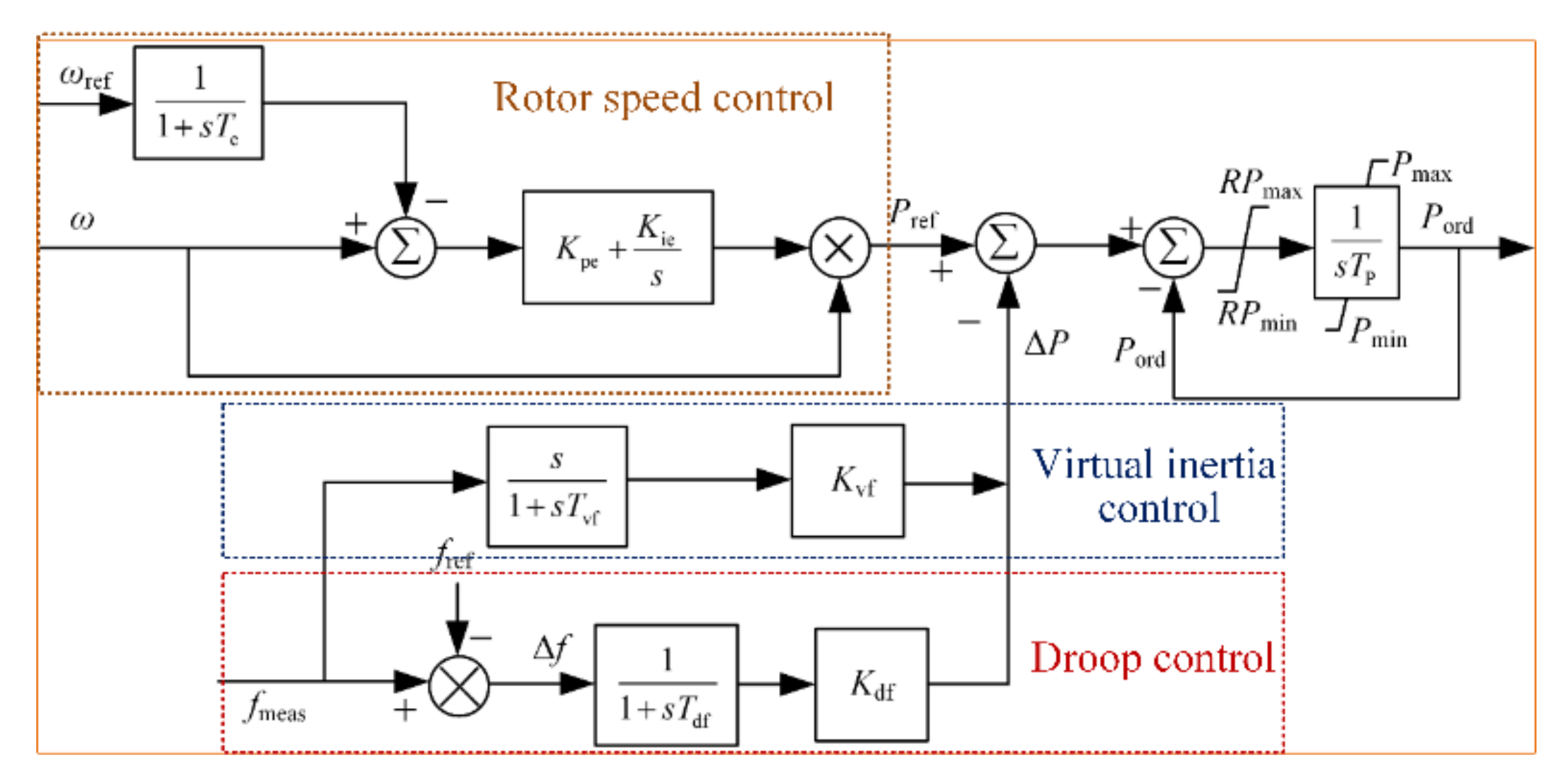
2. DFIG Primary Frequency Regulation Model
2.1. The General Model of DFIG with Frequency Control
2.2. Active Power Control
2.3. Mechanical Power Control Model
3. Equivalent PFR Droop Coefficient of DFIG
3.1. Approximation of Active Power Change
3.1.1. Dynamic Response of Rotor Speed Control
3.1.2. Dynamic Response of Pitch Angle Control
3.1.3. Transform of Integral Terms
3.2. Approximation of Mechanical Power
3.3. Equivalent PFR Droop Coefficient in Fixed-Pitch Angle Mode
3.4. Equivalent PFR Droop Coefficient in Fixed-Rotor Speed Mode
3.5. The Physical Interpretation of the Equivalent Droop Coefficient
4. Influencing Factors of Equivalent Droop Coefficient
4.1. Steady Operating Point
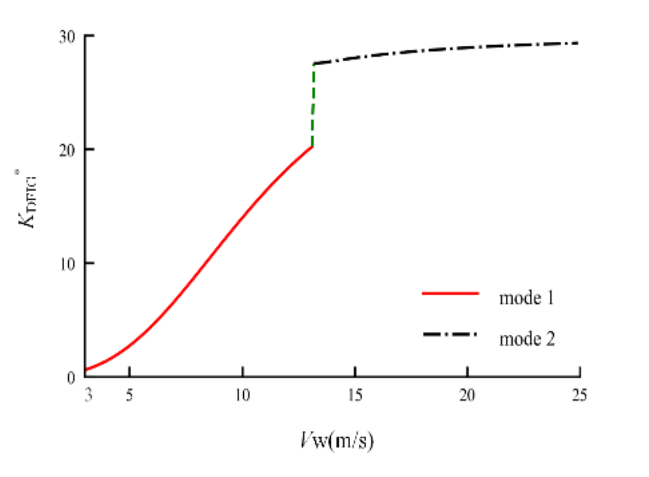
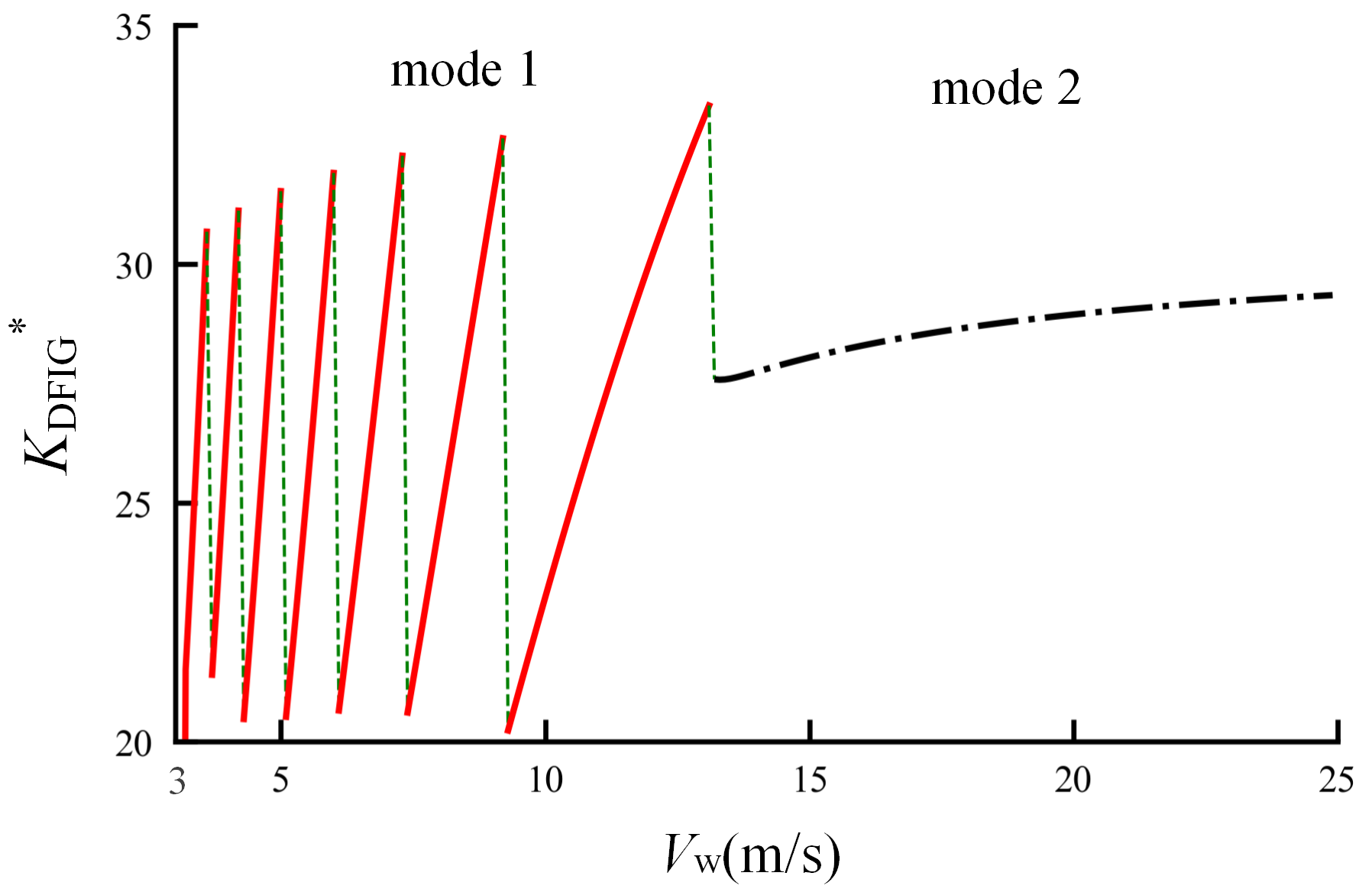
4.1.1. Wind Speed (Vw)
4.1.2. Load Shedding Ratio (d)
4.2. Key Control Parameters
4.3. TE−TP
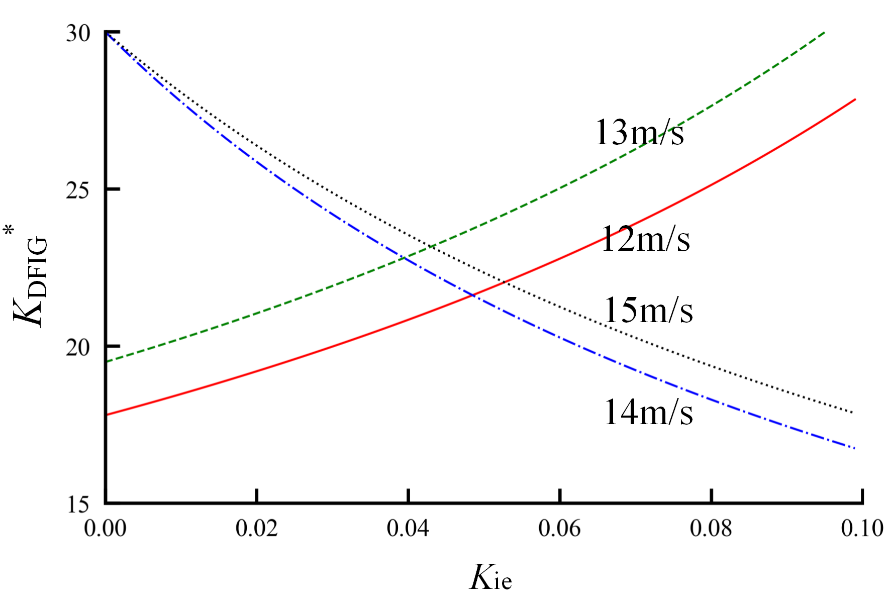
4.4. Kie and Kip
4.5. Optimized Droop Control Coefficient
5. Case Studies
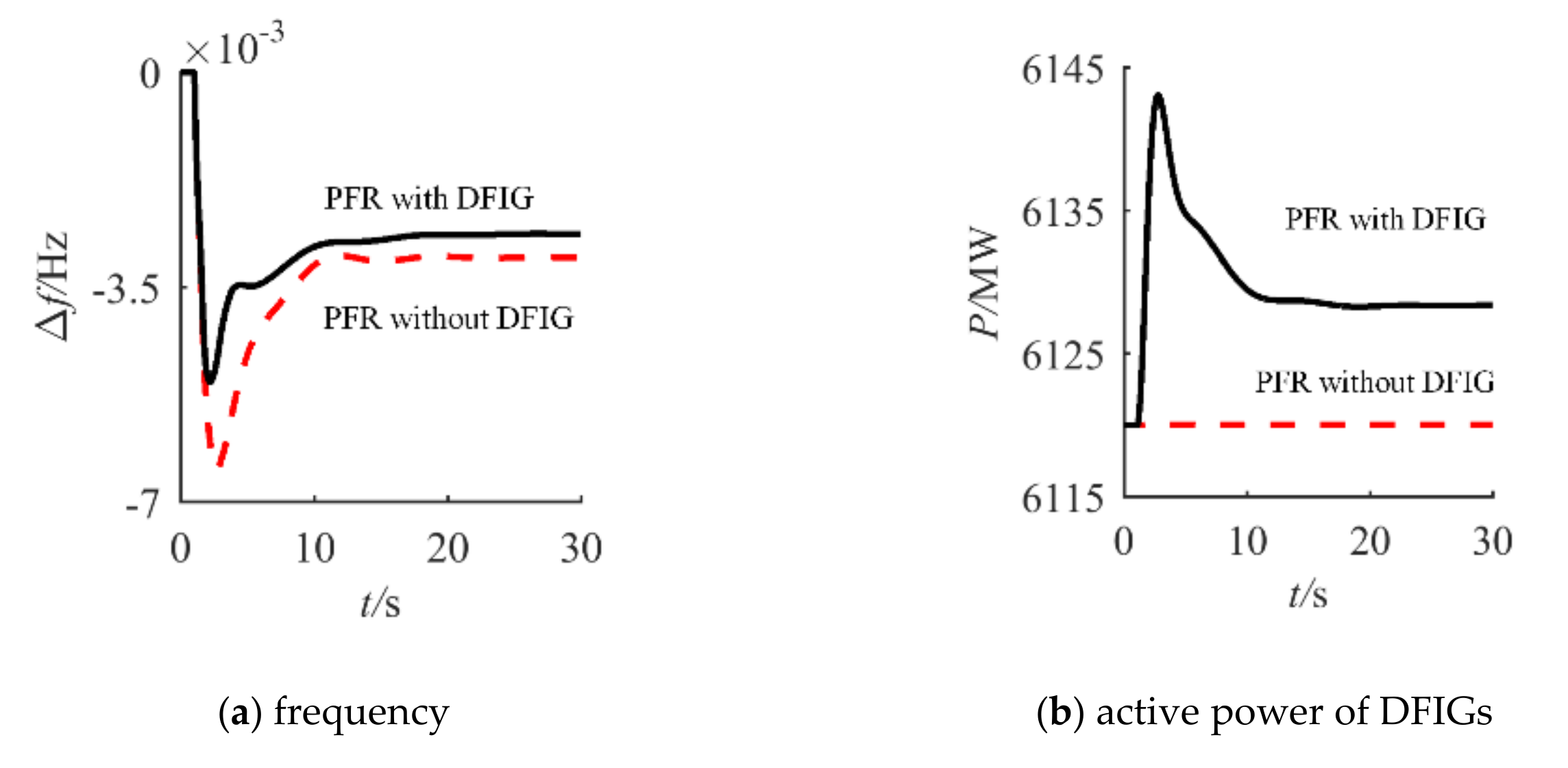
5.1. Cases to Verify the Proposed Method
5.2. PFR Capability with Wind Fluctuation
5.2.1. KDFIG * of Single DFIG under Field Wind Speed
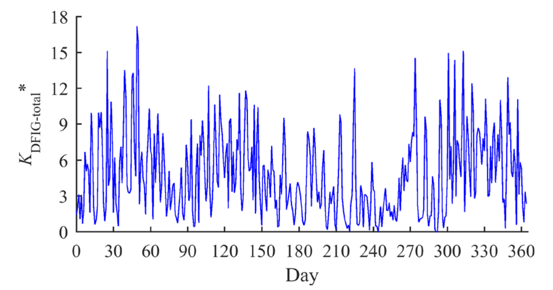
5.2.2. Aggregated KDFIG * of DFIGs in a Province
6. Conclusions
Author Contributions
Funding
Conflicts of Interest
References
- Ding, L.; Yin, S.; Wang, T.X.; Jiang, J.; Cheng, F. Integrated Frequency Control Strategy of DFIGs Based on Virtual Inertia and Over-Speed Control Power System Technology. Power Syst. Technol. 2015, 39, 2385–2391. [Google Scholar]
- Chen, K.; Peng, P.Q.; Li, H.R.; Xu, T.Y.; Li, C.G. DFIG Primary Frequency Regulation Strategy with Optimal Dynamic Droop Control under Variable Wind Speeds. IOP Conf. Ser. Earth Environ. Sci. 2018, 188, 012087. [Google Scholar] [CrossRef]
- Cheng, Y.; Azizipanah-Abarghooee, R.; Azizi, S.; Ding, L.; Terzija, V. Smart Frequency Control in Low Inertia Energy Systems Based on Frequency Response Techniques: A review. Appl. Energy 2020, 279, 115798. [Google Scholar] [CrossRef]
- Li, C.; Wu, Y.; Sun, Y.; Zhang, H.; Liu, Y.; Liu, Y.; Terzija, V. Continuous Under-Frequency Load Shedding for Power System Adaptive Frequency Control. IEEE Trans. Power Syst. 2020, 35, 950–961. [Google Scholar] [CrossRef]
- Mehta, B.; Bhatt, P.; Pandya, V. Small Signal Stability Analysis of Power Systems with DFIG Based Wind Power Penetration. Int. J. Electr. Power Energy Syst. 2014, 58, 64–74. [Google Scholar] [CrossRef]
- Tian, X.; Wang, W.; Chi, Y.; Li, Y.; Liu, C. Adaptation Virtual Inertia Control Strategy of DFIG and Assessment of Equivalent Virtual Inertia Time Constant of Connected Power System. J. Eng. 2017, 2017, 922–928. [Google Scholar] [CrossRef]
- Li, S.; Deng, C.; Shu, Z.; Huang, W.; He, J.; You, Z. Equivalent Inertial Time Constant of Doubly Fed Induction Generator Considering Synthetic Inertial Control. J. Renew. Sustain. Energy 2016, 8, 053304. [Google Scholar] [CrossRef]
- Arani, M.F.M.; Mohamed, Y.A.-R.I. Dynamic Droop Control for Wind Turbines Participating in Primary Frequency Regulation in Microgrids. IEEE Trans. Smart Grid 2018, 9, 5742–5751. [Google Scholar] [CrossRef]
- Vidyanandan, K.V.; Senroy, N. Closure to Discussion on “Primary Frequency Regulation by Deloaded Wind Turbines Using Variable Droop”. IEEE Trans. Power Syst. 2014, 29, 414–415. [Google Scholar] [CrossRef]
- De Almeida, R.G.; Lopes, J.A.P. Participation of Doubly Fed Induction Wind Generators in System Frequency Regulation. IEEE Transactions on Power Syst. 2007, 22, 944–950. [Google Scholar] [CrossRef]
- Zhang, Z.; Sun, Y.; Li, G.; Cheng, L.; Lin, J. Frequency Regulation by Doubly Fed Induction Generator Wind Turbines Based on Coordinated Over-Speed Control and Pitch Control. Autom. Electr. Power Syst. 2011, 35, 20–25. [Google Scholar]
- Mahvash, H.; Taher, S.A.; Rahimi, M.; Shahidehpour, M. Enhancement of DFIG Performance at High Wind Speed Using Fractional Order PI Controller in Pitch Compensation loop. Int. J. Electr. Power Energy Syst. 2019, 104, 259–268. [Google Scholar] [CrossRef]
- Yuan, X.; Li, Y. Control of Variable Pitch and Variable Speed Direct-Drive Wind Turbines in Weak Grid Systems with Active Power Balance. IET Renew. Power Gener. 2014, 8, 119–131. [Google Scholar] [CrossRef]
- Wu, F.; Zhang, X.-P.; Godfrey, K.; Ju, P. Small Signal Stability Analysis and Optimal Control of A Wind Turbine with Doubly Fed Induction Generator. IET Gener. Transm. Distrib. 2007, 1, 751–760. [Google Scholar] [CrossRef]
- Vidyanandan, K.V.; Senroy, N. Primary Frequency Regulation by De-Loaded Wind Turbines Using Variable Droop. IEEE Trans. Power Syst. 2013, 28, 837–846. [Google Scholar] [CrossRef]
- Yang, J.-S.; Chen, Y.-W.; Hsu, Y.-Y. Small-Signal Stability Analysis and Particle Swarm Optimisation Self-Tuning Frequency Control for An Islanding System with DFIG Wind Farm. IET Gener. Transm. Distrib. 2019, 13, 563–574. [Google Scholar] [CrossRef]
- Attya, A.B.; Hartkopf, T. Penetration Impact of Wind Farms Equipped with Frequency Variations Ride Through Algorithm on Power System Frequency Response. Int. J. Electr. Power Energy Syst. 2012, 40, 94–103. [Google Scholar] [CrossRef]
- Ramos, C.J.; Martins, A.P.; Carvalho, A.D.S. Power System Frequency Estimation Using A Least Mean Squares Differentiator. Int. J. Electr. Power Energy Syst. 2017, 87, 166–175. [Google Scholar] [CrossRef]
- Jiang, W.; Lu, J. Frequency Estimation in Wind Farm Integrated Systems Using Artificial Neural Network. Int. J. Electr. Power Energy Syst. 2014, 62, 72–79. [Google Scholar] [CrossRef]
- Polajžer, B.; Dolinar, D.; Ritonja, J. Estimation of Area’s Frequency Response Characteristic During Large Frequency Changes Using Local Correlation. IEEE Trans. Power Syst. 2016, 31, 3160–3168. [Google Scholar] [CrossRef]
- Lam, A.Y.S.; Leung, K.-C.; Li, V.O.K. Capacity Estimation for Vehicle-to-Grid Frequency Regulation Services with Smart Charging Mechanism. IEEE Trans. Smart Grid 2016, 7, 156–166. [Google Scholar] [CrossRef]
- Sun, D.; Sun, L.; Wu, F.; Zu, G. Frequency Inertia Response Control of SCESS-DFIG under Fluctuating Wind Speeds Based on Extended State Observers. Energies 2018, 11, 830. [Google Scholar] [CrossRef]
- Yan, X.; Song, Z.; Xu, Y.; Sun, Y.; Wang, Z.; Sun, X. Study of Inertia and Damping Characteristics of Doubly Fed Induction Generators and Improved Additional Frequency Control Strategy. Energies 2018, 12, 38. [Google Scholar] [CrossRef]
- Abad, G.; López, J.; Rodríguez, M.A.; Marroyo, L.; Iwanski, G. Doubly Fed Induction Machine: Modeling and Control for Wind Energy Generation; John Wiley & Sons, Inc.: Hoboken, NJ, USA, 2011. [Google Scholar]
- Zhang, S.; Mishra, Y.; Yuan, B.; Zhao, J.; Shahidehpour, M. Primary Frequency Controller with Prediction-Based Droop Coefficient for Wind-Storage Systems Under Spot Market Rules. Energies 2018, 11, 2340. [Google Scholar] [CrossRef]
- NASA Power Data Access Viewer. Available online: https://power.larc.nasa.gov/data-access-viewer/ (accessed on 10 September 2020).


| Vm(m/s) | Kdf | KDFIG * |
|---|---|---|
| (3.0,3.6] | 872 | (21.51,33.30] |
| (3.6,4.2] | 560.5 | (21.40,33.32] |
| (4.2,5.0] | 344.3 | (20.47,33.32] |
| (5.0,6.0] | 212.0 | (20.52,33.32] |
| (6.0,7.3] | 131.4 | (20.65,33.31] |
| (7.3,9.2] | 81.3 | (20.61,33.30] |
| (9.2,13.0] | 49.4 | (20.23,33.32] |
| (13.0,25.0) | 30 | (27.58,29.36) |
| Wind Farm(City) | Latitude | Longitude | Installed Capacity |
|---|---|---|---|
| A(Dongying) | 37.55° N | 118.53° E | 150 MW |
| B(Penglai) | 37.80° N | 120.81° E | 150 MW |
| C(Weihai) | 37.49° N | 122.11° E | 200 MW |
| D(Yantai) | 37.52° N | 121.42° E | 200 MW |
| E(Jinan) | 36.66° N | 117.01° E | 300 MW |
| F(Weifang) | 36.71° N | 119.09° E | 200 MW |
| G(Rizhao) | 35.43° N | 119.48° E | 100 MW |
| H(Zibo) | 36.79° N | 118.12° E | 200 MW |
Publisher’s Note: MDPI stays neutral with regard to jurisdictional claims in published maps and institutional affiliations. |
© 2020 by the authors. Licensee MDPI, Basel, Switzerland. This article is an open access article distributed under the terms and conditions of the Creative Commons Attribution (CC BY) license (http://creativecommons.org/licenses/by/4.0/).
Share and Cite
Li, C.; Hang, Z.; Zhang, H.; Guo, Q.; Zhu, Y.; Terzija, V. Evaluation of DFIGs’ Primary Frequency Regulation Capability for Power Systems with High Penetration of Wind Power. Energies 2020, 13, 6178. https://doi.org/10.3390/en13236178
Li C, Hang Z, Zhang H, Guo Q, Zhu Y, Terzija V. Evaluation of DFIGs’ Primary Frequency Regulation Capability for Power Systems with High Penetration of Wind Power. Energies. 2020; 13(23):6178. https://doi.org/10.3390/en13236178
Chicago/Turabian StyleLi, Changgang, Zhi Hang, Hengxu Zhang, Qi Guo, Yihua Zhu, and Vladimir Terzija. 2020. "Evaluation of DFIGs’ Primary Frequency Regulation Capability for Power Systems with High Penetration of Wind Power" Energies 13, no. 23: 6178. https://doi.org/10.3390/en13236178
APA StyleLi, C., Hang, Z., Zhang, H., Guo, Q., Zhu, Y., & Terzija, V. (2020). Evaluation of DFIGs’ Primary Frequency Regulation Capability for Power Systems with High Penetration of Wind Power. Energies, 13(23), 6178. https://doi.org/10.3390/en13236178