Author Contributions
Conceptualization, D.C., D.G. and F.R.; data curation, F.D.P., S.L., E.R. (Elisabetta Ricciardelli) and E.R. (Ermann Ripepi); formal analysis, S.T.N., D.C., D.G., S.G. and E.R. (Elisabetta Ricciardelli); funding acquisition, E.G.; investigation, E.R. (Elisabetta Ricciardelli); Methodology, S.T.N.; project administration, E.G. and F.R.; resources, S.G., E.R. (Ermann Ripepi) and M.V.; software, S.T.N. and F.D.P.; supervision, F.R.; validation, D.C., D.G. and F.R.; visualization, S.T.N.; writing—original draft, S.T.N.; writing—review and editing, D.C., F.D.P., D.G., S.G., E.G., S.L., E.R. (Elisabetta Ricciardelli), E.R. (Ermann Ripepi), M.V. and F.R. All authors have read and agreed to the published version of the manuscript.
Appendix A. Standard Verification Methods for Continuous Variables Forecasts
In this appendix we describe the statistical indexes used for the validation of the WRF outputs forecasts: bias, mean absolute error (MAE), normalized root-mean-square error (nRMSE), correlation coefficient (R), fractional bias (FB), normalized mean square error (nMSE), fraction of predictions within a factor of two of observations (FAC2).
Bias is defined as the sum of the difference between forecasted (
F) and observed (
O) values divided by the total number of samples.
Bias gives an indication of the forecast average error but does not measure the correspondence between forecasts and observations. Bias can assume values between and , perfect score means a bias equal to zero.
Mean Absolute Error (
MAE) is the ratio between the sum of the absolute value of the difference between forecasts (
F) and observations (
O) and the total number of samples.
It is used to address the average magnitude of the forecast errors but does not indicate the direction of them. It can be a value between zero and with perfect score zero.
Normalized Root-Mean-Square Error (
nRMSE) is calculated according to the following formula:
It measures average error weighted according to the square of the error and is normalized by the mean observation value. In particular this index is influenced mainly by large errors encouraging conservative forecasts. It can assume values between 0 and 1 with perfect score 0.
Correlation coefficient is calculated using the following equation:
It is a measure of the phase error. A good correlation coefficient means a scatter plot with values arranged around the diagonal but does not consider the bias and is sensitive to outliers. It can be a value ranging from −1 to 1 with perfect score equivalent to 1. Having a good correlation coefficient is a necessary but not sufficient condition for having a perfect forecast.
Fractional Bias (
FB) is defined as the sum of the difference between observed (
O) and forecasted (F) values divided by the sum of the sum between observed (
O) and forecasted (
F), all divided by 2.
It is a measure of systematic errors and gives an indication on how the forecast underestimate or overestimate the measures. A good forecast means having a FB of 0.
Normalized Mean Square Error (
nMSE) is calculated according to the following formula:
It quantifies random error beyond that systematic error. Perfect score is reached with value equal to zero.
Fraction of predictions within a factor of two of observations (
FAC2) is a robust measure because is not influenced by outliers and is obtained following this criterion:
Appendix B. Standard Verification Methods for Dichotomous Variables Forecasts
In this appendix are described the statistical indexes used for the validation of the multitest based approach fog forecast method: accuracy, bias score, probability of detection (POD), false alarm ration (FAR), probability of false detection (POFD), success ratio (SR), threat score (TS), equitable threat score (ETS), Hanssen and Kuipers discriminant (HKD), Heidke skill score (HSS) and Odds ratio skill score (ORSS).
In order to calculate categorical statistics, first, a contingency table must be defined showing the joint distribution, i.e., the frequency of positive and negative occurrences:
Table A1.
Binary contingency table
Table A1.
Binary contingency table
| | n_total | Observed |
|---|
| Observed Yes | Observed No |
|---|
| Forecasted | Forecast Yes | tp | tn |
| Forecast No | fn | fp |
where:
tp (true positive) or hits are those events that were forecasted and actually occurred;
tn (true negative) or correct negatives are the events that were not forecasted and did not occur;
fp (false positive) or false alarms are those events that were forecasted but not occur;
fn (false negative) or misses are the events occurred but not forecasted; and
n_total is the sum of true positives, true negatives, false positives and false negatives.
Keeping in mind that a perfect system would produce only true positives and true negatives and that in this work a positive event is represented by the correct detection/forecast of fog presence, below there are reported the description of the calculated categorical statistics and the criteria to their interpretation.
Accuracy, or fraction correct, is the ratio between the sum of
hits and
correct negatives and the
n_total. It can assume values ranging from 0 to 1 (best value).
Accuracy gives the fraction of the overall correct forecasts.
Bias score, also called frequency bias, measures the ratio of the frequency of forecasts to the frequency of observations. Can assume values over zero (perfect score is 1). If
BIAS < 1 the system has a tendency of under forecast, the opposite if
BIAS > 1.
Probability of detection (or
true positive rate or
sensitivity) returns the frequency of observed event correctly forecasted. Values ranges from 0 to 1 with 1 perfect score.
POD is sensitive to hits but not consider false alarms.
True negative rate (or
specificity) is the ratio of the true negative by the sum of all negative observed events. It is useful in the determination of ROC (Receiving Operating Characteristic) curve and to calculate the Youden’s index.
False alarm ratio gives an indication on the fraction of positive predicted events actually not occurred. It can assume values between 0 to 1 with 0 perfect score. It is sensitive to false alarms but not to misses.
Probability of false detection (or false alarm rate) is the fraction correct negatives event not forecasted. Values ranges from 0 to 1.
POFD should be 0 in a perfect system.
Success ratio measures the fraction of
hits among all the positive forecasts (sum of
hits and
false alarms).
SR is equal to 1 −
FAR. Value range is between 0 and 1, with 1 best performance indicator.
Threat score (or critical success index-CSI-) is the measurement of the fraction of observed and forecasted events that were correctly predicted. Thus, it differs from the accuracy because it does not consider true negatives. It is sensitive to
hits, A
TS of 0 indicates that the system has no skill while 1 that system is perfect.
Equitable threat score (or Gilbert skill score-GSS-) gives information on how well the positive forecasts correspond to the positive observations adjusted for
hits associated with random chance. It is sensitive to hits and does not distinguish the source of forecast error because it penalizes both misses and false alarms. It assumes values ranging from −1/3 to 1 with 0 and 1 respectively the worst and the best values.
where
Hansen and Kuipers discriminant (also called true skill statistic-TSS-or Peirce’s skill score-PSS-) measures if and how well the system is able to separate positive from negative forecasts. It can be seen also as the difference between
POD and
POFD and interpreted as the sum of accuracy for events and accuracy for no events minus one. It ranges from −1 to 1, 0 indicates no skills and 1 the perfect score.
Heidke skill score (or Cohen’s k) is defined as the fraction of correct forecasts after the elimination of those forecasts which would be correct due purely to random chance. It ranges from −1 to 1, where 0 indicates no skills and 1 the perfect score
with
Odds ratio skill score, i.e., Yule’s, quantifies the improvement of the forecast over the random chance. Values range is from −1 to 1. Zero is the worst while 1 is the best value.
Youden’s index is defined as the difference between true positive rate and false alarm rate.
This index is used to find appropriate cut-off in a categorical forecast. In particular maximum value of Youden’s index allow to select the value that maximize the area under ROC. YI values can range from 0 to 1 with 1 perfect score.
In the theory of decision, ROC curves are graphical schemes for a binary classifier in which are reported the false positive rate on the x-axis and the true positive rate on the y-axis. Best ROC curve has an area under ROC (AROC) of 1, in particular, AROC values around 0.5 means probability of low accurate forecasts and value towards 1 probability of high accurate forecasts.
Appendix C. MBFog Statistical Evaluation with Respect to Other Fog Forecast Methods
In this appendix we report MBFog performances with respect to the following alternative methods available in the open literature:
- (a)
FSI test: Fog Stability Index under a fixed threshold (31), as reported in [
38];
- (b)
RH/Wind test: RH larger than a fixed threshold (90%) and Wind Speed smaller than a fixed threshold (2 ms
−1), as reported in [
34];
- (c)
Visibility test: Visibility obtained from Liquid Water Content (LWC) using Kunkel’s law [
41] less than a fixed threshold (1 km), as reported in [
37,
41].
It is important to remark that all variables used in these comparisons (surface temperature, surface dew point temperature, wind speed at 10 m, temperature at 850 hPa, wind speed at 850 hPa, surface mixing ratio) are obtained from the same IMAA-CNR WRF runs used in MBFog performance evaluation, i.e., daytime hourly outputs of 35 runs selected in the period January–April 2018.
In the following tables all the statistical performances for each of the selected sites are reported. Overall, based on the IMAA-CNR WRF runs outputs, we can conclude that MBFog improves the performance compared to the other considered methods.
Table A2.
Performances of several fog prediction methods for Milano Linate site
Table A2.
Performances of several fog prediction methods for Milano Linate site
| LIML (Milano Linate) |
|---|
| | tp | tn | fp | fn | n_total | Accuracy | BIAS | POD | FAR | POFD | SR | TS | ETS | HKD | HSS | ORSS |
|---|
| (a) | 16 | 100 | 1 | 4 | 141 | 0.82 | 1.85 | 0.8 | 0.57 | 0.17 | 0.43 | 0.39 | 0.30 | 0.63 | 0.46 | 0.9 |
| (b) | 2 | 121 | 0 | 18 | 141 | 0.88 | 0.1 | 0.1 | 0 | 0 | 1 | 0.1 | 0.09 | 0.1 | 0.16 | 1 |
| (c) | 4 | 120 | 1 | 16 | 141 | 0.88 | 0.25 | 0.2 | 0.2 | 0.01 | 0.8 | 0.19 | 0.16 | 0.19 | 0.28 | 0.93 |
| MBFog | 14 | 119 | 2 | 6 | 141 | 0.94 | 0.8 | 0.7 | 0.12 | 0.02 | 0.88 | 0.64 | 0.6 | 0.68 | 0.75 | 0.99 |
Table A3.
Performances of several fog prediction methods for Milano Malpensa site
Table A3.
Performances of several fog prediction methods for Milano Malpensa site
| LIMC (Milano Malpensa) |
|---|
| | tp | tn | fp | fn | n_total | Accuracy | BIAS | POD | FAR | POFD | SR | TS | ETS | HKD | HSS | ORSS |
|---|
| (a) | 7 | 92 | 20 | 1 | 120 | 0.82 | 3.37 | 0.87 | 0.74 | 0.18 | 0.26 | 0.25 | 0.20 | 0.70 | 0.33 | 0.94 |
| (b) | 0 | 111 | 1 | 8 | 120 | 0.92 | 0.12 | 0 | 1 | 0.09 | 0 | 0 | −0.07 | −0.01 | −0.01 | −1 |
| (c) | 3 | 111 | 1 | 5 | 120 | 0.95 | 0.5 | 0.37 | 0.25 | 0.01 | 0.75 | 0.33 | 0.31 | 0.37 | 0.48 | 0.97 |
| MBFog | 7 | 109 | 3 | 1 | 120 | 0.97 | 1.25 | 0.88 | 0.3 | 0.03 | 0.7 | 0.64 | 0.61 | 0.85 | 0.76 | 0.99 |
Table A4.
Performances of several fog prediction methods for Verona site
Table A4.
Performances of several fog prediction methods for Verona site
| LIPX (Verona) |
|---|
| | tp | tn | fp | fn | n_total | Accuracy | BIAS | POD | FAR | POFD | SR | TS | ETS | HKD | HSS | ORSS |
|---|
| (a) | 10 | 99 | 7 | 5 | 121 | 0.9 | 1.13 | 0.67 | 0.41 | 0.07 | 0.59 | 0.45 | 0.4 | 0.6 | 0.57 | 0.93 |
| (b) | 1 | 106 | 0 | 14 | 121 | 0.88 | 0.07 | 0.07 | 0 | 0 | 1 | 0.07 | 0.06 | 0.07 | 0.11 | 1 |
| (c) | 2 | 105 | 1 | 13 | 121 | 0.88 | 0.2 | 0.13 | 0.33 | 0.01 | 0.67 | 0.12 | 0.10 | 0.12 | 0.19 | 0.88 |
| MBFog | 12 | 104 | 2 | 3 | 121 | 0.96 | 0.93 | 0.8 | 0.14 | 0.02 | 0.86 | 0.71 | 0.67 | 0.78 | 0.8 | 0.99 |
Table A5.
Performances of several fog prediction methods for Venezia site
Table A5.
Performances of several fog prediction methods for Venezia site
| LIPZ (Venezia) |
|---|
| | tp | tn | fp | fn | n_total | Accuracy | BIAS | POD | FAR | POFD | SR | TS | ETS | HKD | HSS | ORSS |
|---|
| (a) | 12 | 110 | 1 | 0 | 136 | 0.9 | 2.17 | 1 | 0.54 | 0.11 | 0.46 | 0.46 | 0.41 | 0.89 | 0.58 | 1 |
| (b) | 3 | 124 | 0 | 9 | 136 | 0.93 | 0.25 | 0.25 | 0 | 0 | 1 | 0.25 | 0.23 | 0.25 | 0.38 | 1 |
| (c) | 7 | 121 | 3 | 5 | 136 | 0.94 | 0.83 | 0.58 | 0.3 | 0.02 | 0.7 | 0.47 | 0.43 | 0.56 | 0.6 | 0.97 |
| MBFog | 11 | 122 | 2 | 0 | 136 | 0.99 | 1.17 | 1 | 0.14 | 0.02 | 0.86 | 0.86 | 0.84 | 0.98 | 0.91 | 1 |
Table A6.
Performances of several fog prediction methods for Bologna site
Table A6.
Performances of several fog prediction methods for Bologna site
| LIPE (Bologna) |
|---|
| | tp | tn | fp | fn | n_total | Accuracy | BIAS | POD | FAR | POFD | SR | TS | ETS | HKD | HSS | ORSS |
|---|
| (a) | 3 | 108 | 21 | 1 | 133 | 0.83 | 6 | 0.75 | 0.87 | 0.16 | 0.12 | 0.12 | 0.09 | 0.59 | 0.17 | 0.88 |
| (b) | 1 | 129 | 0 | 3 | 133 | 0.98 | 0.25 | 0.25 | 0 | 0 | 1 | 0.25 | 0.24 | 0.25 | 0.39 | 1 |
| (c) | 1 | 119 | 10 | 3 | 133 | 0.9 | 2.75 | 0.25 | 0.91 | 0.08 | 0.09 | 0.07 | 0.05 | 0.17 | 0.09 | 0.6 |
| MBFog | 3 | 127 | 2 | 1 | 133 | 0.98 | 1.25 | 0.75 | 0.4 | 0.02 | 0.6 | 0.5 | 0.49 | 0.73 | 0.66 | 0.99 |
Table A7.
Performances of several fog prediction methods for Ferrara site
Table A7.
Performances of several fog prediction methods for Ferrara site
| LIPF (Ferrara) |
|---|
| | tp | tn | fp | fn | n_total | Accuracy | BIAS | POD | FAR | POFD | SR | TS | ETS | HKD | HSS | ORSS |
|---|
| (a) | 29 | 84 | 22 | 5 | 140 | 0.81 | 1.5 | 0.85 | 0.43 | 0.21 | 0.57 | 0.52 | 0.38 | 0.65 | 0.55 | 0.91 |
| (b) | 3 | 105 | 1 | 31 | 140 | 0.77 | 0.12 | 0.09 | 0.25 | 0.01 | 0.75 | 0.09 | 0.06 | 0.08 | 0.11 | 0.82 |
| (c) | 12 | 104 | 2 | 22 | 140 | 0.83 | 0.41 | 0.35 | 0.14 | 0.02 | 0.86 | 0.33 | 0.26 | 0.33 | 0.42 | 0.93 |
| MBFog | 22 | 104 | 2 | 12 | 140 | 0.9 | 0.71 | 0.65 | 0.08 | 0.02 | 0.92 | 0.61 | 0.54 | 0.63 | 0.7 | 0.98 |
Table A8.
Performances of several fog prediction methods for Frontone site
Table A8.
Performances of several fog prediction methods for Frontone site
| LIVF (Frontone) |
|---|
| | tp | tn | fp | fn | n_total | Accuracy | BIAS | POD | FAR | POFD | SR | TS | ETS | HKD | HSS | ORSS |
|---|
| (a) | 2 | 17 | 0 | 10 | 29 | 0.66 | 0.17 | 0.17 | 0 | 0 | 1 | 0.17 | 0.1 | 0.17 | 0.19 | 1 |
| (b) | 0 | 16 | 0 | 12 | 29 | 0.55 | 0.08 | 0 | 1 | 0.06 | 0 | 0 | −0.03 | −0.06 | −0.07 | −1 |
| (c) | 7 | 15 | 2 | 5 | 29 | 0.76 | 0.75 | 0.58 | 0.22 | 0.12 | 0.78 | 0.5 | 0.32 | 0.47 | 0.48 | 0.83 |
| MBFog | 12 | 16 | 1 | 0 | 29 | 0.97 | 1.08 | 1 | 0.08 | 0.06 | 0.92 | 0.92 | 0.87 | 0.94 | 0.93 | 1 |
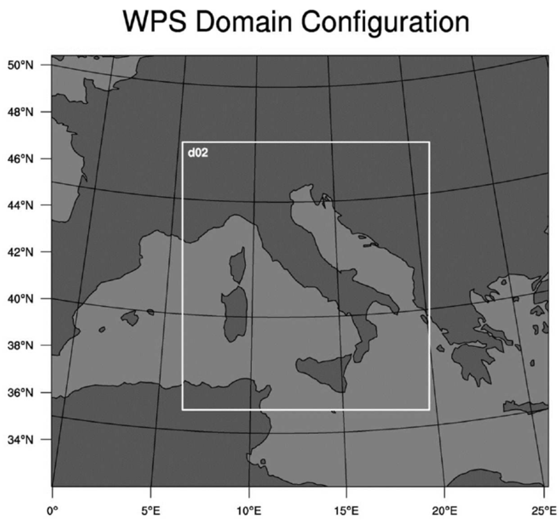
Figure 1.
Spatial domains of the Weather Research and Forecasting (WRF) model running at the Institute of Methodologies for Environmental Analysis of the National Research Council of Italy (IMAA-CNR).
Figure 1.
Spatial domains of the Weather Research and Forecasting (WRF) model running at the Institute of Methodologies for Environmental Analysis of the National Research Council of Italy (IMAA-CNR).
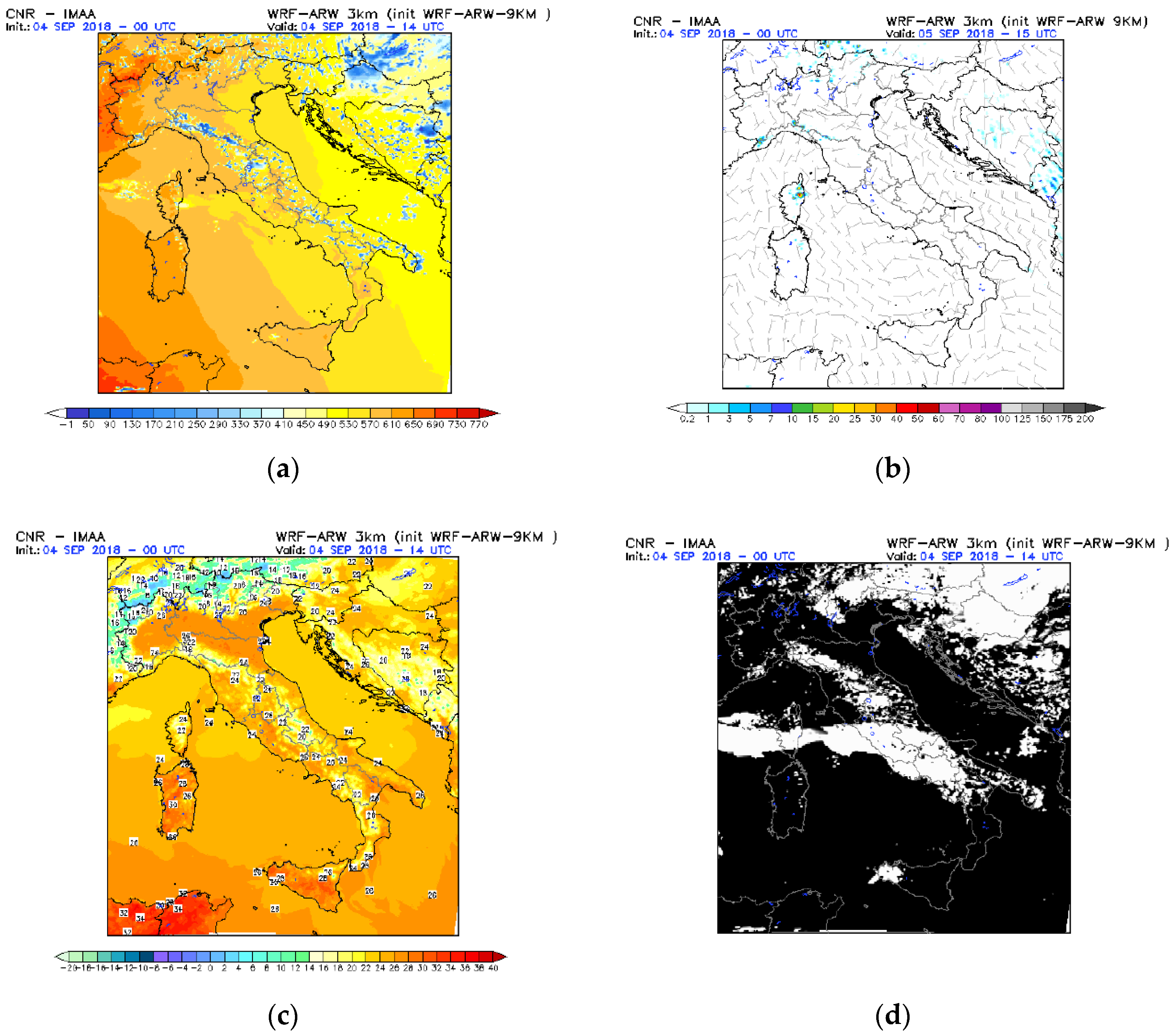
Figure 2.
Example of IMAA-CNR WRF products. Run of 04/09/18 at 00:00 UTC, forecast valid at 14:00 UTC on 04 September 18. Variables forecasted: (a) global horizontal irradiance (W/m2), (b) 3 h cumulated total precipitation (mm/3 h) plus wind speed (knots) and direction, (c) surface temperature (°C), (d) cloud cover.
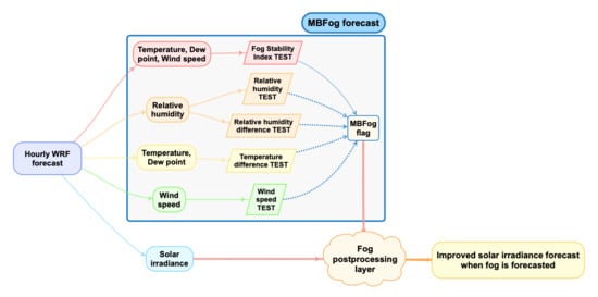
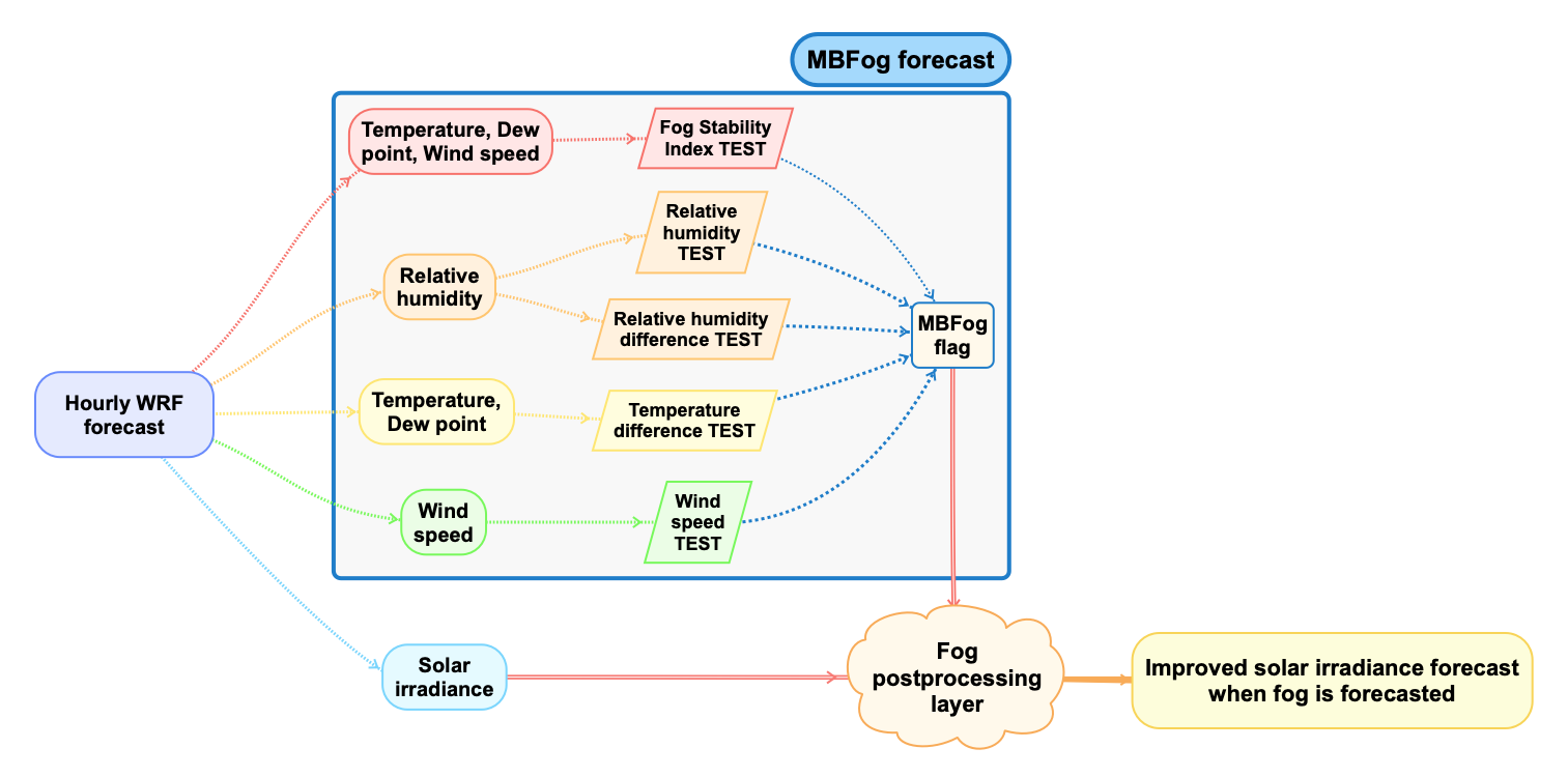
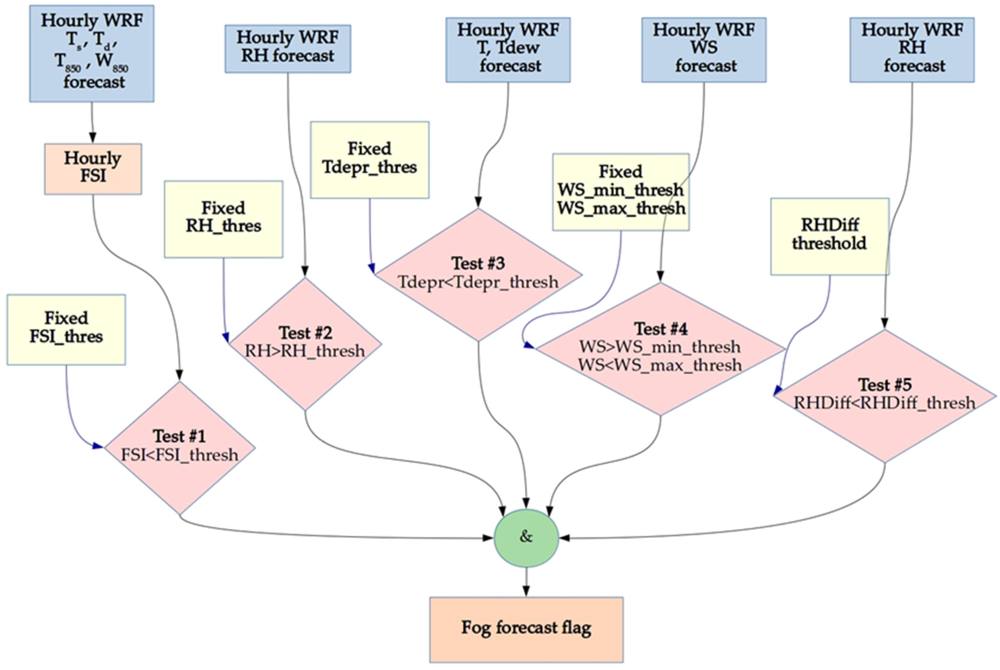
Figure 3.
Block diagram of the multitest-based method for forecasting fog (MBFog) using WRF output. Thresholds are fixed after site-specific climatological study (test #2, #3, #4), statistical study (test #1) or literature review (test #5).
Figure 3.
Block diagram of the multitest-based method for forecasting fog (MBFog) using WRF output. Thresholds are fixed after site-specific climatological study (test #2, #3, #4), statistical study (test #1) or literature review (test #5).
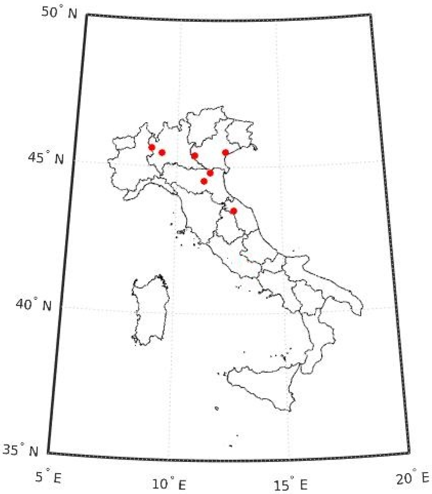
Figure 4.
Map position of the seven sites selected for fog forecast.
Figure 4.
Map position of the seven sites selected for fog forecast.
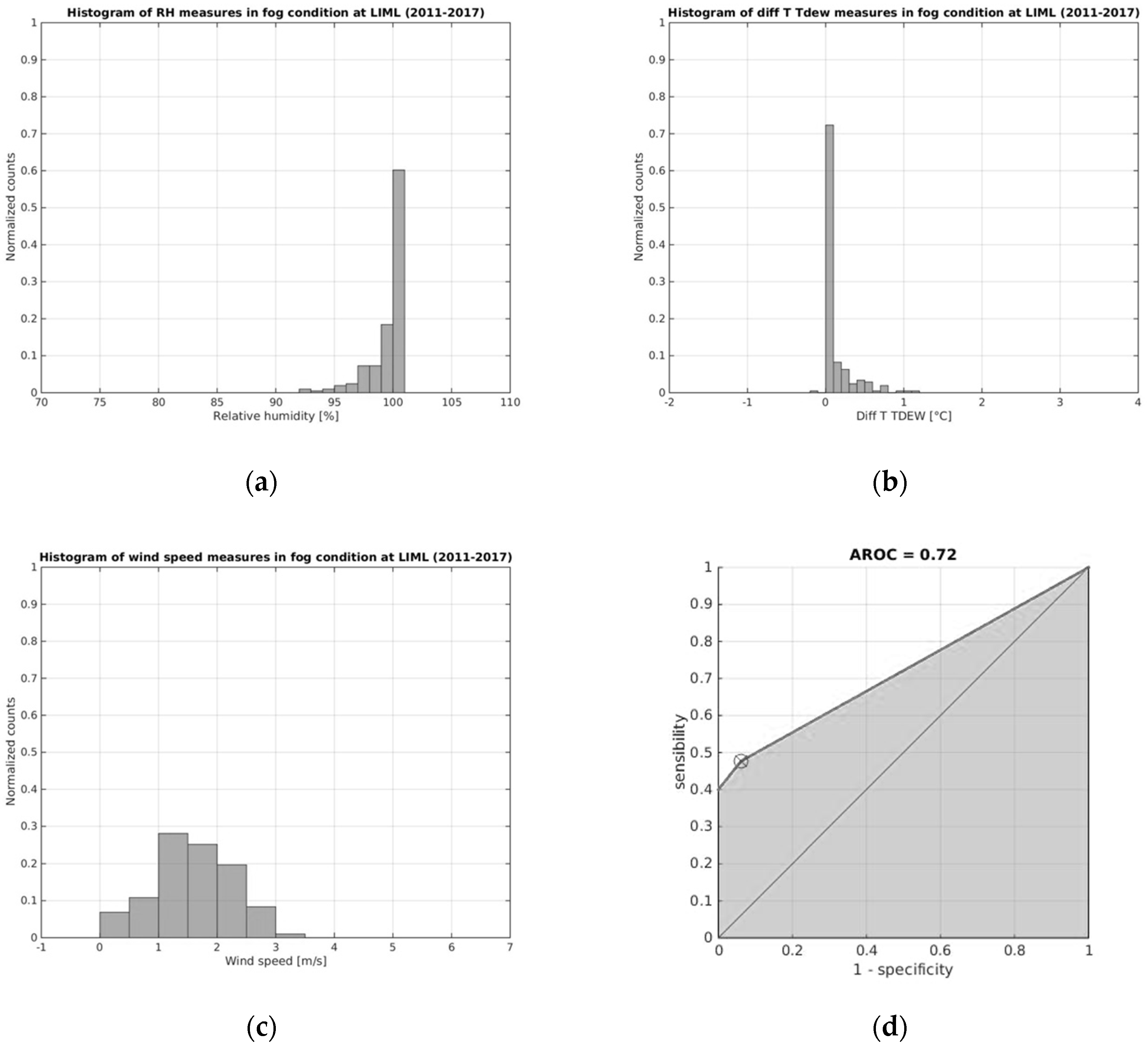
Figure 5.
Histograms of the measurements of (a) relative humidity, (b) surface temperature/dew point difference, (c) wind speed in fog condition at Milano Linate in the period January 2011–December 2017 and (d) receiving operating characteristic (ROC) curve with FSI_thresh = 28.
Figure 5.
Histograms of the measurements of (a) relative humidity, (b) surface temperature/dew point difference, (c) wind speed in fog condition at Milano Linate in the period January 2011–December 2017 and (d) receiving operating characteristic (ROC) curve with FSI_thresh = 28.
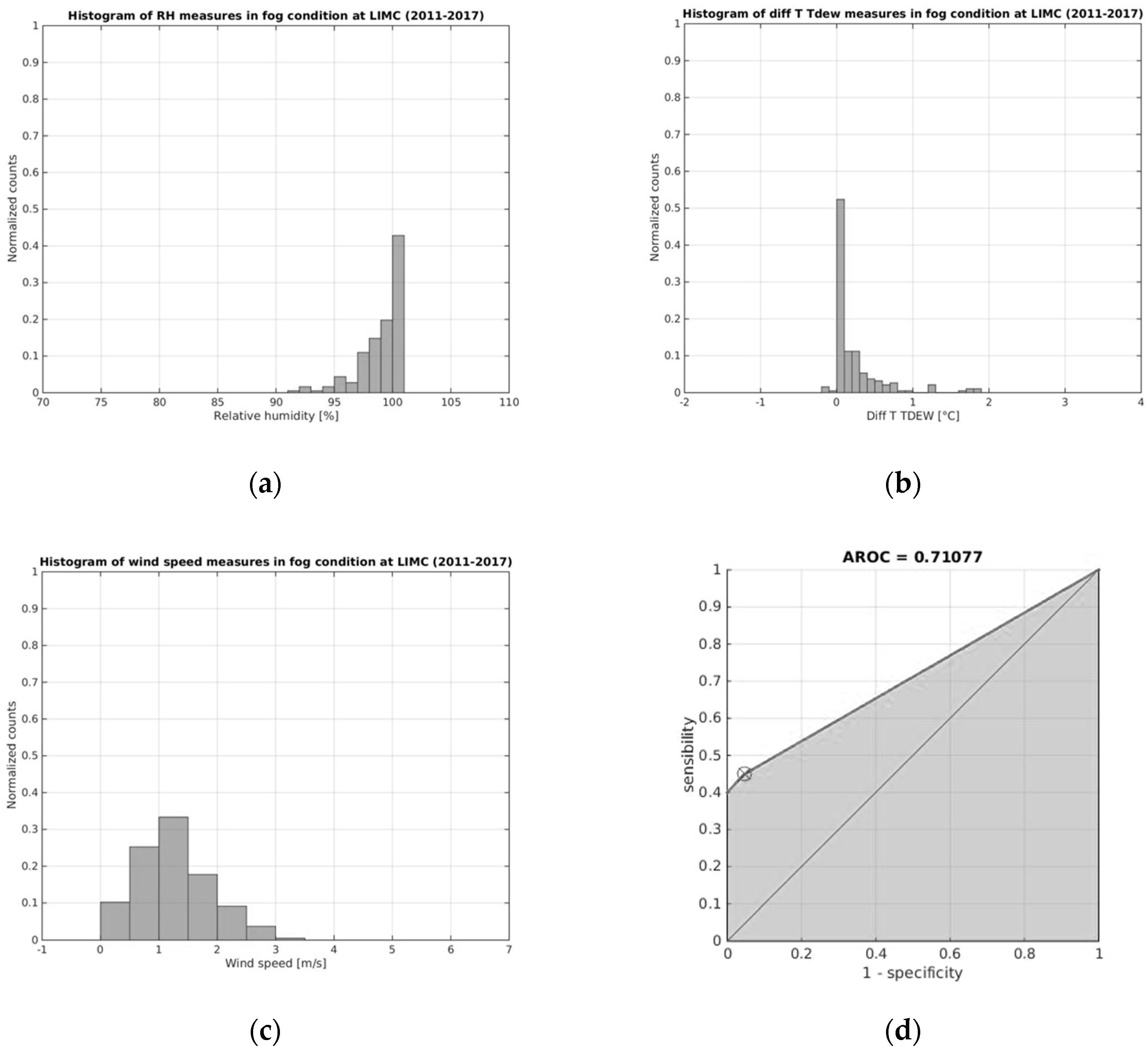
Figure 6.
Histograms of the measurements of (a) relative humidity, (b) surface temperature/dew point difference, (c) wind speed in fog condition at Milano Malpensa in the period January 2011–December 2017 and (d) ROC curve with FSI_thresh = 26.
Figure 6.
Histograms of the measurements of (a) relative humidity, (b) surface temperature/dew point difference, (c) wind speed in fog condition at Milano Malpensa in the period January 2011–December 2017 and (d) ROC curve with FSI_thresh = 26.
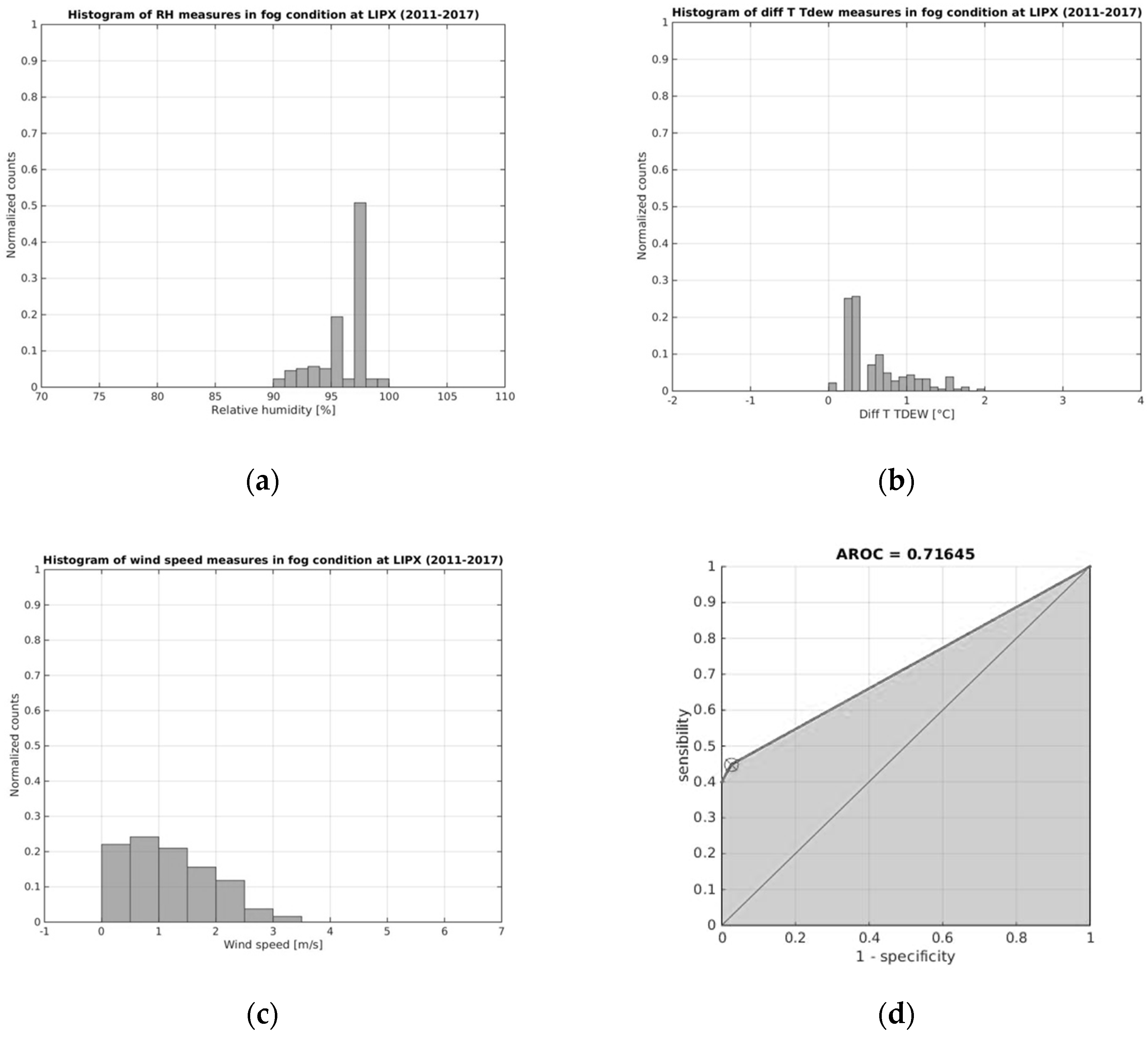
Figure 7.
Histograms of the measurements of (a) relative humidity, (b) surface temperature/dew point difference, (c) wind speed in fog condition at Verona in the period January 2011–December 2017 and (d) ROC curve with FSI_thresh = 26.
Figure 7.
Histograms of the measurements of (a) relative humidity, (b) surface temperature/dew point difference, (c) wind speed in fog condition at Verona in the period January 2011–December 2017 and (d) ROC curve with FSI_thresh = 26.
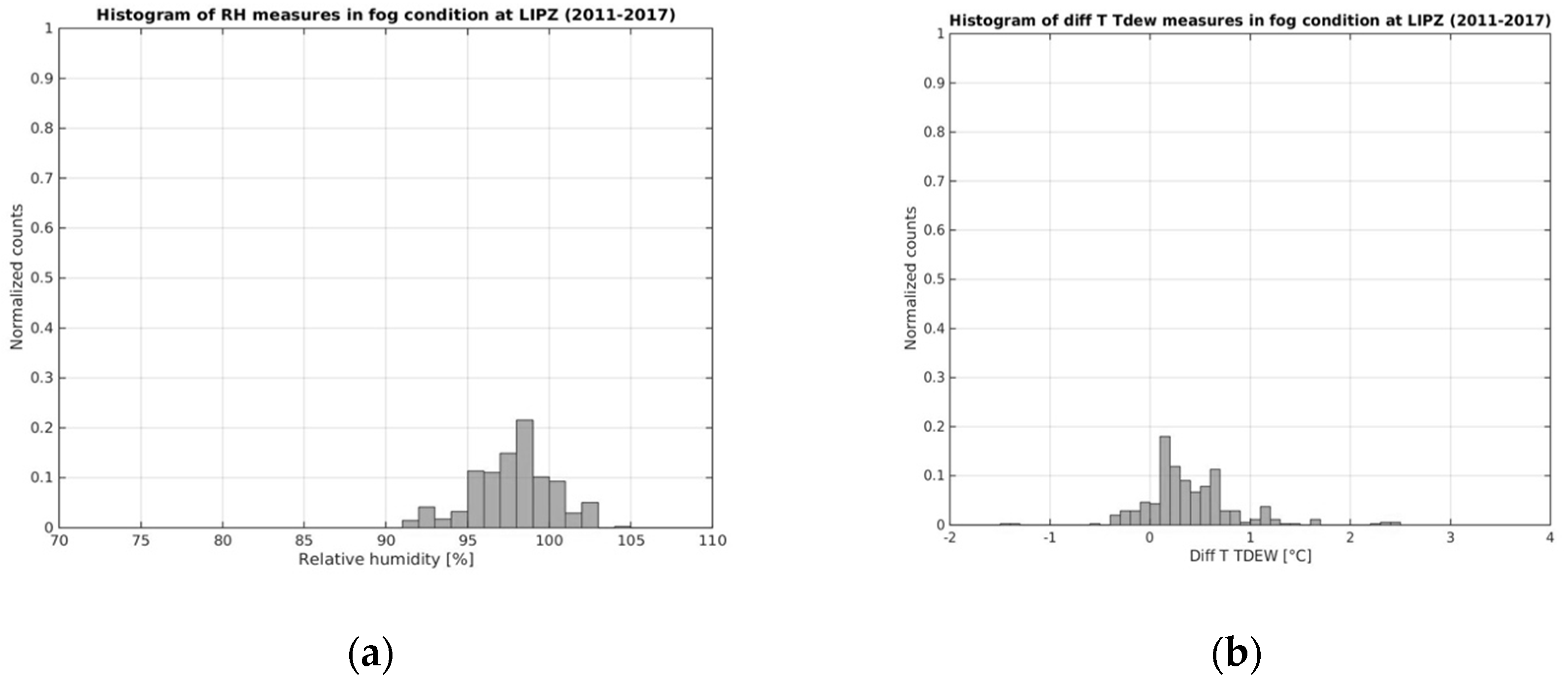
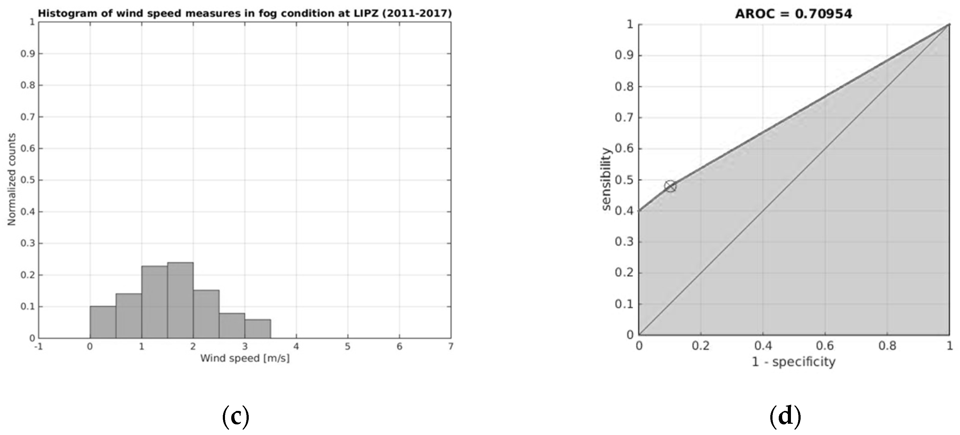
Figure 8.
Histograms of the measurements of (a) relative humidity, (b) surface temperature/dew point difference, (c) wind speed in fog condition at Venezia in the period January 2011–December 2017 and (d) ROC curve with FSI_thresh = 27.
Figure 8.
Histograms of the measurements of (a) relative humidity, (b) surface temperature/dew point difference, (c) wind speed in fog condition at Venezia in the period January 2011–December 2017 and (d) ROC curve with FSI_thresh = 27.
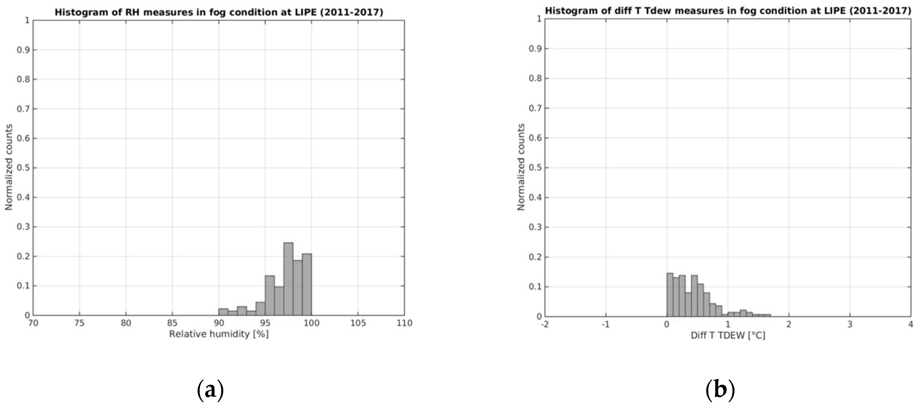
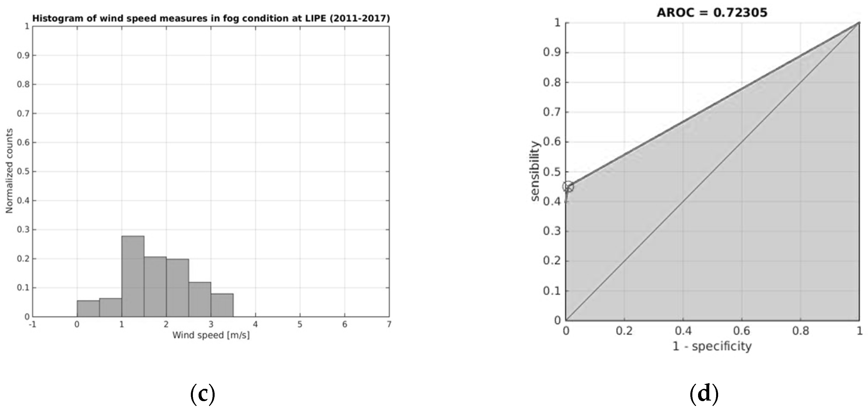
Figure 9.
Histograms of the measurements of (a) relative humidity, (b) surface temperature/dew point difference, (c) wind speed in fog condition at Bologna in the period January 2011–December 2017 and (d) ROC curve obtained with FSI_thresh = 24.
Figure 9.
Histograms of the measurements of (a) relative humidity, (b) surface temperature/dew point difference, (c) wind speed in fog condition at Bologna in the period January 2011–December 2017 and (d) ROC curve obtained with FSI_thresh = 24.
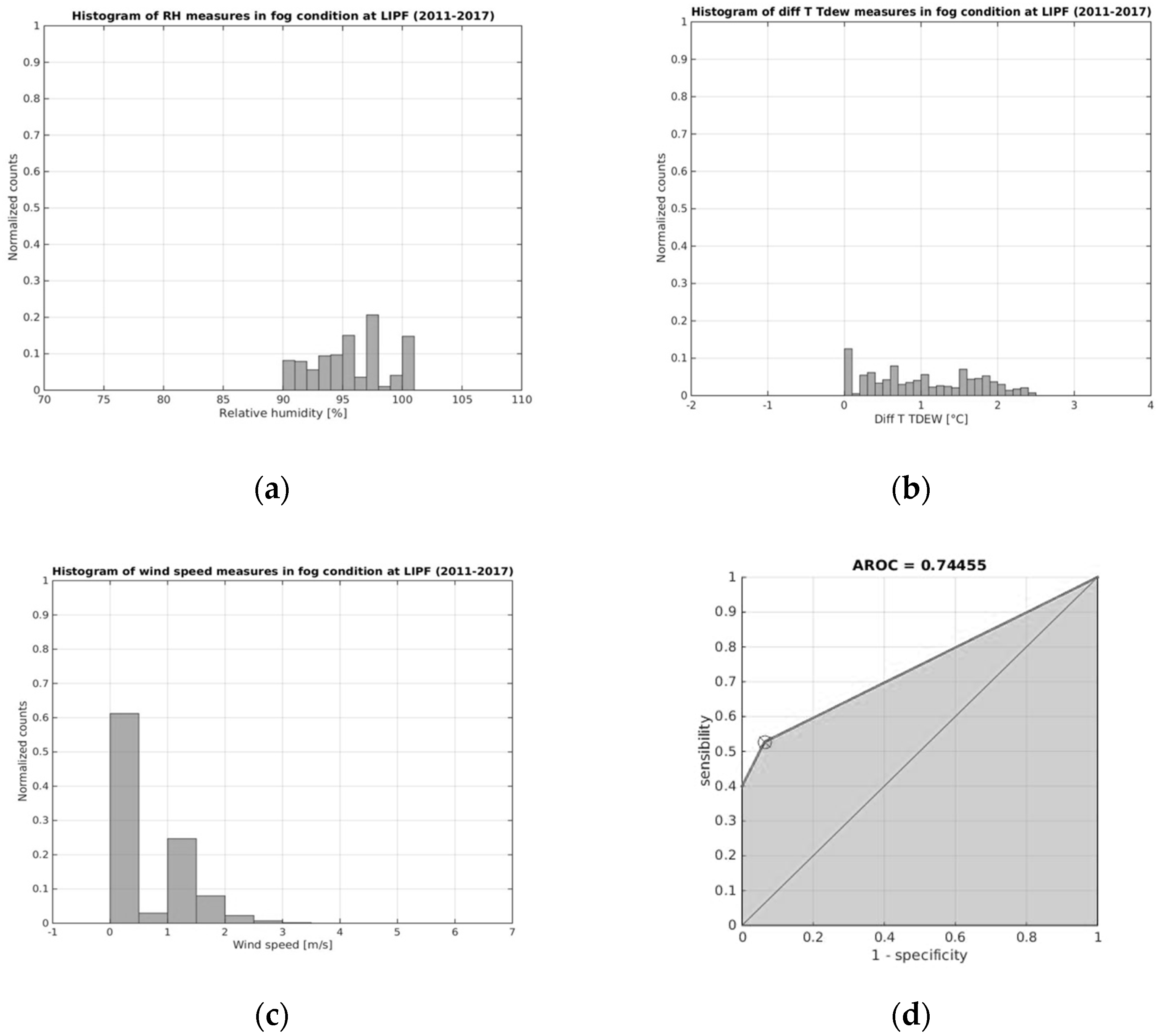
Figure 10.
Histograms of the measurements of (a) relative humidity, (b) surface temperature/dew point difference, (c) wind speed in fog condition at Ferrara in the period January 2011–December 2017 and (d) ROC curve obtained with FSI_thresh = 25.
Figure 10.
Histograms of the measurements of (a) relative humidity, (b) surface temperature/dew point difference, (c) wind speed in fog condition at Ferrara in the period January 2011–December 2017 and (d) ROC curve obtained with FSI_thresh = 25.
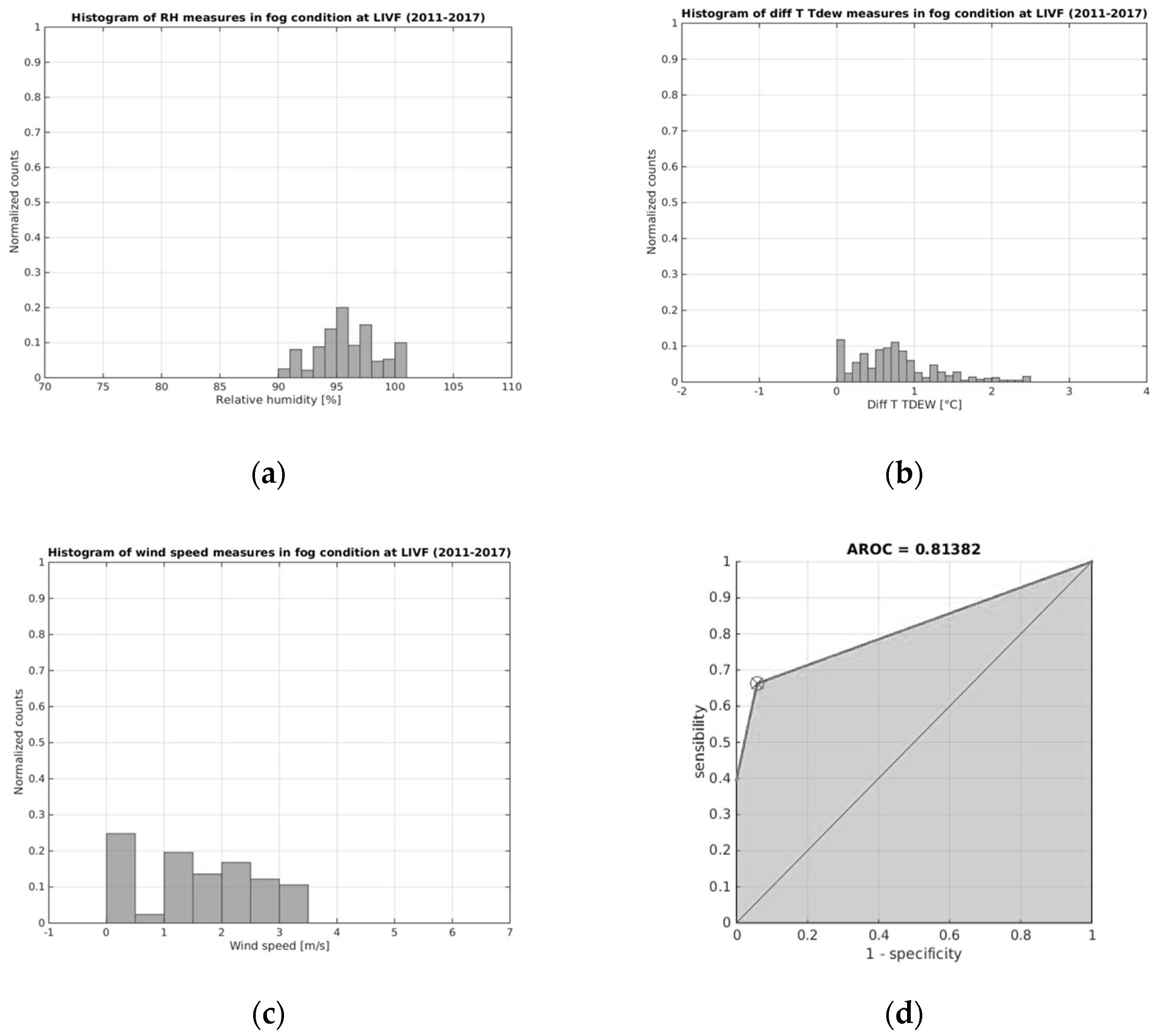
Figure 11.
Histograms of the measurements of (a) relative humidity, (b) surface temperature/dew point difference, (c) wind speed in fog condition at Frontone in the period January 2011–December 2017 and (d) ROC curve obtained with FSI_thresh = 32.
Figure 11.
Histograms of the measurements of (a) relative humidity, (b) surface temperature/dew point difference, (c) wind speed in fog condition at Frontone in the period January 2011–December 2017 and (d) ROC curve obtained with FSI_thresh = 32.
Table 1.
List of sites used for WRF outputs performance evaluation and relative number of samples used for validation.
Table 1.
List of sites used for WRF outputs performance evaluation and relative number of samples used for validation.
| Longitude (°) | Latitude (°) | IATA Code | City | Samples |
|---|
| 8.72396 E | 45.63 N | LIMC | Milano Malpensa | 321 |
| 9.2626 E | 45.46143 N | LIML | Milano Linate | 318 |
| 11.29694 E | 44.53083 N | LIPE | Bologna | 321 |
| 11.6125 E | 44.81556 N | LIPF | Ferrara | 220 |
| 10.87228 E | 45.38749 N | LIPX | Verona Villafranca | 310 |
| 12.35194 E | 45.50528 N | LIPZ | Venezia | 313 |
| 12.72778 E | 43.51694 N | LIVF | Frontone | 86 |
Table 2.
Statistical scores of WRF surface temperature outputs related to the seven selected sites measurements. (A negative BIAS means a WRF underestimation and vice versa).
Table 2.
Statistical scores of WRF surface temperature outputs related to the seven selected sites measurements. (A negative BIAS means a WRF underestimation and vice versa).
| | Surface Temperature |
|---|
| | N | BIAS (°C) | MAE (°C) | nRMSE | R | FB | FAC2 |
|---|
| Milano Linate | 12 | 0.21 | 0.88 | 0.08 | 0.99 | −0.004 | 1 |
| Milano Malpensa | 15 | 0.29 | 0.74 | 0.08 | 0.99 | −0.01 | 0.87 |
| Verona | 17 | −0.15 | 1.39 | 0.11 | 0.98 | 0.03 | 0.94 |
| Venezia | 17 | 0.58 | 0.81 | 0.12 | 0.98 | −0.02 | 1 |
| Bologna | 6 | −0.30 | 0.7 | 0.1 | 0.98 | 0.01 | 1 |
| Ferrara | 6 | −1.05 | 1.71 | 0.21 | 0.97 | 0.03 | 1 |
| Frontone | 4 | 1.17 | 1.99 | 0.29 | 0.89 | 0.07 | 1 |
Table 3.
Statistical scores of WRF surface dew point outputs related to the seven selected sites measurements. (A negative BIAS means a WRF underestimation and vice versa).
Table 3.
Statistical scores of WRF surface dew point outputs related to the seven selected sites measurements. (A negative BIAS means a WRF underestimation and vice versa).
| | Surface Dew Point |
|---|
| N | BIAS (°C) | MAE (°C) | nRMSE | R | FB | FAC2 |
|---|
| Milano Linate | 15 | 0.98 | 2.03 | 0.63 | 0.91 | −0.06 | 0.66 |
| Milano Malpensa | 12 | 1.49 | 1.68 | 1.6 | 0.93 | −0.19 | 0.4 |
| Verona | 13 | 0.07 | 1.43 | 0.54 | 0.97 | −0.01 | 0.93 |
| Venezia | 17 | 1.12 | 1.46 | 0.92 | 0.88 | −0.09 | 0.78 |
| Bologna | 6 | −0.07 | 0.79 | 0.35 | 0.96 | 0.007 | 0.83 |
| Ferrara | 6 | 0.63 | 1.62 | 0.17 | 0.88 | 0.17 | 0.75 |
| Frontone | 4 | 0.80 | 1.06 | 1.4 | 0.91 | −0.07 | 0.72 |
Table 4.
Statistical scores of WRF surface relative humidity outputs of the seven selected sites (a negative BIAS means a WRF underestimation and vice versa).
Table 4.
Statistical scores of WRF surface relative humidity outputs of the seven selected sites (a negative BIAS means a WRF underestimation and vice versa).
| | Surface Relative Humidity |
|---|
| N | BIAS (%) | MAE (%) | nRMSE | R | FB | FAC2 |
|---|
| Milano Linate | 12 | 3.87 | 9.16 | 0.21 | 0.86 | −0.01 | 1 |
| Milano Malpensa | 15 | 3.28 | 4.63 | 0.09 | 0.98 | −0.01 | 1 |
| Verona | 13 | 3.11 | 7.87 | 0.46 | 0.91 | 0.001 | 1 |
| Venezia | 17 | 3.22 | 8.03 | 0.16 | 0.79 | −0.01 | 1 |
| Bologna | 6 | 0.36 | 1.14 | 0.02 | 0.99 | −0.001 | 1 |
| Ferrara | 6 | 6.5 | 6.5 | 0.13 | 0.92 | 0.02 | 1 |
| Frontone | 4 | 3.61 | 8.55 | 0.10 | 0.89 | 0.01 | 1 |
Table 5.
Statistical scores of WRF wind speed at 10 m outputs of the seven selected sites. (a negative BIAS means a WRF underestimation and vice versa).
Table 5.
Statistical scores of WRF wind speed at 10 m outputs of the seven selected sites. (a negative BIAS means a WRF underestimation and vice versa).
| | Wind Speed at 10 m |
|---|
| N | BIAS (m/s) | MAE (m/s) | nRMSE | R | FB | FAC2 |
|---|
| Milano Linate | 12 | −0.13 | 0.93 | 1.15 | 0.26 | 0.17 | 0.67 |
| Milano Malpensa | 15 | −1.12 | 1.67 | 0.82 | 0.45 | 0.10 | 0.67 |
| Verona | 13 | −0.42 | 1.14 | 0.62 | 0.63 | 0.05 | 0.69 |
| Venezia | 17 | 0.39 | 1.16 | 0.72 | 0.70 | 0.18 | 0.41 |
| Bologna | 6 | −0.44 | 0.93 | 0.48 | 0.29 | 0.05 | 0.66 |
| Ferrara | 6 | 1.73 | 1.81 | 1.19 | 0.38 | −0.16 | 0.67 |
| Frontone | 4 | −0.19 | 1.25 | 1.04 | 0.64 | 0.04 | 0.72 |
Table 6.
Mean, standard deviation and thresholds selected for relative humidity, surface temperature/dew point depression and wind speed measured in fog condition and FSI threshold calculated using Youden’s index for Milano Linate.
Table 6.
Mean, standard deviation and thresholds selected for relative humidity, surface temperature/dew point depression and wind speed measured in fog condition and FSI threshold calculated using Youden’s index for Milano Linate.
| | Mean | Standard Deviation | Threshold |
|---|
| RH | 99.30% | 3.40% | Min: 98% |
| Diff_T_TDEW | 0.10 °C | 0.21 °C | Max: 1.2 °C |
| WS10 | 1.43 m/s | 0.75 m/s | Min: 0 m/s
Max: 1.3 m/s |
| FSI | - | - | 28 |
Table 7.
Mean, standard deviation and thresholds selected for relative humidity, surface temperature/dew point depression and wind speed measured in fog condition and fog stability index (FSI) threshold calculated using Youden’s index for Milano Malpensa.
Table 7.
Mean, standard deviation and thresholds selected for relative humidity, surface temperature/dew point depression and wind speed measured in fog condition and fog stability index (FSI) threshold calculated using Youden’s index for Milano Malpensa.
| | Mean | Standard Deviation | Threshold |
|---|
| RH | 98.6% | 4.5% | Min: 99% |
| Diff_T_TDEW | 0.22 °C | 0.37 °C | Max: 1.6 °C |
| WS10 | 1.07 m/s | 0.68 m/s | Min: 0 m/s
Max: 1.3 m/s |
| FSI | - | - | 26 |
Table 8.
Mean, standard deviation and thresholds selected for relative humidity, surface temperature/dew point depression and wind speed measured in fog condition and FSI threshold calculated using Youden’s index for Verona.
Table 8.
Mean, standard deviation and thresholds selected for relative humidity, surface temperature/dew point depression and wind speed measured in fog condition and FSI threshold calculated using Youden’s index for Verona.
| | Mean | Standard Deviation | Threshold |
|---|
| RH | 95.54% | 3.58% | Min: 96% |
| Diff_T_TDEW | 0.66 °C | 0.57 °C | Max: 1.9 °C |
| WS10 | 1.01 m/s | 0.84 m/s | Min: 0 m/s
Max: 1.3 m/s |
| FSI | - | - | 26 |
Table 9.
Mean, standard deviation and thresholds selected for relative humidity, surface temperature/dew point depression and wind speed measured in fog condition and FSI threshold calculated using Youden’s index for Venezia.
Table 9.
Mean, standard deviation and thresholds selected for relative humidity, surface temperature/dew point depression and wind speed measured in fog condition and FSI threshold calculated using Youden’s index for Venezia.
| | Mean | Standard Deviation | Threshold |
|---|
| RH | 96.15% | 9.24% | Min: 91% |
| Diff_T_TDEW | 0.65 °C | 0.87 °C | Max: 2.3 °C |
| WS10 | 1.44 m/s | 0.9 m/s | Min: 1.1 m/s
Max: 2.9 m/s |
| FSI | - | - | 27 |
Table 10.
Mean, standard deviation and thresholds selected for relative humidity, surface temperature/dew point depression and wind speed measured in fog condition and FSI threshold calculated using Youden’s index for Bologna.
Table 10.
Mean, standard deviation and thresholds selected for relative humidity, surface temperature/dew point depression and wind speed measured in fog condition and FSI threshold calculated using Youden’s index for Bologna.
| | Mean | Standard Deviation | Threshold |
|---|
| RH | 96.86% | 2.75% | Min: 95% |
| Diff_T_TDEW | 0.45 °C | 0.4 °C | Max: 0.5 °C |
| WS10 | 1.82 m/s | 1.05 m/s | Min: 0.3 m/s
Max: 2.4 m/s |
| FSI | - | - | 24 |
Table 11.
Mean, standard deviation and thresholds selected for relative humidity, surface temperature/dew point depression and wind speed measured in fog condition and FSI threshold calculated using Youden’s index for Ferrara.
Table 11.
Mean, standard deviation and thresholds selected for relative humidity, surface temperature/dew point depression and wind speed measured in fog condition and FSI threshold calculated using Youden’s index for Ferrara.
| | Mean | Standard Deviation | Threshold |
|---|
| RH | 92.98% | 4.75% | Min: 91% |
| Diff_T_TDEW | 1.07 °C | 0.75 °C | Max: 1 °C |
| WS10 | 0.49 m/s | 0.71 m/s | Min: 0.7 m/s
Max: 2.1 m/s |
| FSI | - | - | 25 |
Table 12.
Mean, standard deviation and thresholds selected for relative humidity, surface temperature/dew point depression and wind speed measured in fog condition and FSI threshold calculated using Youden’s index for Frontone.
Table 12.
Mean, standard deviation and thresholds selected for relative humidity, surface temperature/dew point depression and wind speed measured in fog condition and FSI threshold calculated using Youden’s index for Frontone.
| | Mean | Standard Deviation | Threshold |
|---|
| RH | 94.9% | 3.71% | Min: 95% |
| Diff_T_TDEW | 0.78 °C | 0.6 °C | Max: 2.4 °C |
| WS10 | 1.78 m/s | 1.39 m/s | Min: 0 m/s
Max: 2.5 m/s |
| FSI | - | - | 32 |
Table 13.
Overall statistic performances of multitest fog forecast method for the selected sites.
Table 13.
Overall statistic performances of multitest fog forecast method for the selected sites.
| | Milano Linate | Milano Malpensa | Verona | Venezia | Bologna | Ferrara | Frontone |
|---|
| tp | 14 | 7 | 12 | 11 | 3 | 22 | 12 |
| tn | 119 | 109 | 104 | 122 | 127 | 104 | 16 |
| fp | 2 | 3 | 2 | 2 | 2 | 2 | 1 |
| fn | 6 | 1 | 3 | 0 | 1 | 12 | 0 |
| n_total | 141 | 120 | 121 | 136 | 133 | 140 | 29 |
| Accuracy | 0.94 | 0.97 | 0.96 | 0.99 | 0.98 | 0.90 | 0.97 |
| BIAS | 0.80 | 1.25 | 0.93 | 1.17 | 1.25 | 0.71 | 1.08 |
| POD | 0.70 | 0.88 | 0.80 | 1 | 0.75 | 0.65 | 1 |
| FAR | 0.12 | 0.30 | 0.14 | 0.14 | 0.40 | 0.08 | 0.08 |
| POFD | 0.02 | 0.03 | 0.02 | 0.02 | 0.02 | 0.02 | 0.06 |
| SR | 0.88 | 0.70 | 0.86 | 0.86 | 0.60 | 0.92 | 0.92 |
| TS | 0.64 | 0.64 | 0.71 | 0.86 | 0.50 | 0.61 | 0.92 |
| ETS | 0.59 | 0.61 | 0.67 | 0.84 | 0.49 | 0.54 | 0.87 |
| HKD | 0.68 | 0.85 | 0.78 | 0.98 | 0.73 | 0.63 | 0.94 |
| HSS | 0.75 | 0.76 | 0.80 | 0.91 | 0.66 | 0.70 | 0.93 |
| ORSS | 0.99 | 0.99 | 0.99 | 1 | 0.99 | 0.98 | 1 |
Table 14.
Comparison of GHI WRF output performances with or without the application of fog postprocessing layer (ppl).
Table 14.
Comparison of GHI WRF output performances with or without the application of fog postprocessing layer (ppl).
| | Milano Linate | Milano Malpensa | Bologna | Ferrara |
|---|
| No fog ppl | With fog ppl | No fog ppl | With fog ppl | No fog ppl | With fog ppl | No fog ppl | With fog ppl |
|---|
| n_total | 23 | 23 | 15 | 15 | 14 | 14 | 41 | 41 |
| BIAS (W·m−2) | 89.44 | 23.49 | 80.98 | 49.42 | 88.62 | 26.02 | 82.73 | 17.60 |
| MAE (W·m−2) | 89.96 | 31.11 | 80.98 | 49.42 | 88.62 | 27.12 | 102.12 | 44.03 |
| RMSE (W·m−2) | 122.68 | 39.97 | 118.58 | 76.4 | 125.47 | 36.36 | 139.28 | 59.89 |
| R | 0.83 | 0.96 | 0.80 | 0.86 | 0.79 | 0.98 | 0.63 | 0.80 |
| FB | −0.15 | −0.05 | −0.25 | −0.20 | −0.14 | −0.05 | −0.14 | −0.04 |
| nMSE | 0.45 | 0.06 | 1.22 | 0.63 | 0.46 | 0.05 | 0.70 | 0.19 |
| FAC2 | 0.52 | 0.78 | 0.13 | 0.27 | 0.36 | 0.93 | 0.56 | 0.73 |

 ,
, 


