Abstract
Effectively avoiding methane accidents is vital to the security of manufacturing minerals. Coal mine methane accidents are often caused by a methane concentration overrun, and accurately predicting methane emission quantity in a coal mine is key to solving this problem. To maintain the concentration of methane in a secure range, grey theory and neural network model are increasingly used to critically forecasting methane emission quantity in coal mines. A limitation of the grey neural network model is that researchers have merely combined the conventional neural network and grey theory. To enhance the accuracy of prediction, a modified grey GM (1,1) and radial basis function (RBF) neural network model is proposed, which combines the amended grey GM (1,1) model and RBF neural network model. In this article, the proposed model is put into a simulation experiment, which is built based on Matlab software (MathWorks.Inc, Natick, Masezius, U.S). Ultimately, the conclusion of the simulation experiment verified that the modified grey GM (1,1) and RBF neural network model not only boosts the precision of prediction, but also restricts relative error in a minimum range. This shows that the modified grey GM (1,1) and RBF neural network model can make more effective and precise predict the predicts, compared to the grey GM (1,1) model and RBF neural network model.
1. Introduction
Throughout the years, coal mines have played a crucial role in energy resources around the world. Ranking first in coal production, China is the largest consumer of coal all over the world—consuming roughly half of the world’s coal consumption. Coal exploitation has made an important contribution to developing China’s economy by providing employment opportunities and generating purchasing power. Coal still plays a dominant role in the total primary energy, even though coal production is declining in China [1,2]. Nevertheless, the production system in underground coal mines is a peculiarly complex disaster system, which causes coal mine accidents to frequently occur [3].
Safe production in underground coal mines is threatened by a wide variety of coal mine disasters. In China, high rates of coal mine accidents cause huge losses to the Chinese economy, and are responsible for thousands of fatalities among coal miners every year [4]. Among various types of coal mine accidents, methane accidents are normally perceived as the most hazardous [5]. After , methane is the second-biggest source of global greenhouse methane emission; and a main source of methane emission is coal mines [6,7,8].
Studies have shown that methane emission, relevant to coal-mine ventilation, has an adverse impact on the environment. In addition, methane is a precious resource, but it is a serious waste when it is released into the atmosphere [9,10]. Methane emission from the ventilation system is the primary source of coal mine methane emission. In China, approximately 85–90% of coal mine methane is from underground coal mines [11].
Moreover, methane is a highly explosive gas [12]. Therefore, taking advantage of drained methane from coal mines becomes critical when trying to lessen methane emission into the atmosphere [13].
In China, coal and methane outbursts are the most common cause that can rapidly let out large amounts of coal methane, and induce a methane explosion. Intense and sudden releases of coal and methane from coal mines have given rise to equipment damage and casualties [14,15,16].
The data used in Figure 1 comes from the state administration of coal mine safety, which publishes the number of accidents of Chinese situation of coal and methane outburst from 2006 to 2015 [17].
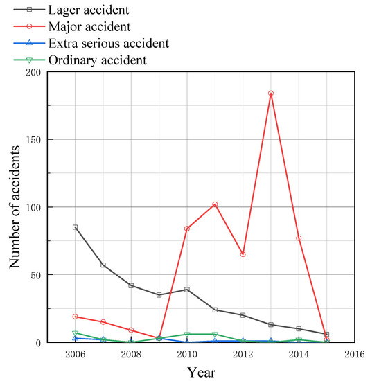
Figure 1.
Chinese coal and methane outbursts from 2006 to 2015.
Between 1950–2015, extremely serious methane explosion disasters have frequently occurred in China. In this time, the number of extremely serious methane explosion disasters reached 126 [18]. Hence, it is necessary to carry out an investigation that can accurately predict methane outbursts, and provide guides for coal mine support.
The energy contained in methane is in direct proportion to its risk degree. For this reason, it is becoming more popular in the energy sector [19]. Indeed, abundant methane released during mining may create security problems, but coal mine enterprises can also obtain obvious economic benefits if they use coal mine methane rationally [20]. On account of the low concentration of methane, some researchers focused on technologies of treating and recovering methane effectively [21]. Meanwhile, in contrast to traditional fossil fuel energy, methane is a cleaner energy resource.
China is the largest coal producer all over the world, in excess of 95% of the national coal production from the underground coal mine. Furthermore, comparing surface mines, underground coal mines have higher methane emissions. An enormous amount of methane is released during the mining process, especially from state-owned coal mines, which have high-methane content. An estimated amount of 19 billion cubic meters of methane discharged from China’s coal mine every year, leading the world, but a few pockets of methane were utilized [11,22,23,24,25].
Methane is categorized as an important greenhouse gas. To protect the atmosphere, it is important that methane is extracted effectively [26]. However, reality dictates that during the process of mining, a considerable amount of coal mine methane just be discharged into the atmosphere through the ventilation system, meaning some of the unused extracted methane is also released [9]. This leads to global warming and energy waste. Previous research has shown that methane concentration that exceeds the limit is commonly triggered by high methane emission. In addition, excessive methane concentration will lead to many serious consequences, such as fire and explosion [27]. Coal mine accidents that are caused by methane are extremely dangerous and increase of depth of the exploited seam—resulting in an increase of methane content. Predicting methane emission is crucial to imposing restrictions on transfinite methane concentration [28].
In spite of methane being present in nearly all coal mines in China, it is unrealistic to use other energy in lieu of coal in recent years. Mining excavations not only affect economic development, but are also inseparable from the people’s livelihood. According to statistics, coal account for 70% of the gross energy supply in China [29]. To guarantee a regular national economy, declining the methane emission and improving the utility ratio of extracted methane are appropriate.
Methane emission is admittedly considered as a significant parameter of methane accidents, and has dramatically impacted the mining process and the mine ventilation design [30]. Hence, to achieve safety production, it is necessary to analyze data in terms of methane emission, and forecast its change tendency in advance.
For the sake of processing complex and enormous data connected with methane emission, various forecasting approaches are proposed. Computational fluid dynamic (CFD) analysis is used to simulate methane emission in underground coal mines [31].
As early as the 1996s, researchers have suggested methods to forecast methane emissions that is associated with disturbed and undisturbed longwall faces [32]. With the rapid development of computer technology in recent years, numerical simulations were widely used to predict methane emissions.
In order to predict methane emission quantity precisely, a time series analysis on the strength of the Gaussian process regression model has been used for methane emission prediction [33]. Moreover, study [34] considered the steeply inclined and extremely thick coal seams, a used new method (that employed numerical simulation), which was applied to forecasting methane emission quantity. The issue related to methane emissions in a multifarious geospatial context was analyzed in Reference [35].
Some researchers have used several kinds of mathematical models to predict and analyze methane emissions simultaneously. Wei et al. focused on methane emission prediction based on a grey prediction model, new information model, and a metabolism model, and compared the results of these three prediction models [36]. Jing et al. simultaneously used model GM (1,1) of grey, and one element linear regression forecasting methane emission, and concluded that the former has a greater precision by contrast [30].
In this study, one improved radial basis function (RBF) neural network model of methane emissions from underground coal mine of China’s Shanxi Province is applied to forecast. Our analysis includes six main affecting factors of methane emissions (coal seam thickness, coal seam spacing, coal seam depth, coal seam methane content, daily production, and daily progress). By processing these factors, a tool used in prediction (associated with methane emission model) was built by the artificial neural network. Predictions of methane emission are presented in this paper, and the prediction accuracy is also discussed. Moreover, this paper compares predicted values with actual values.
2. Methods
2.1. RBF Neural Network
An RBF neural network is a model based on Cover which can use primary function approximating arbitrary function.
where , andrepresent input vector, output vector and NO. i node, respectively. is the centre and express NO. i primary function. represent the weight between the hidden layer and output layer, and i, as well as j, express NO. i of hidden layer, and NO. j node of output layer. is Euclidean norm. N is the number of centers and hidden layer node. is primary function of hidden layer.
To solve output vector , parameters in the Equation (1) should be confirmed which are , and .
The center of RBF neural network can be determined by means of K-means algorithm. It is considering that the elect center can simplify network. Thus, the data that are selected as RBF neural network center should immensely reduce number of elements in the hidden layer.
Confirming radius should guarantee the space of training sample, which can be contained by the set of acceptance region of RBF unit. The general method for determining and is done by employing a K-means algorithm, as shown in Equation (2).
Then, we used a linear least square method adjust weight between the hidden layer and output layer, through Equations (3) and (4).
It is a common practice to consider Gaussian function as , as shown in Equation (5).
where represent input vector and is NO. i perceptive variate which defines width. In this equation express center and subscript i represent NO. i primary function. N is the number of nodes in hidden layer.
Eventually, the output vector can be ciphered out though Equation (6)
2.2. Grey Prediction Model
The grey prediction model is to process the seemingly irregular data column into a regular data column, using a certain method. Therefore, the grey prediction model generates a new sequence and sequence model.
Modified grey forecasting model GM (1,1) is a valid model of bating the randomness of sample data and enhancing accuracy in forecasting methane emission quantity. The first step is to acquire data of factors that can influence methane emission quantity.
Using a computing logarithmic [10] is an eminent way to make data smoother, and improves the accuracy of prediction. This algorithm is shown below. There are x groups training samples and y groups predicted samples, compute logarithmic of these x + y groups of samples. Take methane emission quantity for example:
Then, obtaining x + y groups samples, respectively, are . Among these samples, correspond six influence factors about methane emission quantity, including thickness of coal seam, interval of coal seam, depth of coal seam, concentration of coal seam, daily output, daily progress. Moreover, methane emission quantity homologous sample is .
Secondly, a grey predicted model will be built. The most familiar method to establish grey system model is accumulation.
Adding up x groups of training samples receive a list of data: . Then, we used this data as an input vector for the modified RBF neural network model.
By using grey forecasting model GM (1,1) dispose series. Firstly, we built a differential equation.
Then, to solve the parameters in this equation, we utilize the least square method:
where B and are built by and severally.
Finally, to obtain, the objective vector of modified RBF neural network model, we establish the GM (1,1) model:
The calculated objective vector and input vector were then input into the modified network model for training.
2.3. Modified RBF Neural Network
The improved RBF Neural Network Structure is shown in Figure 2.
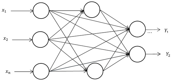
Figure 2.
Improved radial basis function (RBF) neural network structure.
- (1)
- Determine the width of the Gaussian function, δ, set a variable A (1) used to store the sum of heterogeneous outputs, and set a variable B (1) used to count the heterogeneous samples, where 1 is the number of classes.
- (2)
- With , as the first sequence, a network is established, and there is only one hidden neuron node in the network. Let , , , is the center of the hidden layer node, and the weight of the hidden layer node to the output layer is: .
- (3)
- For the second sequence, , calculate the distance between and : . If , then is the nearest neighbor clustering of , and let , , ; If , let , ,. is the hidden node center. A neuron node is added to the hidden layer of step (2), and the weight from the node to the output layer is .
- (4)
- The sequence: , the number of nodes in the hidden layer of the network is , in which the center of the node is in order, and the distance between and is calculated, in turn, . Let .If , then is the nearest-neighbor clustering of , let , , ; and then, , let , remain unchanged, ;If , let , , and let: when , , remain unchanged, add a node to the existing hidden layer of the network, the weight of this node to the output layer: . Repeat the above steps until the sample classification is completed.
- (5)
- Initialize and . is the input layer to output layer weight, is the output layer offset, and there is a random number in the range [0, 1].
- (6)
- Add incentives , as the input of node at time .
- (7)
- Calculation output.Let the output of the node of the hidden layer be:The network output is:
- (8)
- Adjustment weight.The objective function is:Adjust the weights , , and to obtain the increment factor by the gradient descent method, where:The iteration formula to get weights and biases is:Among them:, hidden layer output , represents column of , represents column of , , , , , in turn, indicate the number of input layer, hidden layer and output layer nodes, represents the learning rate, ; α is the momentum factor and ; is the number of iterations.
- (9)
- Go to the next sample and repeat steps (6) to (9), until the error reaches the specified accuracy.
2.4. Modeling and Prediction of Improved Grey RBF Neural Network Model
The modeling and prediction steps, and the structure of the improved grey RBF neural network model are shown in Figure 3 and Figure 4. The modeling prediction steps are as follows:
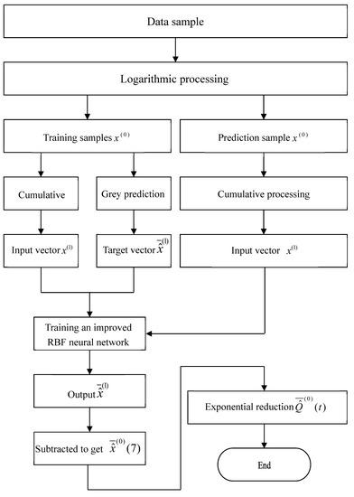
Figure 3.
Improved grey RBF neural network modeling and prediction process.
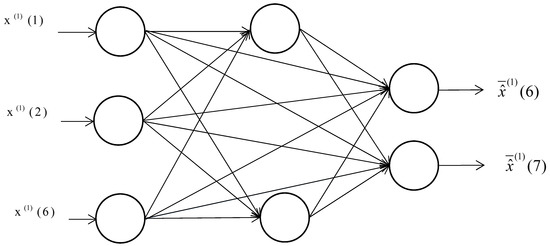
Figure 4.
Improved grey RBF neural network structure diagram.
- (1)
- Group x is the training sample and group y is the prediction sample. Obtaining by evaluating the logarithm of the sample x + y, where in the y group is not processed, , respectively, correspond to the six main factors affecting the methane emission amount, and corresponds to the methane emission amount;
- (2)
- The x group of training samples is accumulated once to obtain , this data is listed as the input vector of the improved RBF neural network model;
- (3)
- The data column is predicted by the GM (1,1) model to obtain , , and , as the target vector;
- (4)
- Input the input vector and target vector in (2) and (3) into the improved RBF neural network training;
- (5)
- The y group of prediction samples is accumulated once to obtain ;
- (6)
- Input obtained in step (5) into the improved RBF neural network trained in step (4), and obtain predicted values , ;
- (7)
- Find the difference: ;
- (8)
- Index reduction: , is the final predicted value of methane emission.
3. Results and Discussion
In order to test the prediction effect of the model, this paper uses 300 sets of methane data from a coal mine in Shanxi, and 15 groups are listed in Table 1. Among them, , represent the coal seam depth, coal seam thickness, coal seam methane content, coal seam spacing, daily progress, daily output, and methane emission, respectively.

Table 1.
Methane sample data.
In order to ensure the prediction accuracy, a sensitivity analysis of the number of training samples is made, and the results show that the reasonable number of training samples is 275. The first 275 groups are taken as training samples, and the last 25 groups, i.e., 276 to 300 groups, are used as prediction samples. Using MATLAB 7.8, we wrote programs to build RBF neural network models, grey RBF neural network models, and improved grey RBF neural network models. These three models were used to make predictions, respectively. The predicted values were compared with the actual values, and the relative errors of the three models are calculated for analysis and comparison.
3.1. RBF Neural Network Model Prediction
The input vector of the RBF neural network model is the six main factors that affect the methane emission amount, and the output vector is the methane emission amount. The modeling and prediction steps are as follows:
- (1)
- Take the first 275 sets of training samples as the input vector and as the target vector;
- (2)
- Input the input vector and the target vector into the RBF neural network model to learn and train;
- (3)
- The last 25 sets of prediction samples are input into the trained RBF neural network model, and the prediction value is calculated;
- (4)
- Finally, we can calculate the relative error.
Figure 5 is the comparison between the predicted and actual values of the model, and Figure 6 is the relative error of the model.
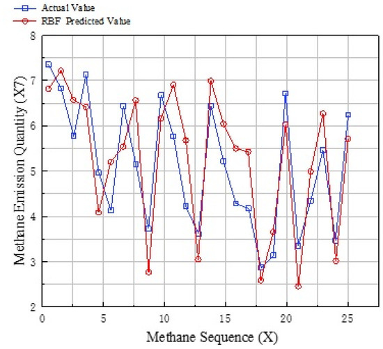
Figure 5.
Comparison between RBF the neural network model predicted value and actual value.
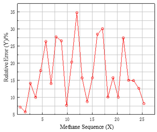
Figure 6.
RBF neural network model relative error.
3.2. Grey RBF Neural Network Model Prediction
The grey RBF neural network model combines the GM (1,1) model with the RBF neural network model. The input layer and the output layer are six and two neuron nodes, respectively. The modeling and prediction steps are as follows:
- (1)
- The first 275 sets of training samples accumulate to generate a sequence , which is used as the input vector of the RBF neural network model;
- (2)
- The first 275 sets of training samples are calculated using the GM (1,1) model to obtain , and use as the target vectors of the RBF neural network model;
- (3)
- Input the input vector and the target vector into the RBF neural network model to learn and train;
- (4)
- A cumulative operation of the last 25 sets of prediction samples to obtain the generated sequence;
- (5)
- The generated sequence in (4) is input into the RBF neural network model that has been trained, and the output values are: ;
- (6)
- Subtraction: , is the final predicted value;
- (7)
- Find the relative error.
Figure 7 is the comparison between the predicted value and the actual value of the grey RBF neural network model, and Figure 8 is the relative error of the model.
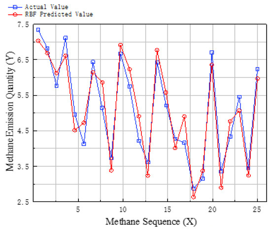
Figure 7.
Comparison between grey RBF neural network model predicted value and actual value.
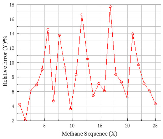
Figure 8.
Grey RBF neural network model relative error.
3.3. Improved Grey RBF Neural Network Model Prediction
Follow the steps to build an improved grey RBF neural network model and make predictions. The modeling and prediction steps are as follows:
- (1)
- The first 275 groups of training samples are log processed to obtain the corresponding number series . Logarithmic processing of the last 25 groups of prediction samples yields , where of the last 25 groups does not perform logarithmic processing;
- (2)
- The sequence obtained by the first 275 logarithmic processing in (1) is used to accumulate a generated sequence , which is used as the input vector of the improved RBF neural network model;
- (3)
- Then we can bring , which is Obtained by logarithmic processing before 275 groups in step (1), into GM(1,1) and calculate . is the target vector of the improved RBF neural network model;
- (4)
- A cumulative operation is performed on the obtained by the last 25 groups of logarithmic processing to obtain a generated sequence ;
- (5)
- Input in (5) into the improved RBF neural network model with completed training, and the output value is: ;
- (6)
- Subtract: ;
- (7)
- Index reduction: , is the final predicted value;
- (8)
- Finding the relative error.
3.4. Analysis and Comparison of Prediction Results of Three Models
We compared the relative errors of the above three models, as shown in Figure 9.
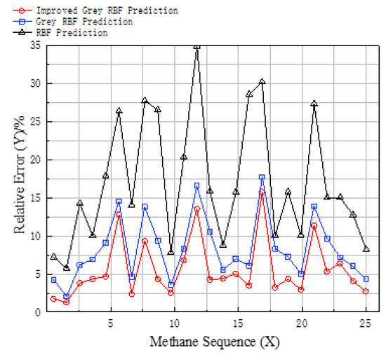
Figure 9.
Relative errors of three models.
As can be seen from Figure 9, the relative errors of the RBF neural network model, the grey RBF neural network model, and the improved grey RBF neural network model become smaller in order, and the model’s prediction accuracy improves in turn, indicating the grey GM (1,1) weakens the randomness of the sample, which improves the prediction accuracy of the grey RBF neural network model. Compared with the grey RBF neural network model, the advantages of the improved GM (1,1) model and the improved RBF neural network model are the following two aspects. On the one hand, the sample data becomes smoother, which further weakens the sample randomness. On the other hand, the RBF neural network model has been improved, and the model performance has been improved. Therefore, the improved grey RBF neural network model further improves the prediction accuracy. The average relative error of 25 groups is 5.63% for the improved grey RBF neural network model, 8.34% for the grey RBF neural network model, and 17.08% for the RBF neural network model, respectively. Among the three models, the improved grey RBF neural network model has the highest prediction accuracy.
4. Conclusions
Combining conventional neural network and grey theory, an improved grey RBF neural network model for methane emission prediction is proposed. The main conclusions are as follows:
- The RBF neural network model has the lowest accuracy, followed by the grey RBF neural network model, and the improved grey RBF neural network model has the highest accuracy. The grey RBF neural network model improves the accuracy of the model by weakening the randomness of the sample. The improved grey RBF neural network model has further improved both in terms of weakening the randomness of sample data and the performance of the network model itself.
- The average relative error of 25 groups is 5.63% for the improved grey RBF neural network model, 8.34% for the grey RBF neural network model, and 17.08% for the RBF neural network model, respectively. The relative error of the improved grey RBF neural network model is mostly within 5%, and the other few are basically within 10%, which gives an ideal prediction effect.
- The methane emission prediction model in this work only considers seven factors that affect gas emission, namely, coal seam depth, coal seam thickness, coal seam methane content, coal seam spacing, daily progress, daily output, and methane emission, respectively. In addition, factors, such as geological structure, physical and mechanical properties of coal pillars, working face width, support pressure, and other factors all affect methane emissions. In order to make the results of the prediction model more reliable, it is necessary to consider more comprehensive factors. At the same time, it is necessary to collect more in-situ data and provide enough training samples for the prediction model.
- At present, both grey theory and neural network have their own limitations in methane emission. How to improve the shortcomings of the two is a problem that needs to be solved urgently in the future. In addition, how to make the performance of the grey neural network model be more fully exerted in the combination of grey theory and neural network still needs further research. All of the above restrict the performance of the grey neural network model, which needs to be further studied and resolved in the future.
Author Contributions
Conceptualization, Y.Y. and C.W.; methodology, Y.Y.; software, Q.D.; validation, Q.D., Y.B. and Y.Y.; formal analysis, Q.D.; investigation, Y.Y.; resources, Y.Y.; data curation, Q.D.; writing—original draft preparation, Q.D.; writing—review and editing, Y.Y. and C.W.; visualization, Y.Y.; supervision, Y.Y. All authors have read and agreed to the published version of the manuscript.
Funding
This work was supported by the National Natural Science Foundation of China (Grant No. 51404167); Shanxi Scholarship Council of China (HGKY2019038); Natural Science Foundation of Shanxi Province (Grant No. 201801D121034; Natural Science Foundation of Shanxi Province (Grant No. 201901D211066); Shanxi Provincial Key R&D Project (Grant No. 201803D31051); Shanxi Soft Science Research Project (Grant No. 201803D31051); China postdoctoral science foundation funding project (Grant No. 2016M590151).
Acknowledgments
The author thanks the scholars who helped in the writing of the paper, and the editors and reviewers for their work during the publication of the paper.
Conflicts of Interest
The authors declare no conflict of interest.
Data Availability
The article data used to support the findings of this study are included within the article.
References
- Burgherr, P.; Hirschberg, S. Assessment of severe accident risks in the Chinese coal chain. Int. J. Risk Assess. Manag. 2007, 7, 1157–1175. [Google Scholar] [CrossRef]
- Geng, F.; Saleh, J.H. Challenging the emerging narrative: Critical examination of coalmining safety in China, and recommendations for tackling mining hazards. Saf. Sci. 2015, 75, 36–48. [Google Scholar] [CrossRef]
- Tong, R.; Yang, Y.; Ma, X.; Zhang, Y.; Li, S.; Yang, H. Risk Assessment of Miners’ Unsafe Behaviors: A Case Study of Gas Explosion Accidents in Coal Mine, China. Int. J. Environ. Res. Public Health 2019, 16, 1765. [Google Scholar] [CrossRef]
- Liu, D.; Xiao, X.; Li, H.; Wang, W. Historical evolution and benefit–cost explanation of periodical fluctuation in coal mine safety supervision: An evolutionary game analysis framework. Eur. J. Oper. Res. 2015, 243, 974–984. [Google Scholar] [CrossRef]
- Zhou, X.; Jiang, M.-X. Statistical Analysis and Safety Management on China’s Coal Mine Gas Accident from 2006 to 2015. IETI Trans. Bus. Manag. Sci. 2016, 1, 29–38. [Google Scholar]
- Myhre, G.; Shindell, D.; Bréon, F.-M.; Collins, W.; Fuglestvedt, J.; Huang, J.; Koch, D.; Lamarque, J.-F.; Lee, D.; Mendoza, B.; et al. Anthropogenic and natural radiative forcing. In Climate Change 2013: The Physical Science Basis. Contribution of Working Group I to the Fifth Assessment Report of the Intergovernmental Panel on Climate Change; Stocker, T.F., Qin, D., Plattner, G.-K., Tignor, M., Allen, S.K., Doschung, J., Nauels, A., Xia, Y., Bex, V., Midgley, P.M., Eds.; Cambridge University Press: Cambridge, UK, 2013; pp. 659–740. [Google Scholar]
- Balcombe, P.; Speirs, J.F.; Brandon, N.P.; Hawkes, A.D. Methane emissions: Choosing the right climate metric and time horizon. Environ. Sci. Processes Impacts 2018, 20, 1323–1339. [Google Scholar] [CrossRef]
- Crow, D.J.G.; Balcombe, P.; Brandon, N.; Hawkes, A.D. Assessing the impact of future greenhouse methane emissions from natural gas production. Sci. Total Environ. 2019, 668, 1242–1258. [Google Scholar] [CrossRef]
- Warmuzinski, K. Harnessing methane emissions from coal mining. Process Saf. Environ. Prot. 2008, 86, 315–320. [Google Scholar] [CrossRef]
- Shi, S.; Han, J.; Wu, J.; Li, H.; Worrall, R.; Hua, G.; Xin, S.; Liu, W. Fugitive coal mine methane emissions at five mining areas in China. Atmos. Environ. 2011, 45, 2220–2232. [Google Scholar]
- Cheng, Y.-P.; Wang, L.; Zhang, X.-L. Environmental impact of coal mine methane emissions and responding strategies in China. Int. J. Greenh. Gas Control 2011, 5, 157–166. [Google Scholar] [CrossRef]
- Brodny, J.; Tutak, M. Analysis of methane emission into the atmosphere as a result of mining activity. In Proceedings of the International Multidisciplinary Scientific GeoConference: SGEM, Albena, Bulgaria, 30 June–6 July 2016; pp. 83–90. [Google Scholar]
- Setiawan, A.; Kennedy, E.M.; Stockenhuber, M. Development of Combustion Technology for Methane Emitted from Coal-Mine Ventilation Air Systems. Energy Technol. 2017, 5, 521–538. [Google Scholar] [CrossRef]
- Sun, H.; Cao, J.; Li, M.; Zhao, X.; Dai, L.; Sun, D.; Wang, B.; Zhai, B. Experimental Research on the Impactive Dynamic Effect of Gas-Pulverized Coal of Coal and Gas Outburst. Energies 2018, 11, 797. [Google Scholar] [CrossRef]
- Li, Z.; Wang, E.; Ou, J.; Liu, Z. Hazard evaluation of coal and gas outbursts in a coal-mine roadway based on logistic regression model. Int. J. Rock Mech. Min. Sci. 2015, 80, 185–195. [Google Scholar] [CrossRef]
- Zhou, H.; Yang, Q.; Cheng, Y.; Ge, C.; Chen, J. Methane drainage and utilization in coal mines with strong coal and gas outburst dangers: A case study in Luling mine, China. J. Nat. Gas Sci. Eng. 2014, 20, 357–365. [Google Scholar] [CrossRef]
- National Coal Mine Safety Administration. Available online: http://www.chinacoal-safety.gov.cn/gk/sgcc/ (accessed on 1 July 2020).
- Zhang, J.; David, C.; Xu, K.; You, G. Focusing on the patterns and characteristics of extraordinarily severe gas explosion accidents in Chinese coal mines. Process Saf. Environ. Prot. 2018, 117, 390–398. [Google Scholar] [CrossRef]
- Tutak, M.; Brodny, J. Forecasting Methane Emissions from Hard Coal Mines Including the Methane Drainage Process. Energies 2019, 12, 3840. [Google Scholar] [CrossRef]
- Karacan, C.Ö.; Ruiz, F.A.; Cotè, M.; Phipps, S. Coal mine methane: A review of capture and utilization practices with benefits to mining safety and to greenhouse gas reduction. Int. J. Coal Geol. 2011, 86, 121–156. [Google Scholar] [CrossRef]
- Yang, X.; Liu, Y.; Li, Z.; Zhang, C.; Xing, Y. Vacuum Exhaust Process in Pilot-Scale Vacuum Pressure Swing Adsorption for Coal Mine Ventilation Air Methane Enrichment. Energies 2018, 11, 1030. [Google Scholar] [CrossRef]
- Ju, Y.; Li, X. New research progress on the ultrastructure of tectonically deformed coals. Prog. Nat. Sci. 2009, 19, 1455–1466. [Google Scholar] [CrossRef]
- Zhang, B.; Chen, G.Q. Methane emissions by Chinese economy: Inventory and embodiment analysis. Energy Policy 2010, 38, 4304–4316. [Google Scholar] [CrossRef]
- Zhang, B.; Chen, G.Q.; Li, J.S.; Tao, L. Methane emissions of energy activities in China 1980–2007. Renew. Sustain. Energy Rev. 2014, 29, 11–21. [Google Scholar] [CrossRef]
- Li, W.; Younger, P.L.; Cheng, Y.; Zhang, B.; Zhou, H.; Liu, Q.; Dai, T.; Kong, S.; Jin, K.; Yang, Q. Addressing the CO2 emissions of the world’s largest coal producer and consumer: Lessons from the Haishiwan Coalfield, China. Energy 2015, 80, 400–413. [Google Scholar] [CrossRef]
- Liu, Y.; Wang, F.; Tang, H.; Liang, S. Well type and pattern optimization method based on fine numerical simulation in coal-bed methane reservoir. Environ. Earth Sci. 2015, 73, 5877–5890. [Google Scholar] [CrossRef]
- Guo, P.; Cheng, Y.; Jin, K.; Liu, Y. The impact of faults on the occurrence of coal bed methane in Renlou coal mine, Huaibei coalfield, China. J. Nat. Gas Sci. Eng. 2014, 17, 151–158. [Google Scholar] [CrossRef]
- Liu, S.; Xie, L.; Zhang, S. Synchronization of a class of nonlinear network flow systems. Int. J. Robust. Nonlinear Control 2016, 26, 565–577. [Google Scholar] [CrossRef]
- He, X.; Song, L. Status and future tasks of coal mining safety in China. Saf. Sci. 2012, 50, 894–898. [Google Scholar] [CrossRef]
- Jing, G.-X.; Xu, S.-M.; Heng, X.-W.; Li, C.-Q. Research on the Prediction of Methane emission Quantity in Coal Mine Based on Grey System and Linear Regression for One Element. Procedia Eng. 2011, 26, 1585–1590. [Google Scholar]
- Mishra, D.P.; Kumar, P.; Panigrahi, D.C. Dispersion of methane in tailgate of a retreating longwall mine: A computational fluid dynamics study. Environ. Earth Sci. 2016, 75, 475. [Google Scholar] [CrossRef]
- Noack, K. Control of methane emissions in underground coal mines. Int. J. Coal Geol. 1998, 35, 57–82. [Google Scholar] [CrossRef]
- Dong, D. Mine Methane emission Prediction based on Gaussian Process Model. Procedia Eng. 2012, 45, 334–338. [Google Scholar] [CrossRef]
- Cheng, L.; Li, S.; Yang, S. Methane emission quantity prediction and drainage technology of steeply inclined and extremely thick coal seams. Int. J. Min. Sci. Technol. 2018, 28, 415–422. [Google Scholar] [CrossRef]
- Booth, P.; Brown, H.; Nemcik, J.; Ting, R. Spatial context in the calculation of methane emissions for underground coal mines. Int. J. Min. Sci. Technol. 2017, 27, 787–794. [Google Scholar] [CrossRef]
- Wei, C.; Xu, M.; Sun, J.; Li, X.; Ji, C. Coal Mine Methane emission Grey Dynamic Prediction. Procedia Eng. 2011, 26, 1157–1167. [Google Scholar]


Publisher’s Note: MDPI stays neutral with regard to jurisdictional claims in published maps and institutional affiliations. |
© 2020 by the authors. Licensee MDPI, Basel, Switzerland. This article is an open access article distributed under the terms and conditions of the Creative Commons Attribution (CC BY) license (http://creativecommons.org/licenses/by/4.0/).