Real-Time Multiparameter Identification of a Salient-Pole PMSM Based on Two Steady States

Abstract

Real-time multiparameter identification has been widely investigated in relation to high-performance control and fault diagnosis of salient-pole permanent magnet synchronous motors (PMSMs). However, it is rank-deficient for simultaneously estimating flux, resistance, and dq-axis inductances based on one steady state under maximum torque per ampere (MTPA) control, which will cause the ill-convergence problem in the results. This paper proposes a new method to solve the rank deficiency problem in the multiparameter identification of salient-pole PMSMs in systems where the motor working conditions do not change frequently. For this type of system, a second steady state is constructed in order to meet the full-rank conditions for multiparameter identification and minimize the torque ripple. Furthermore, in order to reduce the influence of inductance variations, a better shift direction from the first steady state to the second is ensured based on the analysis of the theoretical error. Simulation and experimental results show that the proposed method demonstrates good identification performance.

1. Introduction

Permanent magnet synchronous motors (PMSMs) are now widely employed in rail transit vehicles, industrial servo drives and other domains because of their high efficiency, power factor and power density. It is important to obtain accurate parameters for high-performance control and fault diagnosis. In particular, maximum torque per ampere (MTPA) control, which is based on motor parameters such as flux and dq-axis inductances, is the most common method to maximize the efficiency of the system. Therefore, accurate flux and dq-axis inductances are essential to ensure the accuracy of system output under MTPA control. However, these parameters are affected by temperature and operating conditions. Flux and resistance are mainly affected by temperature [1], while inductances are mainly affected by the current [2]. Hence, many methods have been proposed to estimate the inductance and calculate the flux linkage of PMSMs.

Offline parameter identification methods for PMSMs are mainly used for the initial setting of motor parameters. For example, a step input signal was injected to calculate the flux and identify the inductances in [3,4]. In [5], the fundamental components of phase voltages and currents are acquired by fast Fourier transform (FFT) in order to identify the inductance. This type of method can identify relatively accurate motor parameters, but the identification process often requires complex data acquisition and fails to reflect the variation of parameters caused by temperature differences.

Numerous studies have focused on real-time parameter identification [6,7,8,9,10,11,12,13]. In [6], resistance and inductance were identified by fixing the flux to a nominal value. In [7], a d-axis current injection method was used to identify the resistance and flux for the first time. The method in [8] achieved good results in resistance and flux identification, but failed to identify the inductance. In [9], a recursive least squares (RLS) algorithm was proposed to identify the flux and dq-axis inductances. In [10], an extended Kalman filter (EKF) was employed to identify the resistance and flux. This type of method is mostly based on steady-state voltage equations. However, it is rank-deficient to identify more than two parameters using one set of steady-state equations, and the results are greatly influenced by inaccurate nominal or initial parameters. In [9,11], the authors proposed that injecting a signal into a d-axis current could solve the rank deficiency problem in multiparameter identification, but this resulted in nonnegligible perturbation in the torque. In addition to the proposals in these studies, other methods were introduced in [12,13] which used a sinusoidal d-axis current injection based on dynamic equations, but this resulted in torque ripple during identification.

In this paper, a novel and simple method is proposed for real-time multiparameter identification of salient-pole PMSMs, especially in systems where the motor working conditions do not change frequently, such as rail transit systems. During the steady state operation process of the motor, a temporary steady state is designed for the simultaneous estimation of flux, resistance and dq-axis inductances. The torque ripple during the state transition process is so negligible that it has little effect on the speed control system, especially in a rail transit system with large inertia. In addition, the error caused by the variation of inductances is analyzed, and the better shift direction of the state transition process is calculated. The use of mean sampling instead of RLS means that there are no complicated matrix calculations in this algorithm. Thus, the identification process is very simple and needs minimal computation compared with other methods. Simulation and experimental results validate the good performance of the proposed method.

2. Implementation of Multiparameter Identification of a Salient-Pole PMSM

2.1. Full-Rank Matrix of a Salient-Pole PMSM

The steady-state voltage equations of a salient-pole PMSM in a rotating frame are given by

$$\{\begin{array}{l}{u}_d=R_s{i}_d-{\omega }_e{L}_q{i}_q\hfill \\ u_q=R_s{i}_q+{\omega }_e{L}_d{i}_d+{\omega }_e{\psi }_f\hfill \end{array}$$

(1)

where u_d, u_q, i_d and i_q are the dq-axis voltages and currents, respectively; R_s is the stator resistance; L_d and L_q are the machine dq-axis inductances; ψ_f is the rotor flux linkage; and ω_e is the electrical angular speed. If the rank of Equation (1) is less than the number of parameters (ψ_f, R_s, L_d, L_q) to be identified, the equations are rank-deficient. Therefore, it is impossible to identify four parameters with one set of steady-state equations [9,11].

In order to solve the rank deficiency problem of multiparameter identification, a temporary steady state which is not linearly dependent on the normal steady state can be constructed. Based on Equation (1), the new fourth-order equations shown in Equation (2) can be obtained.

$$\{\begin{array}{l}{u}_{d1}=R_s{i}_{d1}-{\omega }_{e1}{L}_q{i}_{q1}\hfill \\ \begin{array}{l}{u}_{q1}=R_s{i}_{q1}+{\omega }_{e1}{L}_d{i}_{d1}+{\omega }_{e1}{\psi }_f\\ u_{d2}=R_s{i}_{d2}-{\omega }_{e2}{L}_q{i}_{q2}\\ u_{q2}=R_s{i}_{q2}+{\omega }_{e2}{L}_d{i}_{d2}+{\omega }_{e2}{\psi }_f\end{array}\hfill \end{array}$$

(2)

where the subscript 1 denotes the normal steady state of the motor working under MTPA control and the state that multiparameter identification should take, and the subscript 2 denotes the artificial temporary steady state, which is intended to meet the full-rank condition and so on.

Since the process of parameter identification is very short, the speed of these two operation points can be considered as constant ω_e. Then, Equation (2) can be rewritten into a matrix format as

$$\left[\begin{array}{c}{u}_{d1}\\ u_{q1}\\ u_{d2}\\ u_{q2}\end{array}\right]=\left[\begin{array}{cccc}{i}_{d1}& 0& -{\omega }_e{i}_{q1}& 0\\ i_{q1}& {\omega }_e{i}_{d1}& 0& {\omega }_e\\ i_{d2}& 0& -{\omega }_e{i}_{q2}& 0\\ i_{q2}& {\omega }_e{i}_{d2}& 0& {\omega }_e\end{array}\right]\left[\begin{array}{c}{R}_s\\ L_d\\ L_q\\ {\psi }_f\end{array}\right]$$

(3)

or

$$Y_{4\times 1}=X_{4\times 4}{\mathsf{\theta }}_{4\times 1}$$

(4)

where Y_4×1, X_4×4 and θ_4×1 are the input voltage matrix, input coefficient matrix and output parameters matrix, respectively.

The condition that Equation (4) must have a unique solution can be met when X_4×4 is of full rank or its determinant is not equal to zero, as shown in Equation (5).

$$\left|X_{4\times 4}\right|={\omega }_e^3\left(i_{d1}{i}_{q2}-i_{q1}{i}_{d2}\right)\left(i_{d2}-i_{d1}\right)\ne 0$$

(5)

The following two conditions are obtained to satisfy Equation (5):

$$i_{d1}{i}_{q2}\ne i_{d2}{i}_{q1}$$

(6)

$$i_{d2}\ne i_{d1}$$

(7)

Equation (6) requires that these two operating points are not on the same straight line through the origin. Furthermore, Equation (7) requires that the d-axis current is appropriately changed.

In order to satisfy Equations (6) and (7), many papers propose to inject additional d-axis current into the machine [9,11]. However, a d-axis current injection method will result in negligible torque ripple during identification, according to Equation (8):

$$\Delta T_e=\frac{3}{2}{n}_p\left(L_d-L_q\right)\Delta i_d{i}_q$$

(8)

where ΔT_e is the torque ripple, n_p is the number of pole pairs in the motor and Δi_d is the injected d-axis current.

Taking the motor parameters from the later section as an example, Figure 1 shows the relationship between the amplitude of torque ripple and the amplitude of injected d-axis current when the q-axis current is the rated current. The torque ripple is about 40% of the rated torque when the amplitude of Δi_d is the rated current.

2.2. Construction of the Second Steady State

The above analysis shows that we can identify four parameters simultaneously by constructing a temporary steady state and combining it with the normal steady state. This section shows how to construct a temporary steady state without changing the output torque of the system.

In Figure 2, point ① is the intersection of the MTPA and constant torque curves under normal operation conditions. The values of the voltages, currents and speed are measured as u_d1, u_q1, i_d1, i_q1 and ω_e at the point when the motor reaches the first steady state. After that, the normal operating point ① shifts to the left/right to temporary operating point ② or ②′ along the constant torque curve for a short time. Similarly, when the motor reaches the second steady state, the values of the voltages, currents and speed are u_d2, u_q2, i_d2, i_q2 and ω_e. Finally, the temporary operating point ② or ②′ returns to the normal operating point ① along the original path. Compared with the d-axis current injection method, the proposed method presents a smaller perturbation in torque during identification, as shown in Figure 3. Note that, in this case, the proposed method satisfies both Equations (6) and (7) such that θ_4×1 in Equation (4) has a unique solution.

2.3. Mean Sampling Algorithm

In theory, according to Equation (3), only one data group needs to be sampled for each steady state when simultaneously estimating four parameters. However, single sampling can lead to huge errors in identification results because of nonideal factors. After multiple sampling, it is necessary to select an appropriate algorithm to identify the parameters. An RLS algorithm is often employed for parameter identification and has been explained in many papers, this paper only presents its special application with the proposed method. The condition of the minimum error is given in [14].

$${\mathsf{\theta }}_{4\times 1}^{\ast }={\left(X_{4m\times 4}^{\mathrm{T}}{X}_{4m\times 4}\right)}^{-1}{X}_{4m\times 4}^{\mathrm{T}}{Y}_{4m\times 1}$$

(9)

where the subscript m denotes the mth sampling point in each steady state and the superscript * denotes the result of the proposed method. Expand Equation (9) into Equation (10):

$$\begin{array}{ll}{\mathsf{\theta }}_{4\times 1}^{\ast }=& {\left(\left[\begin{array}{ccc}{X}_{4\times 4}^{\mathrm{T}}\left(1\right)& \cdots & X_{4\times 4}^{\mathrm{T}}\left(m\right)\end{array}\right]{\left[\begin{array}{ccc}{X}_{4\times 4}^{\mathrm{T}}\left(1\right)& \cdots & X_{4\times 4}^{\mathrm{T}}\left(m\right)\end{array}\right]}^{\mathrm{T}}\right)}^{-1}\\ & ·\left[\begin{array}{ccc}{X}_{4\times 4}^{\mathrm{T}}\left(1\right)& \cdots & X_{4\times 4}^{\mathrm{T}}\left(m\right)\end{array}\right]{\left[\begin{array}{ccc}{Y}_{4\times 1}^{\mathrm{T}}\left(1\right)& \cdots & Y_{4\times 1}^{\mathrm{T}}\left(m\right)\end{array}\right]}^{\mathrm{T}}\end{array}$$

(10)

The coefficient matrix X_4×4(1) = … = X_4×4(m) = X_4×4 when the current regulators perform well. Therefore, Equation (10) can be simplified as Equation (11):

$$\begin{array}{ll}{\mathsf{\theta }}_{4\times 1}^{\ast }& ={\left(m{X}_{4\times 4}^{\mathrm{T}}{X}_{4\times 4}\right)}^{-1}{X}_{4\times 4}^{\mathrm{T}}\left[Y_{4\times 1}\left(1\right)+\cdots +Y_{4\times 1}\left(m\right)\right]\\ & =X_{4\times 4}^{-1}\frac{\left[Y_{4\times 1}\left(1\right)+\cdots +Y_{4\times 1}\left(m\right)\right]}{m}=X_{4\times 4}^{-1}{\overline{Y}}_{4\times 1}\end{array}$$

(11)

where the superscript “−” denotes the mean sampling value.

According to Equation (11), the mean sampling algorithm, which is equivalent to an RLS algorithm since the coefficient matrix is held constant in this method, can be employed due to its smaller computation. Therefore, substituting the averages of the measured quantities into Equation (4) yields Equations (12)–(14):

$$\{\begin{array}{l}{\psi }_f^{\ast }=\frac{\left(i_{q2}{\overline{u}}_{d1}-i_{q1}{\overline{u}}_{d2}\right)+\left(i_{d2}{\overline{u}}_{q1}-i_{d1}{\overline{u}}_{q2}\right)}{{\omega }_e\Delta i_d}\hfill \\ R_s^{\ast }=\frac{i_{q1}{\overline{u}}_{d2}-i_{q2}{\overline{u}}_{d1}}{\Delta i_{dq}}\hfill \\ L_d^{\ast }=\frac{\Delta i_q\left(i_{q2}{\overline{u}}_{d1}-i_{q1}{\overline{u}}_{d2}\right)}{{\omega }_e\Delta i_{dq}\Delta i_d}+\frac{\left({\overline{u}}_{q2}-{\overline{u}}_{q1}\right)}{{\omega }_e\Delta i_d}\hfill \\ L_q^{\ast }=\frac{i_{d1}{\overline{u}}_{d2}-i_{d2}{\overline{u}}_{d1}}{{\omega }_e\Delta i_{dq}}\hfill \end{array}$$

(12)

or

$$\begin{array}{ll}{\mathsf{\theta }}_{4\times 1}^{\ast }& =X_{4\times 4}^{-1}{\overline{Y}}_{4\times 1}\\ & =\left[\begin{array}{cccc}-{\omega }_e{i}_{q2}\Delta i_d& 0& {\omega }_e{i}_{q1}\Delta i_d& 0\\ i_{q2}\Delta i_q& -\Delta i_{dq}& -i_{q1}\Delta i_q& \Delta i_{dq}\\ -i_{d2}\Delta i_d& 0& i_{d1}\Delta i_d& 0\\ i_{q2}\Delta i_{dq}& i_{d2}\Delta i_{dq}& -i_{q1}\Delta i_{dq}& -i_{d1}\Delta i_{dq}\end{array}\right]\frac{{\overline{Y}}_{4\times 1}}{{\omega }_e\Delta i_{dq}\Delta i_d}\end{array}$$

(13)

where

$$\{\begin{array}{l}\Delta i_d=i_{d2}-i_{d1}\hfill \\ \Delta i_{dq}=i_{d2}{i}_{q1}-i_{d1}{i}_{q2}\hfill \end{array}$$

(14)

The value of △i_d should be sufficiently high such that the effect of voltage errors on the identification result can be minimized. Finally, according to Equations (12)–(14), it is possible to simultaneously identify all four parameters using a simple algorithm rather than RLS or EKF, which contain complicated matrix calculations.

3. Error Analysis

3.1. Theoretical Error

The feasibility of the proposed method is analyzed in Section 2. The performance of the method is influenced by parameter variations, and analyzing the error caused by these variations can improve the accuracy of identification.

Since the interval between two steady states is short, the temperature can be considered not to change during the identification process. Therefore, the flux and resistance, which are mainly affected by temperature, can be assumed to be constant during identification. However, in practice, the inductance changes with the current. The inductances, which are set to be constant in the derivations of Equations (2)–(14), result in theoretical errors. In order to simplify the analysis, it is assumed that the dq-axis inductances can be denoted as a linear function of the dq-axis currents [15,16,17], as given below.

$$\{\begin{array}{c}{L}_{dx}=L_{d0}-\alpha i_{dx}\\ L_{qx}=L_{q0}-\beta i_{qx}\end{array}$$

(15)

where the subscript x denotes the xth steady state and the subscript 0 denotes the value at zero current. α and β are both positive values that stand for the self-saturation constants.

Substituting Equation (15) into Equation (2) yields Equation (16):

$$\{\begin{array}{l}{u}_{d1}=i_{d1}{R}_s-{\omega }_e{i}_{q1}{L}_{q0}+{\omega }_e{i}_{q1}^2\beta \hfill \\ u_{q1}=i_{q1}{R}_s+{\omega }_e{i}_{d1}{L}_{d0}-{\omega }_e{i}_{d1}^2\alpha +{\omega }_e{\psi }_f\hfill \\ u_{d2}=i_{d2}{R}_s-{\omega }_e{i}_{q2}{L}_{q0}+{\omega }_e{i}_{q2}^2\beta \hfill \\ u_{q2}=i_{q2}{R}_s+{\omega }_e{i}_{d2}{L}_{d0}-{\omega }_e{i}_{d2}^2\alpha +{\omega }_e{\psi }_f\hfill \end{array}$$

(16)

This can be simplified according to the original derivation process as

$$\left[\begin{array}{c}{R}_s^{\ast }\\ L_d^{\ast }\\ L_q^{\ast }\\ {\psi }_f^{\ast }\end{array}\right]=\left[\begin{array}{c}{R}_s\\ L_{d0}\\ L_{q0}\\ {\psi }_f\end{array}\right]+\frac{1}{\Delta i_{dq}\Delta i_d}\left[\begin{array}{c}{\omega }_e\beta i_{q1}{i}_{q2}\Delta i_d\Delta i_q\\ \alpha \Delta i_{dq}\left(i_{d1}^2-i_{d2}^2\right)-\beta i_{q1}{i}_{q2}\Delta i_q^2\\ \beta \Delta i_d\left(i_{d1}{i}_{q2}^2-i_{d2}{i}_{q1}^2\right)\\ \Delta i_{dq}\left(\alpha i_{d1}{i}_{d2}\Delta i_d-i_{q1}{i}_{q2}\beta \Delta i_q\right)\end{array}\right]$$

(17)

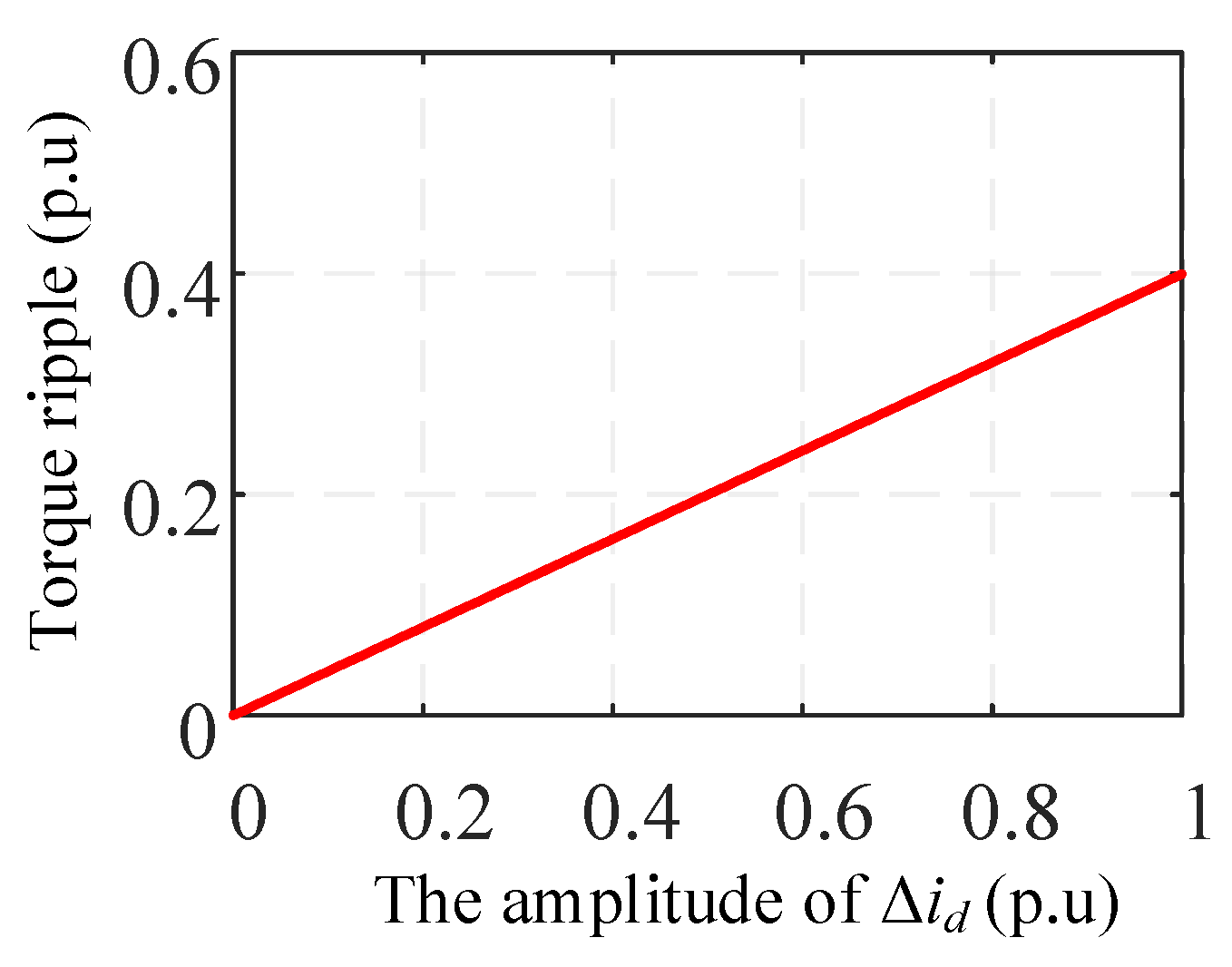
The theoretical error of the parameters in the first steady state is shown in (18):

$$\left[\begin{array}{c}{R}_{s1err}\\ L_{d1err}\\ L_{q1err}\\ {\psi }_{f1err}\end{array}\right]=\left[\begin{array}{c}{R}_s^{\ast }\\ L_d^{\ast }\\ L_q^{\ast }\\ {\psi }_f^{\ast }\end{array}\right]-\left[\begin{array}{c}{R}_s\\ L_{d0}-\alpha i_{d1}\\ L_{q0}-\beta i_{q1}\\ {\psi }_f\end{array}\right]=\left[\begin{array}{c}\frac{{\omega }_e\beta i_{q1}{i}_{q2}\Delta i_q}{\Delta i_{dq}}\\ -\alpha i_{d2}-\frac{\beta i_{q1}{i}_{q2}\Delta i_q^2}{\Delta i_{dq}\Delta i_d}\\ \frac{\beta i_{d1}{i}_{q2}\Delta i_q}{\Delta i_{dq}}\\ \alpha i_{d1}{i}_{d2}-\frac{\beta i_{q1}{i}_{q2}\Delta i_q}{\Delta i_d}\end{array}\right]$$

(18)

Under the traction condition, i_q > 0, i_d < 0. △i_q, △i_d and △i_dq are of the same polarity. Therefore, it is easy to deduce that R_s1err > 0 and L_q1err < 0, and that L_d1err and ψ_f1err are determined by the relative size between α and β. Among these values, only R_s1err is positively related to speed.

3.2. Influence of Torque Variation on Theoretical Error

According to Equation (18), it can be known that the theoretical error is quite complex because it is related to i_d1, i_q1, i_d2 and i_q2. However, i_q1, i_d2 and i_q2 can all be expressed by i_d1. Therefore, in order to perform a qualitative analysis of theoretical error, Equation (18) needs to be simplified, and can be expressed by i_d1.

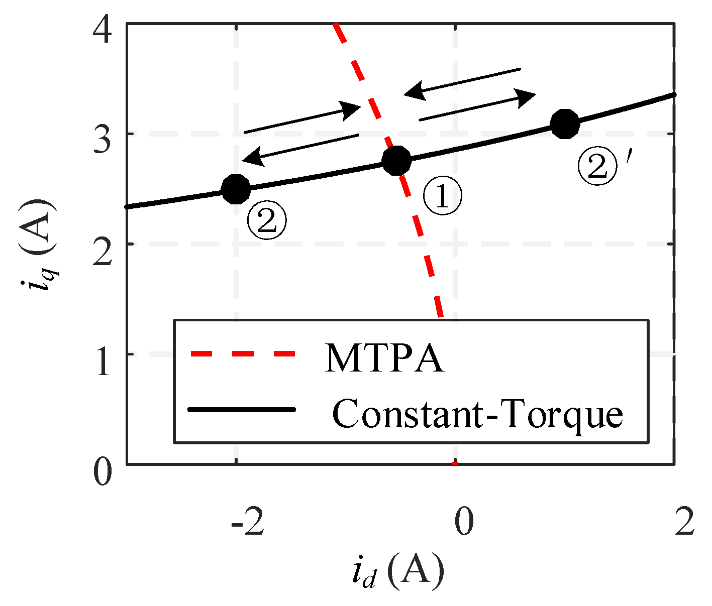
The constant torque curve in Figure 2 is given by

$$i_q=\frac{T_e^{\ast }}{1.5n_p\left[{\psi }_f+\left(L_d-L_q\right)i_d\right]}$$

(19)

Equation (19) can be expanded into a first-order Taylor expansion at i_d = 0 as

$$\begin{array}{ll}{i}_q& \approx \frac{\left(L_q-L_d\right)}{{\psi }_f}\frac{T_e^{\ast }}{1.5n_p{\psi }_f}{i}_d+\frac{T_e^{\ast }}{1.5n_p{\psi }_f}\\ & =c·b·i_d+b=k·i_d+b\end{array}$$

(20)

where k and b are positive coefficients including the motor parameters and torque command. They are both positively related to torque command. c is a positive value and is only related to the parameters.

The constant torque curve can be approximated as a straight line on which points (i_d1, i_q1) and (i_d2, i_q2) are located. Equation (21) can be obtained from Equation (20).

$$\{\begin{array}{l}\Delta i_q=i_{q2}-i_{q1}=k\Delta i_d\hfill \\ \Delta i_{dq}=i_{d2}{i}_{q1}-i_{d1}{i}_{q2}=b\Delta i_d\hfill \end{array}$$

(21)

The MTPA curve can be approximated as a straight line passing through the origin and perpendicular to the constant torque curve. The point (i_d1, i_q1) is located on this line such that Equation (22) can be obtained as

$$i_{q1}\approx -\frac{1}{k}{i}_{d1}=-\frac{1}{k}{f}_{MTPA}\left(T_e^{\ast }\right)$$

(22)

Therefore, i_q1, i_d2 and i_q2 can be expressed by i_d1 as Equation (23):

$$\{\begin{array}{l}{i}_{q1}=-i_{d1}/k\hfill \\ i_{d2}=i_{d1}+\Delta i_d\hfill \\ i_{q2}=k\left(i_{d1}+\Delta i_d\right)+b\hfill \end{array}$$

(23)

Substituting Equations (21) and (22) into Equation (19) yields Equation (24).

$$T_e^{\ast }\approx 1.5n_p{\psi }_f\sqrt{i_{d1}^2-\frac{i_{d1}}{c}}$$

(24)

The derivative of T*_ewith respect to i_d1 is given in

$$\frac{d{T}_e^{\ast }}{d{i}_{d1}}=\frac{3n_p{\psi }_f}{4}·\frac{2i_{d1}-\frac{i_{d1}}{c}}{\sqrt{i_{d1}^2-\frac{i_{d1}}{c}}}<0$$

(25)

Thus, T*_eis negatively related to i_d1. Substituting Equation (23) into Equation (18) yields Equation (26).

$$\left[\begin{array}{c}{R}_{s1err}\\ L_{d1err}\\ L_{q1err}\\ {\psi }_{f1err}\end{array}\right]=\left[\begin{array}{c}-{\omega }_e\beta i_{d1}\left(c{i}_{d1}+c\Delta i_d+1\right)\\ -\alpha \left(i_{d1}+\Delta i_d\right)+\beta cB\left(c{i}_{d1}+c\Delta i_d+1\right)\\ \beta cB\left(c{i}_{d1}+c\Delta i_d+1\right)\\ \alpha i_{d1}\left(i_{d1}+\Delta i_d\right)+\beta B\left(c{i}_{d1}+c\Delta i_d+1\right)\end{array}\right]$$

(26)

where

$$B=b{i}_{d1}=i_{d1}\sqrt{i_{d1}^2-\frac{i_{d1}}{c}}<0$$

(27)

In order to deduce the relationship between theoretical error and torque, the derivative of Equation (26) with respect to i_d1 is given in

$$\frac{d}{d{i}_{d1}}\left[\begin{array}{c}{R}_{s1err}\\ L_{d1err}\\ L_{q1err}\\ {\psi }_{f1err}\end{array}\right]=\left[\begin{array}{c}-{\omega }_e\beta \left(2c{i}_{d1}+c\Delta i_d+1\right)\\ -\alpha +\beta c\left[B^{\prime }\left(c{i}_{d1}+c\Delta i_d+1\right)+cB\right]\\ \beta c\left[B^{\prime }\left(c{i}_{d1}+c\Delta i_d+1\right)+cB\right]\\ 2\alpha i_{d1}+\alpha \Delta i_d+\beta \left[B^{\prime }\left(c{i}_{d1}+c\Delta i_d+1\right)+cB\right]\end{array}\right]$$

(28)

where

$$B^{\prime }={\left(i_{d1}\sqrt{i_{d1}^2-\frac{i_{d1}}{c}}\right)}^{\prime }=\frac{1}{\sqrt{i_{d1}^2-\frac{i_{d1}}{c}}}\left(2i_{d1}^2-\frac{3i_{d1}}{2c}\right)$$

(29)

Coefficient c is much less than 1 because the reluctance torque is much less than the synchronous torque in PMSMs. Thus, there exist the following relationships in Equation (28).

$$\{\begin{array}{l}2c{i}_{d1}+c\Delta i_d+1>0\hfill \\ B^{\prime }\left(c{i}_{d1}+c\Delta i_d+1\right)+cB\approx 1.5\sqrt{\frac{-i_{d1}}{c}}>0\hfill \end{array}$$

(30)

It is easy to deduce that dR_s1err/di_d1 < 0 and dL_q1err/di_d1 > 0. L_d1err and ψ_f1err should be derived in more detail. L_d1err is positively related to i_d1 when α and β satisfy Equation (31). ψ_f1err is positively related to i_d1 when α and β satisfy Equation (32).

$$\frac{\alpha }{\beta }<\frac{3}{2}k$$

(31)

$$\{\begin{array}{cc}\frac{\alpha }{\beta }<\frac{3b}{4bk-2\Delta i_d}\hfill & \hfill ,\Delta i_d<2bk\\ \frac{\alpha }{\beta }>0\hfill & \hfill ,\Delta i_d>2bk\end{array}$$

(32)

It can be verified that α is much smaller than β for the majority of PMSMs and that the motor described in this paper satisfies Equations (31) and (32). Therefore

$$\frac{d}{d{i}_{d1}}\left[\begin{array}{c}{R}_{s1err}\\ L_{d1err}\\ L_{q1err}\\ {\psi }_{f1err}\end{array}\right]=\left[\begin{array}{c}-\\ +\\ +\\ +\end{array}\right]$$

(33)

where − denotes a negative value and + denotes a positive value. Since di_d1/dT_e < 0, the conclusion is as follows:

$$\frac{d}{d{T}_e}\left[\begin{array}{c}{R}_{s1err}\\ L_{d1err}\\ L_{q1err}\\ {\psi }_{f1err}\end{array}\right]=\frac{d}{d{i}_{d1}}\left[\begin{array}{c}{R}_{s1err}\\ L_{d1err}\\ L_{q1err}\\ {\psi }_{f1err}\end{array}\right]·\frac{d{i}_{d1}}{d{T}_e}=\left[\begin{array}{c}+\\ -\\ -\\ -\end{array}\right]$$

(34)

In conclusion, only R_s1err is positively related to torque while the other values are negatively related to torque.

3.3. Comparison of Errors Due to the Left and Right Shifts

The shift direction of the operating point, which can be to the left or right, is analyzed here in order to minimize the theoretical error. Define △i_d = −I < 0 when the shift direction is left and △i_d = I > 0 when the shift direction is right. Substituting the different △i_d into Equation (26) and then subtracting the left shift error from the right shift error yields Equation (35)

$${\left[\begin{array}{c}{R}_{s1err}\\ L_{d1err}\\ L_{q1err}\\ {\psi }_{f1err}\end{array}\right]}_{right}-{\left[\begin{array}{c}{R}_{s1err}\\ L_{d1err}\\ L_{q1err}\\ {\psi }_{f1err}\end{array}\right]}_{left}=2\left[\begin{array}{c}-{\omega }_e\beta i_{d1}cI\\ \left(-\alpha +\beta c^{2}B\right)I\\ \beta c^{2}BI\\ \left(\alpha i_{d1}+\beta cB\right)I\end{array}\right]=\left[\begin{array}{c}+\\ -\\ -\\ -\end{array}\right]$$

(35)

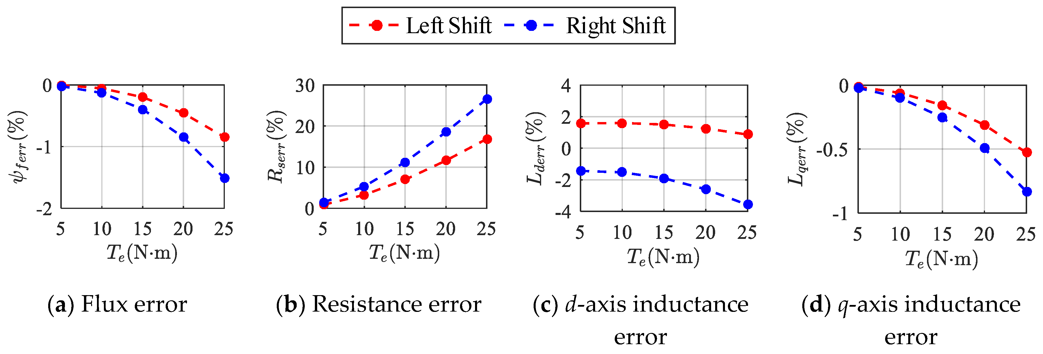
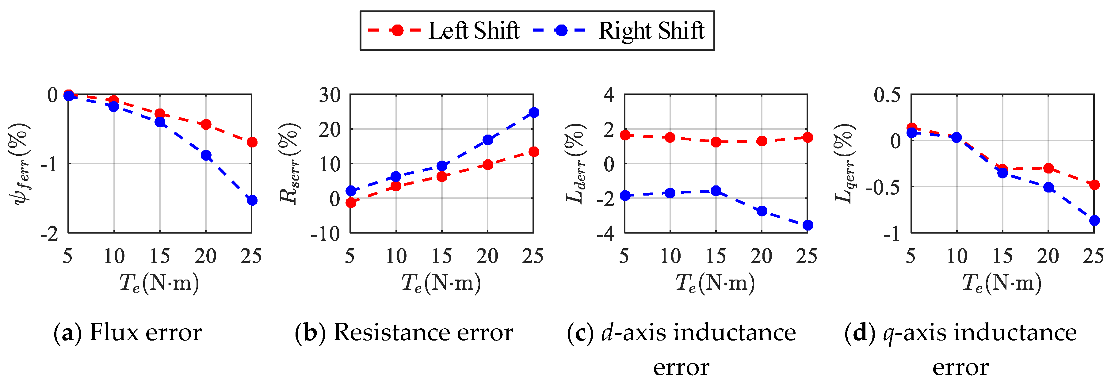
In order to analyze Equation (35) more intuitively, by combining it with the conclusion discussed above, we can plot the curves of the errors with increasing torque at 40 Hz, as shown in Figure 4. The percentage of the relative error is defined with reference to the reference parameter, as shown below

$$P_{err}(\%)=\frac{P^{\ast }-P_{ref}}{P_{ref}}\times 100\%$$

(36)

As can be seen from Figure 4, it is obvious that only R_s1err increases with increasing torque, while the other values show the opposite tendency. Furthermore, the right shift curve of R_s1err is always above the left shift curve, while the other values again show the opposite. In short, the magnitude of the left shift error is always smaller than the right one. For the braking condition, the same conclusion can also be obtained. In this case, it is recommended to identify parameters using left shift mode. Although R_s1err is quite large, its influence on torque control performance is usually so small that it can be ignored.

4. Simulation and Experimental Results of the Proposed Method

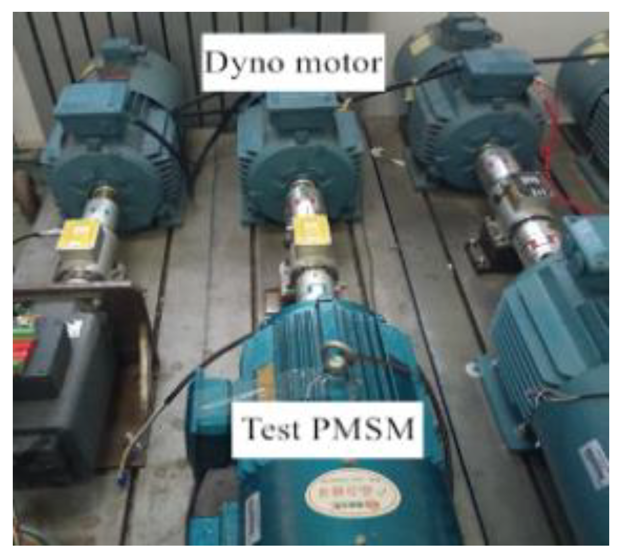
The proposed multiparameter identification method was verified through the simulation and experimental platforms of a 3 kW salient-pole PMSM. The experimental platform was as shown in Figure 5. The DSP(TMS320F28335)-based vector control system was employed to implement the proposed method.

In order to reduce the influence of nonideal factors such as initial position angle error, control delay and dead zones, we first had to compensate these factors in the experiment.

Considering the variability of the inductances, the second step was to obtain accurate reference parameters for the PMSM using offline measurement methods. For instance, L_d (L_q) was measured under the condition of different i_d (i_q) while i_q (i_d) = 0. The results are shown in

Table 1. PMSM test parameters.

Parameter	Value	Symbol
Rated power	3	kW
Rated current	5.12	A
Rated speed	750	rpm
Rated torque	25	N·m
Number of pole pairs	4
Flux	0.875	Wb
Resistance	2.58	Ω
d-axis inductance	26.7 − 0.2·id	mH
q-axis inductance	95.58 − 2.0·iq	mH

.

4.1. Simulation Results for Left and Right Shifts of the Operating Point with Different Torques

For the simulation, the proposed method was validated on a test motor operating at 40 Hz with load torques of 5, 10, 15, 20 and 25 N·m, respectively. The value of the △i_d was ±2 A. Nonideal factors such as temperature change and inverter nonlinearity were not considered in the simulation.

Figure 6 shows the simulation results of all four parameters. They are exactly the same as the theoretical results because the simulation environment was largely ideal. Therefore, the simulation verified the accuracy of the above theoretical analysis.

4.2. Experimental Results for Left and Right Shifts of the Operating Point with Different Torques

The experimental conditions were the same as those of the simulation except that there were nonideal factors that were difficult to compensate in the experiment, such as temperature, switching delay and switch voltage drop [18,19].

Figure 7 shows the experimental results for all four parameters. There are similarities between experimental results and the simulation results. For example, the variation trend of the parameter error was similar when the torque was more than 10 N·m. However, there were also large differences when the torque was 5 and 10 N·m because the pressure drop on parameters such as (ω_eL_di_d) was not large enough compared to the voltage errors caused by nonideal factors. The smaller the torque, the smaller the currents, and the greater the influence of voltage errors on the identification result, according to the voltage equations.

The resistance error, which reached between −20% and 30%, was the largest of the four parameter errors and was quite different from the simulation result. The reason is that the identification equation for resistance can be approximated as △u_d/△i_d, and therefore resistance is more sensitive to voltage errors. If there is a 0.5 V voltage error, the resulting identification of resistance error is 10%. Apart from this, the errors for the other parameters, which were kept within 5%, met the accuracy requirements for vector control.

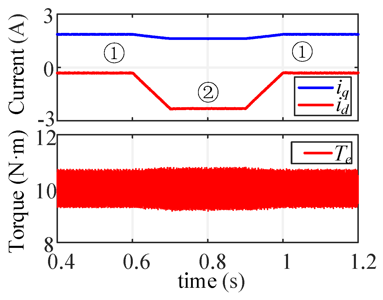
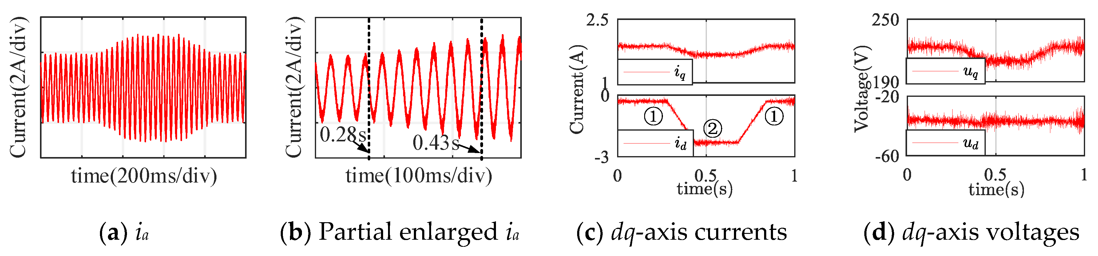
Figure 8 shows the waveforms of currents and voltages with a load torque of 10 N·m using left shift mode. The motor worked in the first steady state up to 0.28 s. The operating point moved left from 0.28 to 0.43 s and reached the second steady state at 0.43 s. During this period, the amplitude of i_a increased uniformly. The temporary operating point returned to the normal operating point along the original path from 0.68 to 0.83 s and reached the original steady state at 0.83 s. The dq-axis voltages contained a certain degree of higher harmonics.

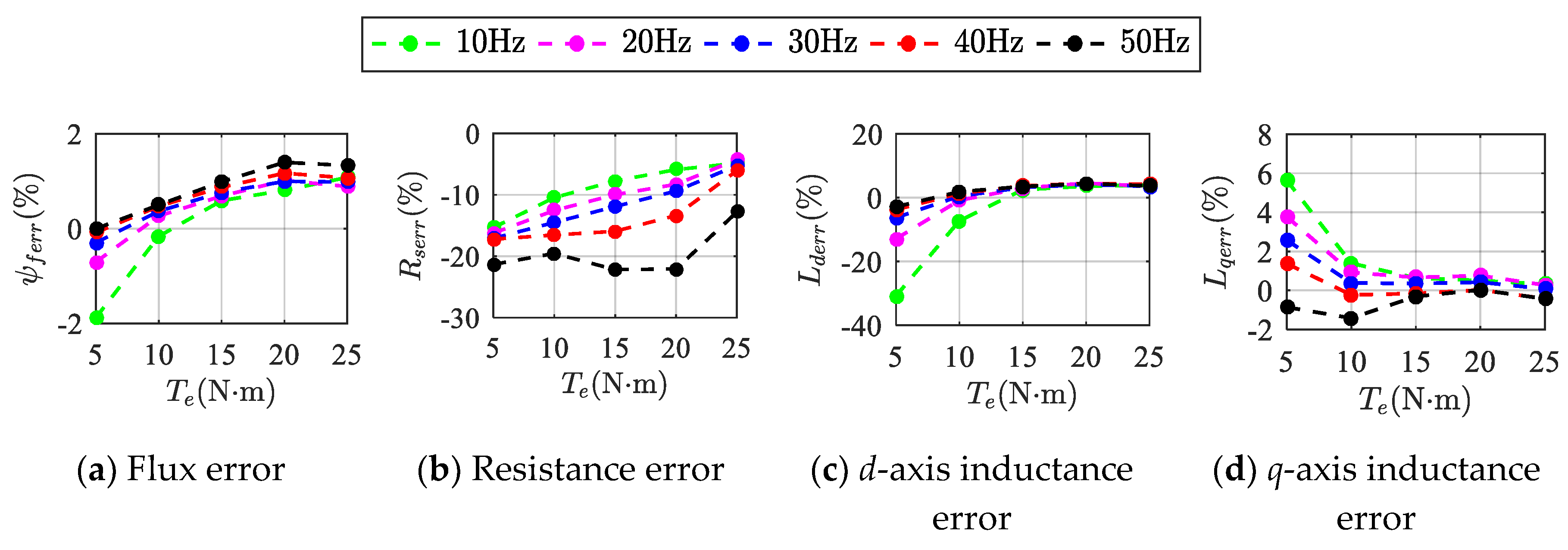
4.3. Experimental Results for Different Speeds

Figure 9 shows the experimental results for different speeds using left shift mode. The magnitude of R_s1err increased with increasing speed. One reason has already been mentioned above. The identification equation of R_s can be approximated as △u_d/△i_d, which is not related to speed. However, the voltage errors, which were caused by nonideal factors and related to speed, resulted in increasing R_s1err. Other errors, which were inversely proportional to the rotor speed according to Equation (12), decreased with increasing speed. L_d1err was about −30% with a load torque of 5 N·m at 10 Hz because the voltage due to L_d (ω_eL_di_d) was much smaller than that of ψ_f (ω_eψ_f) in the q-axis voltage equation. Thus, L_d was more sensitive to the voltage error than ψ_f. In conclusion, the higher the speed, the more accurate the identification will be.

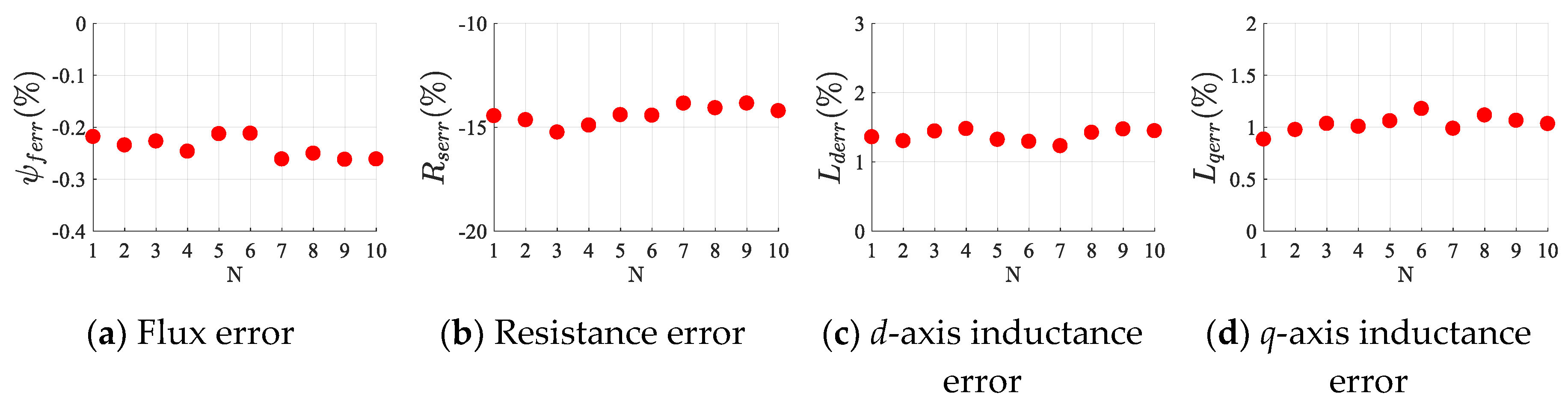
4.4. Identification Results with Inaccurate Initial Parameters

For the purpose of verifying the influence of inaccurate initial parameters on this method, the initial parameters of the motor, with reference to the reference parameters, were set according to Equation (37). Simultaneously, the identified parameters were applied to the vector control system. The algorithm was executed ten times with a load torque of 10 N·m at 40 Hz. The results are shown in Figure 10.

$$\{\begin{array}{l}{\psi }_f^{ini}=\left(0.8~1.2\right)·{\psi }_f\hfill \\ L_d^{ini}=\left(0.6~1.4\right)·L_d\hfill \\ L_q^{ini}=\left(0.4~1.6\right)·L_q\hfill \end{array}$$

(37)

The experimental results indicate that the inaccuracy of the initial parameters had no effect on this identification method. The reason for this is that the existence of the Proportion-Integral (PI) regulator kept the voltage constant at the steady state. Therefore, the identification result, which is based on the voltage, could be approximated as a constant value.

5. Conclusions

In this paper, a novel and simple method was designed for the real-time multiparameter identification of salient-pole PMSMs. Based on the steady-state equations of a salient-pole PMSM, a second steady state was constructed to meet full-rank conditions and minimize the torque ripple. The proposed error analysis method is applicable to the linear inductance model. The better shift direction of the operating point was designed to decrease identification errors using the results of error analysis. The simulation and experimental results indicate that this method can effectively identify flux and inductance at different loads and speeds. Furthermore, it does not need the nominal value of any parameter. Moreover, the computation of the proposed algorithm was much less-intensive than other real-time algorithms. However, the identification results were influenced by nonideal factors, especially for the resistance. We will carry out further investigations on the compensation algorithm to improve the identification accuracy in the future.

References

1. Krishnan, R.; Vijayraghavan, P. Fast estimation and compensation of rotor flux linkage in permanent magnet synchronous machines. In Proceedings of the ISIE ′99 IEEE International Symposium on Industrial Electronics (Cat. No.99TH8465), Bled, Slovenia, 12–16 July 1999; Volume 2, pp. 661–666. [Google Scholar]
2. Lai, C.; Feng, G.; Mukherjee, K.; Kar, N.C. Investigations of the influence of PMSM parameter variations in optimal stator current design for torque ripple minimization. IEEE Trans. Energy Convers. 2017, 32, 1052–1062. [Google Scholar] [CrossRef]
3. Weisgerber, S.; Proca, A.; Keyhani, A. Estimation of permanent magnet motor parameters. In Proceedings of the IAS ′97. Conference Record of the 1997 IEEE Industry Applications Conference Thirty-Second IAS Annual Meeting, New Orleans, LA, USA, 5–9 October 1997; Volume 1, pp. 29–34. [Google Scholar]
4. Kilthau, A.; Pacas, J.M. Parameter-measurement and control of the synchronous reluctance machine including cross saturation. In Proceedings of the Conference Record of the 2001 IEEE Industry Applications Conference. 36th IAS Annual Meeting (Cat. No.01CH37248), Chicago, IL, USA, 30 September–4 October 2001; Volume 4, pp. 2302–2309. [Google Scholar]
5. Rahman, K.M.; Hiti, S. Identification of machine parameters of a synchronous motor. In Proceedings of the 38th IAS Annual Meeting on Conference Record of the Industry Applications Conference 2003, Salt Lake City, UT, USA, 12–16 October 2003; Volume 1, pp. 409–415. [Google Scholar]
6. Ichikawa, S.; Tomita, M.; Doki, S.; Okuma, S. Sensorless control of permanent-magnet synchronous motors using online parameter identification based on system identification theory. IEEE Trans. Ind. Electron. 2006, 53, 363–372. [Google Scholar] [CrossRef]
7. Kyu-Wang, L.; Doo-Hee, J.; In-Joong, H. An online identification method for both stator resistance and back-EMF coefficient of PMSMs without rotational transducers. IEEE Trans. Ind. Electron. 2004, 51, 507–510. [Google Scholar] [CrossRef]
8. Liu, K.; Zhu, Z.Q.; Stone, D.A. Parameter estimation for condition monitoring of PMSM stator winding and rotor permanent magnets. IEEE Trans. Ind. Electron. 2013, 60, 5902–5913. [Google Scholar] [CrossRef] [Green Version]
9. Liu, K.; Zhang, Q.; Chen, J.; Zhu, Z.Q.; Zhang, J. Online multiparameter estimation of nonsalient-pole PM synchronous machines with temperature variation tracking. IEEE Trans. Ind. Electron. 2011, 58, 1776–1788. [Google Scholar] [CrossRef] [Green Version]
10. Zhu, Z.Q.; Zhu, X.; Sun, P.D.; Howe, D. Estimation of winding resistance and PM flux-linkage in Brushless AC machines by reduced-order extended kalman filter. In Proceedings of the 2007 IEEE International Conference on Networking, Sensing and Control, London, UK, 15–17 April 2007; pp. 740–745. [Google Scholar]
11. Feng, G.; Lai, C.; Kar, N.C. A novel current injection-based online parameter estimation method for PMSMs considering magnetic saturation. IEEE Trans. Magn. 2016, 52, 1–4. [Google Scholar] [CrossRef]
12. Lai, C.; Feng, G.; Mukherjee, K.; Loukanov, V.; Kar, N.C. Torque ripple minimization for interior PMSM with consideration of magnetic saturation incorporating on-line parameter identification. In Proceedings of the 2016 IEEE Conference on Electromagnetic Field Computation (CEFC), Miami, FL, USA, 13–16 November 2016; p. 1. [Google Scholar]
13. Liu, Q.; Hameyer, K. A fast online full parameter estimation of a PMSM with sinusoidal signal injection. In Proceedings of the 2015 IEEE Energy Conversion Congress and Exposition (ECCE), Montreal, QC, Canada, 20–24 September 2015; pp. 4091–4096. [Google Scholar]
14. Sun, P.; Ge, Q.; Zhang, B.; Wang, X. Sensorless control technique of PMSM based on RLS on-line parameter identification. In Proceedings of the 2018 21st International Conference on Electrical Machines and Systems (ICEMS), Jeju, Korea, 7–10 October 2018; pp. 1670–1673. [Google Scholar]
15. Underwood, S.J.; Husain, I. Online parameter estimation and adaptive control of permanent-magnet synchronous machines. IEEE Trans. Ind. Electron. 2010, 57, 2435–2443. [Google Scholar] [CrossRef]
16. Gebregergis, A.; Islam, M.; Sebastian, T.; Ramakrishnan, R. Evaluation of inductance in a permanent magnet synchronous motor. In Proceedings of the 2011 IEEE International Electric Machines & Drives Conference (IEMDC), Niagara Falls, ON, Canada, 15–18 May 2011; pp. 1171–1176. [Google Scholar]
17. Odhano, S.A.; Bojoi, R.; Popescu, M.; Tenconi, A. Parameter identification and self-commissioning of AC permanent magnet machines—A review. In Proceedings of the 2015 IEEE Workshop on Electrical Machines Design, Control and Diagnosis (WEMDCD), Torino, Italy, 26–27 March 2015; pp. 195–203. [Google Scholar]
18. Liu, Z.; Wei, H.; Zhong, Q.; Liu, K.; Xiao, X.; Wu, L. Parameter estimation for VSI-Fed PMSM based on a dynamic PSO with learning strategies. IEEE Trans. Power Electron. 2017, 32, 3154–3165. [Google Scholar] [CrossRef] [Green Version]
19. Feng, G.; Lai, C.; Mukherjee, K.; Kar, N.C. Current injection-based online parameter and VSI nonlinearity estimation for PMSM drives using current and voltage DC components. IEEE Trans. Transp. Electrif. 2016, 2, 119–128. [Google Scholar] [CrossRef]
Figure 1. Effect of the injected d-axis current on torque.
Energies 13 06109 g001
Figure 2. Two steady states of a salient-pole permanent magnet synchronous motor (PMSM).
Energies 13 06109 g002
Figure 3. Numerical results for the currents and torque using the proposed method.
Energies 13 06109 g003
Figure 4. Theoretical results for left and right shifts of the operating point with different torques.
Energies 13 06109 g004
Figure 5. Practical test platform of the PMSM.
Energies 13 06109 g005
Figure 6. Simulation results.
Energies 13 06109 g006
Figure 7. Experimental results.
Energies 13 06109 g007
Figure 8. Currents and voltages of the parameter identification method.
Energies 13 06109 g008
Figure 9. Experimental results at different speeds with different torques.
Energies 13 06109 g009
Figure 10. Experimental results with inaccurate initial parameters.
Energies 13 06109 g010