Conjugated Numerical Approach for Modelling DBHE in High Geothermal Gradient Environments

Abstract

Geothermal is a renewable energy source that can be untapped through various subsurface technologies. Closed geothermal well solutions, such as deep geothermal heat exchangers (DBHEs), consist of circulating a working fluid to recover the available heat, with less dependency on the local geological settings than conventional geothermal systems. This paper emphasizes a double numerical method to strengthen the assessment of DBHE performances. A computational fluid dynamics (CFD) commercial software and the 1D coupled wellbore-reservoir geothermal simulator T2Well have been used to investigate the heat transfer and fluid flow in a vertical DBHE in high geothermal gradient environments. The use of constant water properties to investigate the energy produced from DBHEs can lead to underestimating the overall heat transfer at high temperature and low mass flow rate. 2D axisymmetric CFD modelling improves the understanding of the return flow at the bottom of the DBHE, readjusting and better estimating the pressures losses commonly obtained with 1D modelling. This paper highlights the existence of convective cells located at the bottom of the DBHE internal tubing, with no significant effects due to the increase of injected water flow. Both codes are shown to constrain the numerical limitations to access the true potential of geothermal heat extraction from DBHEs in high geothermal gradient environments and demonstrate that they can be used for geothermal energy engineering applications.

1. Introduction

Geothermal is a key candidate among the renewable and low carbon emission source of energy, thanks to its great potential throughout the world. The Earth surface observed an approximate heat flux of 47 ± 2 TW [1], with a mean thermal gradient of 30 °C/km. Enhanced geothermal systems (EGS) is aiming to potentially double the worldwide power production from geothermal resources [2], but is still technically discussed due to induced seismicity, poor rock connectivity, and low recovery factors [3]. In this respect, closed-loop unconventional geothermal well designs are able to overcome these issues [4,5,6], with economic benefits and CO₂ emission savings [7], notably from very deep drilling into favorable higher geothermal gradient (>45 °C/km).

The numerical modelling of such systems is a key step to establish the benefits of using complex designs for future implementation in testing facilities. Estimating production scenarios and the expected energy outcome can help decision-making.

Various closed-loop well designs modelling techniques have been reviewed in [8] for various geometries (vertical, inclined, horizontal, and u-tube) and working fluids (water, organic fluids, and CO₂). A U-shaped, closed-loop concept has been assessed in [9], circulating CO₂ at a flow rate of 25 kg/s, leading to an estimated recovery of over 2.5 MWth via a thermosiphon, without pumping. The hot fluid is self-flowing to the surface due to density changes.

Vertical deep borehole heat exchangers (DBHEs) have been thoroughly investigated in medium-depth temperature ranges with various modelling methods [8]. The potential repurposing of hydrocarbon wells has also been assessed through such designs [10,11]. It represents a significant amount of heat available without drilling costs [12].

Figure 1 shows the schematics of an actual DBHE experimented in Hawaii [13], for which water flows downward in the annular space and returns to the surface in an inner tubing. This system reached a depth of 876.5 m, with a temperature of 110 °C at the bottom. The circulating water was observed to reach the surface at 98 °C, with maximum gross and net thermal outputs of 540 kWth and 370 kWth, respectively. While conduction is typically regarded as the main heat transfer mechanism in DBHEs, advective porous transport in volcanic areas close to magma is expected to contribute to additional heat recovery [4]. Similarly, a coaxial open downhole heat exchanger set in China observed a stable heat output of 275 kW [14].

The overall performance of a DBHE is limited by the heat exchange surface offered by the wellbore cylindrical area between the working fluid and the surroundings rocks. Producing energy from vertical DBHEs can be particularly efficient for supplying heat, rather than electricity, even in the case of very high geothermal gradient [15]. Investigations regarding the DBHEs performances available in the literature have mainly assumed a pure water phase, for both analytical studies [16,17,18] with the wellbore modelled as a 1D source line [19], and numerical studies through computational fluid dynamics techniques (CFD) [20].

Analytical DBHE models have shown good performances for an optimization analysis but overestimate the pressures losses at low mass flow rate and underestimate them at higher mass flow rate, compared to numerical models [21]. Numerical methods have been established as the most accurate approach, notably for modelling early transient time processes [21].

Typically, constant water properties have been applied to estimate the heat transfer in DBHEs [10], but constant fluid properties are known to lead to errors in pressure losses calculations [21]. Density variations can have an impact on the thermosiphon-effect, as it compensates pressure losses due to density variations of the ascending and injecting working fluid [22], and surface pressure from the internal tubing can be higher than the pressure at the injection point. While the assumption of constant water properties can be valid in low geothermal gradient systems (1.8% difference in the thermal resistance in [23] for 30 °C/km), this assumption becomes arguable for higher geothermal gradient and deeper DBHEs. Constant water properties tend to underestimate the produced water temperature and the heat flux for a DBHE of 6100 m [22] and overestimate those by 11% in a DBHE of 3500 m [24]. Therefore, the use of non-constant thermophysical properties such as the fluid specific heat, viscosity and thermal conductivity is critical [25].

To aid further developments of innovative closed-loop wellbore designs (two-phase closed wells [26], improved conductive wellbores [27], supercritical fluids [28]), accurate modelling of the heat transfer and fluid flow is a key requirement in the validation pathway.

Three CFD models of DBHE sections at different depths have been created to discuss the heat transfer and fluid flow under high geothermal gradients. Those models are based on the preliminary results from a DBHE system [18] using T2Well, an integrated 1D wellbore–reservoir simulator [29]. This study aims to provide a critical assessment of the 1D wellbore formulation based results compared to those generated with a two-dimensional (2D) axisymmetric CFD model with ANSYS Fluent [30], also highlighting the limits of using constant water properties compared to temperature-pressure dependent water properties (IAPWS-IF97 [31]).

2. Materials and Methods

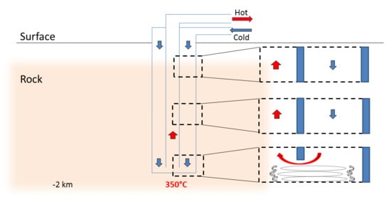
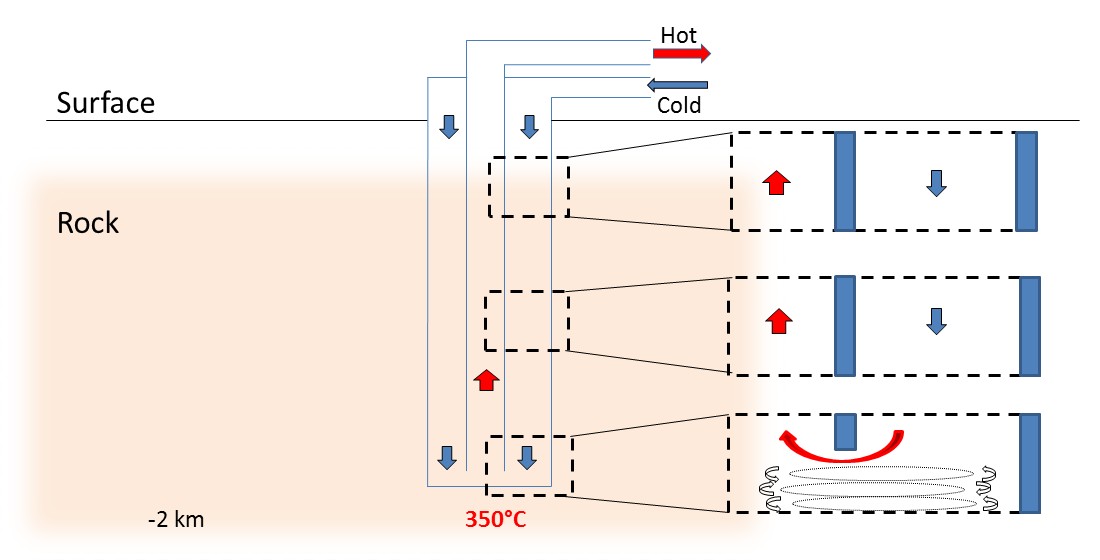
2.1. Model Parameters

The numerical study performed in this work is based on the theoretical model described in [18]. T2Well [29] uses a dedicated multiphase transient calculation coupled with the geothermal simulator TOUGH2 [32]. The calibrated T2Well model presented in [18], based on a closed DBHE system in Hawaii [13], is extended to the depth of 1990 m with a bottomhole temperature of 350 °C. The energy flow rate calculated at 1 year in this configuration does not exceed 1.4 MW [18]. Two injections of water at 10 °C are considered, at mass flow rates 2 and 10 kg/s.

Table 1. Materials constant properties applied for the fluid and well materials. Dimension of the inner casing (C1) and external casing (C2) from [13].

Properties	Water	C1	C2
Density (kg/m3)	998.2	7850	7850
Thermal Conductivity (W/m.K)	0.6	0.06	46.1
Specific heat (J/kg.K)	4182	470	470
Viscosity (kg/m.s)	0.001003
Inner/Outer radius (m)		0.0253/0.0445	0.0797/0.0889

shows the casing properties, the values of the constant water properties used in the models, and the radial dimension of the DBHE.

The thermal conductivity of the homogenous geothermal formations is set to 1.6 W/m.K and the specific heat to 870 J/kg.K. A permeability of ${10}^{-16}$ m² and a porosity of 1% are assumed for this study. The calculated values from two vertical adjacent cells in the DBHE section from the T2Well model are extracted and applied as boundary conditions for a 10 m vertical, axisymmetric CFD model. T2Well/EOS1 calculates the values at nodes in the center or an arbitrary position in a given cell (at the boundary between the well and the surroundings for N3 in Figure 2) Constant water properties and the IAPWS-IF97-based formulations for density, thermal conductivity and viscosity are separately applied in the CFD model. However, the specific heat capacity remains constant as it can only be function of temperature [30]. A time period of 1 year is considered, and data are extracted at depths of −500 m, −1900 m, and −1987 m.

Figure 2 describes the boundary conditions obtained from T2Well and applied to three CFD models, corresponding to the depth of −500 m, −1900 m, and the bottom of the DBHE. The node located at a depth of −495 m (N1-495) provides the temperature and pressure in the annular section to be applied at the outlet of the CFD model. Similarly, the N1-505 node provides the values for the inlet of the CFD model. A constant temperature boundary is applied at the face of the internal (C1) and external (C2) casing (top and bottom), equal to the values from the nodes N2 and N4. A gradient of temperature is applied onto the side wall of the well (established from the temperature values of the nodes N5-495 and N5-505), corresponding to the contact between the cement and the external casing (C2). The same strategy is considered for nodes located at the depth of −1900 m. At −1978 m, two geothermal gradients (Grad1T −1987/−1989 and Grad2T −1989/−1990) are considered to account for the large increase of temperature in the bottomhole section. A pressure inlet and a constant temperature are applied at the bottom of the internal well and top of the annular tubing, while a pressure outlet condition is applied at the top of the internal well and bottom of the annular tubing, detailed in

Table 2. Temperature (°C) and Gauge Pressure (Pa) applied in the CFD models, extracted after 1 year of simulation from the T2Well model [18]. For the node N5 of the model CFD 1987, the values stand for the temperature at depths −1978 m/−1987 m/−1989 m/−1990 m, respectively.

CFD Models	Mass Flow Rate (kg/s)	N1	N2	N3	N4	N5
		495 m/505 m
		1895 m/1905 m
		1978 m/1990 m
CFD 500	2	90.29/90.35	49.33/49.5	11.91/11.98	18.45/18.725	21.85/22.18
		4,799,675/4,896,675		4,868,875/4,967,075
	10	32.21/32.20	20.36/20.38	11.41/11.46	11.45/11.50	15.15/15.28
		7,382,175/7,530,275		23,168,675/23,266,675
CFD 1900	2	96.03/96.04	92.39/92.80	89.65/90.36	89.76/90.47	100.87/101.63
		18,393,675/28,217,675		18,488,675/18,583,675
	10	31.34/31.33	29.33/29.43	27.82/28	27.96/28.14	41.85/42.10
		28,143,675/28,291,675		36,921,675/37,019,675
CFD 1987	2	96.11/337.71	95.69/337.71	29.28/337.71	95.49/337.71	107.01/108.10
		19,195,973				108.35/337.71
	10	31.27/336.51	30.15/336.51	29.28/336.51	29.43/336.51	43.93/44.73
		2,9368,858				44.91/336.51

.

2.2. Mathematical Model of T2well

T2Well is a coupled wellbore-reservoir simulator, solving a 1D two-phase momentum equation for the wellbore and the 3D multiphase Darcy Law in the reservoir [29]. The IAPWS-IF97 formulation [31] is considered for the equation of state of water. The well and the rock formation connection are closed in order to mimic heat transfer only between the DBHE and the surroundings, without fluid flow. Kinetic energy is considered in the wellbore, where water velocity is high, but it is neglected in the porous reservoir, where low fluid velocities are present. The conservation of mass (k = 1) and energy (k = 2) for a single phase system can be written as

$$\frac{d}{dt}{{\displaystyle \int }}_{V_n}^{}{M}^{k}d{V}_n={{\displaystyle \int }}_{{\Gamma }_n}^{}{F}^k·nd{\Gamma }_n+{{\displaystyle \int }}_{V_n}^{}{q}^{k}d{V}_n$$

(1)

where V is the volume (m³), n is the outward normal vector, $\Gamma$ is the surface area of the well (m²) and q is the source or sink terms for the mass or energy component. $M^1$ is the mass accumulation term and $F^1$ is the mass flux, which are defined as

$$M^1=\rho ;F^1=\rho u$$

(2)

where ρ is the density (kg/m³), and u is the fluid velocity (m/s). In the wellbore, the energy flux accumulation is

$$F^2=-\lambda \frac{dT}{dz}-\frac{1}{A}\frac{d}{dz}\left\{A\rho (h+\frac{u^2}{2}+gzcos\theta )\right\}$$

(3)

The term A is the cross sectional area of the wellbore, θ is the angle between the vertical direction z and the wellbore section, and z is the elevation in the well.

$$M^2=\rho (U+\frac{u^2}{2}+gzcos \theta )$$

(4)

where U is the internal energy of water liquid. The momentum equation in the wellbore is

$$\frac{d}{dt}\left(\rho u\right)+\frac{1}{A}\frac{d}{dz}\left(A\rho u^2\right)=\frac{-dp}{dz}-\frac{\Omega f\rho u^2}{2A}-\rho gcos\theta$$

(5)

with $\Omega$ the perimeter of the cross section, $f$ the apparent friction defined as $f$ = 16/Re when Re < 2400, and as follows when Re > 2400:

$$\frac{1}{\sqrt{f}}= -4log\left[\frac{\frac{2\delta }{d}}{3.7}-\frac{5.02}{Re}log\left(\frac{\frac{2\delta }{d}}{3.7}+\frac{13}{Re}\right)\right]$$

(6)

where $\delta$ is the roughness of the well walls and Re is the Reynolds number, defined as Re = $\rho ud/\mu$ with d the diameter of the well or, corrected for an annulus via the hydraulic diameter (d_o − d_i), and μ the water viscosity. The formulations for the energy flux, accumulation and fluid velocity in the porous reservoir can be found in [29]. The artificial increase of the annulus perimeter, as mentioned in [19], is used to calibrate the T2Well DBHE model from the experimental pressure data from [13]. More details on the T2Well mathematical model used for the DBHE model are provided in [18].

2.3. Mathematical CFD Model

The governing equations are solved with the CFD code ANSYS Fluent 17.1.0, which is based on the finite volume method [30]. The k − ε realizable turbulence model is applied in the simulations. For an axisymmetric model, the continuity equation is written as

$$\frac{\partial \rho }{\partial t}+\frac{\partial \left(\rho u_z\right)}{\partial z}+\frac{\partial \left(\rho u_r\right)}{\partial r}+\frac{\rho u_r}{\partial r}=0$$

(7)

The momentum equations are defined by the following equations:

$$\begin{array}{ccc}\hfill \frac{\partial \left(\rho u_z\right)}{\partial t}& +& \frac{1}{r}\frac{\partial \left(r\rho u_z{u}_z\right)}{\partial z}+\frac{1}{r}\frac{\partial \left(r\rho u_r{u}_z\right)}{\partial r}\hfill \\ & & =-\frac{\partial \rho }{\partial z}+\frac{1}{r}\frac{\partial \left[r\mu \left(2\frac{\partial u_z}{\partial z}\right)-\frac{2}{3}\left(\nabla ·\overrightarrow{u}\right)\right]}{\partial z}+\frac{1}{r}\frac{\partial \left[r\mu \frac{\partial u_z}{\partial r}-\frac{\partial u_r}{\partial z}\right]}{\partial r}+ \rho \overrightarrow{g}\hfill \end{array}$$

(8)

$$\begin{array}{ccc}\hfill \frac{\partial \left(\rho u_r\right)}{\partial t}& +& \frac{1}{r}\frac{\partial \left(r\rho u_z{u}_r\right)}{\partial z}+\frac{1}{r}\frac{\partial \left(r\rho u_r{u}_r\right)}{\partial r}\hfill \\ & & =-\frac{\partial \rho }{\partial r}+\frac{1}{r}\frac{\partial \left[r\mu \left(\frac{\partial u_r}{\partial z}+\frac{\partial u_z}{\partial r}\right)\right]}{\partial z}+\frac{\partial \left[r\mu \left(2\frac{\partial u_r}{\partial r}\right)-\frac{2}{3}\left(\nabla ·\overrightarrow{u}\right)\right]}{\partial r}-2\mu \frac{u_r}{r^2}\hfill \\ & & +\frac{2\mu }{3r}\left(\nabla ·\overrightarrow{u}\right)\hfill \end{array}$$

(9)

where u is the fluid velocity and μ its molecular viscosity. The energy equations in the fluid and solid zone are

$$\frac{\partial \left(\rho E\right)}{\partial t}+(\nabla ·(\overrightarrow{u(}\rho E+p))=\nabla ·(k_{eff}\nabla T- {\displaystyle \sum }h\overrightarrow{J}+(\stackrel{=}{{\tau }_{eff}}·\overrightarrow{u}))$$

(10)

$$\frac{\partial \left(\rho h\right)}{\partial t}-\lambda \nabla T=0$$

(11)

${\lambda }_{eff}$ is the effective thermal conductivity $\lambda +{\lambda }_t$, with ${\lambda }_t$ the turbulence thermal conductivity. ${\lambda }_t$ is described by c${\mu }_t/0.85$, with c and ${\mu }_t$ the specific heat capacity and the turbulent viscosity, respectively. The stress tensor ${\tau }_{eff}$ is defined and can be retrieved from [30]. The energy E and the sensible enthalpy h are calculated via Equation (12):

$$E = {{\displaystyle \int }}_T^{Tref}c dT+ \frac{p}{\rho }+ \frac{u^2}{2}$$

(12)

The standard turbulence k − ε model is based on transport equations for the turbulence kinetic energy (k) and its dissipation rate (ε) [30]. This model is fast and has proved to be efficient at high speed and suitable for numerous industrial applications. Continuum equations can be written as

$$\frac{\partial \left(\rho k\right)}{\partial t}+\frac{\partial \left(\rho k{u}_z\right)}{\partial z}=\frac{\partial }{\partial r}\left(\left(\mu +{\mu }_t\right)\frac{\partial k}{\partial r}\right)+G_k+G_b-\rho \epsilon -Y_M$$

(13)

$$\frac{\partial \left(\rho \epsilon \right)}{\partial t}+\frac{\partial \left(\rho \epsilon u_z\right)}{\partial z}=\frac{\partial }{\partial r}\left(\left(\mu +\frac{{\mu }_t}{1.2}\right)\frac{\partial \epsilon }{\partial r}\right)+\rho C_{1}S-\rho C_2\frac{{\epsilon }^2}{k+\sqrt{u\epsilon }}+C_{1\epsilon }\frac{\epsilon }{k}{C}_{3\epsilon }{G}_b$$

(14)

with the eddy viscosity ${\mu }_t$, S, $C_1,C_{3\epsilon }$ described in [30]. $C_{1\epsilon }$ and $C_2$ are respectively equal to 1.44 and 1.99 by default. The different terms present in the continuum equation for both T2Well and Fluent are reported in

Table 3. Terms in continuum equation.

${\mathit{G}}_{\mathit{k}}$	${\mathit{G}}_{\mathit{b}}$	${\mathit{Y}}_{\mathit{M}}$
$-\rho \overline{u_z{u}_r}\frac{\partial u_r}{\partial z}$	$-\frac{g_z}{\rho }{\left(\frac{\partial \rho }{\partial T}\right)}_P\frac{{\mu }_t}{0.85\rho }\frac{\partial \rho }{\partial z}$	$2\rho \mathsf{\epsilon }\frac{k}{\propto RT}$

.

$G_k$ and $G_b$ are the generation of turbulence kinetic energy, accounting for the mean velocity gradient, and due to buoyancy when the water properties are not constant, respectively. $Y_M$ represents the contribution of the fluctuating dilatation in compressible turbulence to the overall dissipation rate [30], $\propto$ is the speed of sound in the fluid.

The turbulent heat transport uses the Reynold’s momentum transfer such as

$$\frac{\partial \left(\rho E\right)}{\partial t}+\frac{\partial \left(u_z\left(\rho E+p\right)\right)}{\partial z}=\frac{\partial }{\partial r}\left({\lambda }_{eff}\frac{\partial T}{\partial r}+u_z{\tau }_{eff}\right)$$

(15)

Gravity is accounted for in the numerical simulation. A convergence criterion of 10⁻⁸ was used for all equations of the flow solver, ensuring a good convergence of the flow solution. The simple scheme is selected for the pressure velocity coupling. A second order spatial discretization is used for the pressure. Turbulent kinetic, dissipation rate, energy, and momentum spatial discretization are set to the second order upwind. Table 2 summarizes the boundary conditions applied (pressure and temperature) in the CFD models. The roughness on the well walls is set to 2.5 × 10⁻⁵ m.

2.4. Mesh Independence Study

A mesh independence study is performed to make sure the results do not depend on the mesh density. The pressure inlet boundaries are artificially set to 5 bar at 209.85 °C for the internal tubing and 110 °C for the annulus. The pressure outlet is fixed at 1 bar. In this section, all boundaries are set without heat flux except for the external casing (C2) where a constant temperature value of 250 °C is applied. Three meshes of 43,500, 171,656, and 514,968 cells are built and used in a steady-state solver. Figure 3a shows the radial temperature distribution in the middle of the model, which highlights a high degree of convergence between all three meshes. Figure 3b uses a narrower range of temperature which shows the incremental increase of temperature as the distance from the axis of the well increases. As expected, the trend is smoother when using more cells, but it shows that the intermediate and fine grid results are very close.

Based on the computational cost of a simulation, the intermediate mesh (171,656 cells) has been selected. This mesh ensures a smooth increase of the temperature, preventing divergence problems, which is a problem easily faced when using the IAPWS-IF97 formulation [31], which was applied through a user defined function (UDF) called at each time step of the simulation.

A similar methodology has been applied to the third CFD model at the bottom of the DBHE (CFD 1987). This model contains 809,676 cells.

3. Results

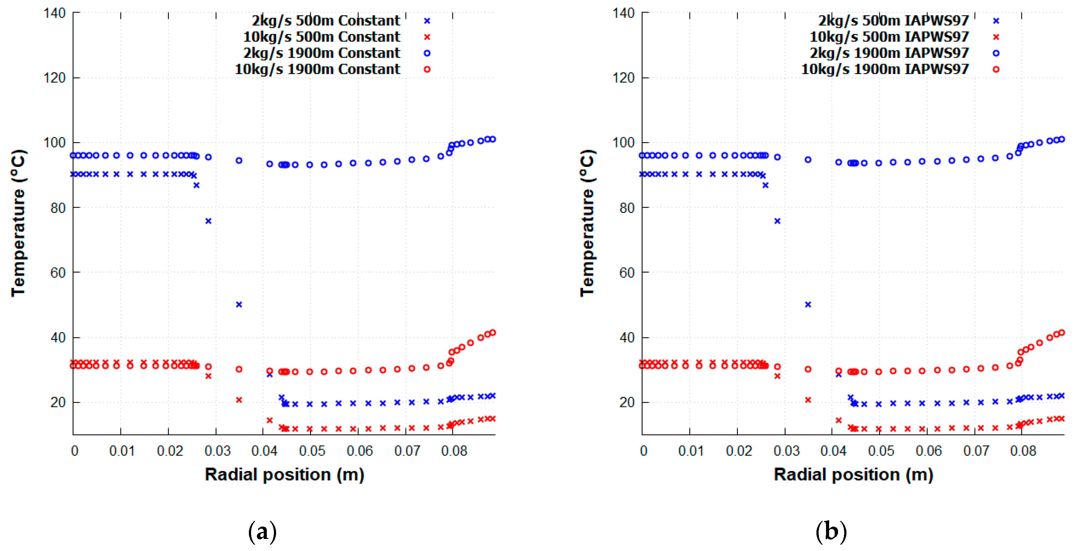
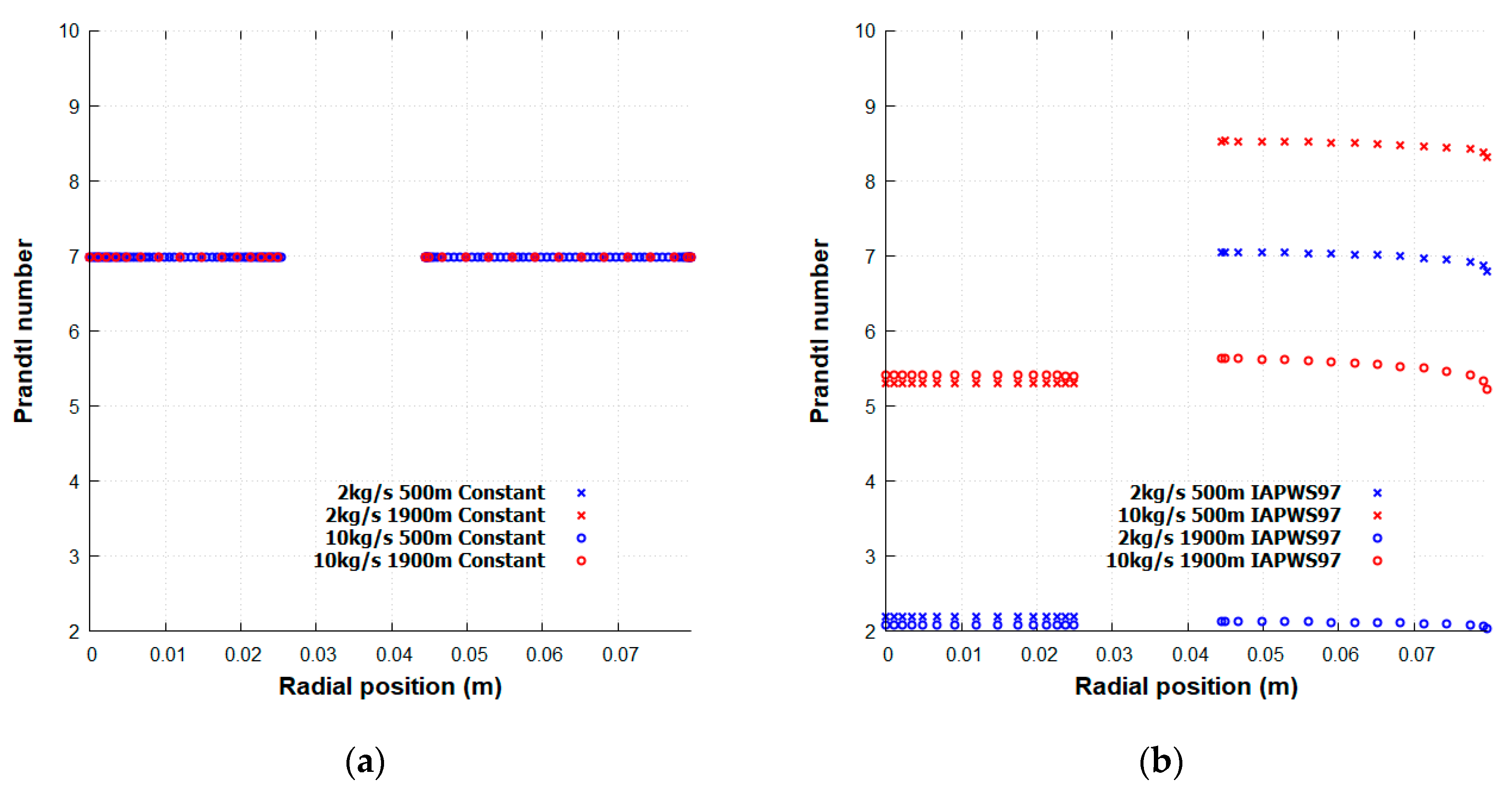
3.1. Vertical Comparison Analysis at −500 m and −1900 m

3.1.1. Thermal Analysis

In the two CFD models corresponding to the depths of −500 m and −1900 m (CFD 500 and CFD 1900), the pressure inlet and outlet conditions are linked to an imposed mass flow rate. Thus, the pressure field is accurately constrained in the production and injection wells compared to the T2Well values.

Figure 4 shows the vertical temperature in the center of production well (inner tubing) and in the injection well (annular, taken at a 6 cm radial distance from the axis) after 1 year. In the production well, the CFD-based temperatures at −495 m are comparable (less than 1 °C difference) to the values obtained with T2Well. However, in the annulus section, the calculated steady state temperature shows increased values in the range of 1.3 °C and 8.0 °C.

In all cases except when having a mass flow rate of 2 kg/s at 500 m (Figure 4f), no temperature difference could be noticed between results based on the IAPWS-IF97 formulation and those obtained with constant water properties. In Figure 4f, however, the use of constant water properties seems to underestimate the temperature distribution by 1 °C. The very low increase of temperature between the bottom and top of the production well (upwarding fluid) in Figure 4c,e,g is in agreement with the T2Well trend.

While the inlet injections in all wells (bottom for the production well and top for the injection well) match the T2Well values, the outlet velocities are higher, with a maximum amplitude of 0.2 m/s for a mass flow rate of 2 kg/s, and 0.85 m/s for 10 kg/s, respectively.

3.1.2. Fluid Properties Analysis

Table 4. Error between the constant values and the IAPWS-IF97 in the vertical axis for the density, thermal conductivity and viscosity (in %). The left side of each cell (3.1/) is for the production well and right side (/ −0.22) is for the annulus. The negative values are set for lower values using the IAPWS-IF97 properties compared to the constant values.

Depth	Density		Thermal	Conductivity	Viscosity
	2 kg/s	10 kg/s	2 kg/s	10 kg/s	2 kg/s	10 kg/s
500 m	3.10/−0.22	0/0.2	−12.62/−0.26	−3.66/0.30	68.66/−0.52	24.11/−21.71
1900 m	2.87/2.74	−0.91/−1.33	−14.32/−14.17	−5.23/−5.59	70.22/69.61	22.63/20.11

shows the error between the results obtained when using constant density, thermal conductivity, and viscosity values and those obtained when using the IAPWS-IF97-based formulations. Results based on a constant density show an error less than 5% compared to those obtained with pressure temperature dependent densities. For the water thermal conductivity, the error increases with a low mass flow rate at a greater depth (up to 14% overestimated). Pressure and temperature values are higher, showing that the assumption of constant surface water properties should not be considered. The viscosity shows the highest differences, up to 70% overestimation in the production well.

3.2. Radial Comparison Analysis at −500 m and −1900 m

3.2.1. Thermal Analysis

Figure 5 shows the radial temperature distribution obtained with the CFD models at the depth of 500 m and 1900 m for a mass flow rate injection of 2 kg/s and 10 kg/s with constant (a) and the IAPWS-IF97 water properties (b), respectively. The radial temperatures in the well are homogeneous in the production well (0–0.0253 m), which can validate the use of the 1D area average calculation in T2Well, for this part. However, the injection well shows a small increase of temperature (up to 5 °C) next to Casing 2. As T2Well computes the injection well temperature very close to Casing 2 for a given elevation (z or x) at the radial position of 0.0797 m, an over-estimation of the temperature in the injection well by 2–4 °C is expected when applying a 1D approach.

3.2.2. Heat Transfer Analysis

The production well extracts the energy, with a surface heat flux on the casing wall higher than 100 W/m². The radial Prandtl number in water at the depth of −500 m (a) and −1900 m (b) are presented in Figure 6. As the water specific heat is constant in this study, the Prandtl number reveals only the ratio of the viscosity and the thermal conductivity. This allows to identify the predominance of heat transfer convection (Pr >> 1) or conduction (Pr << 1). Figure 6 shows that Pr is higher than 1, with the lowest values obtained for a mass flow rate of 2 kg/s in Figure 6b. When constant thermal conductivity and viscosity values are applied, the Pr reaches 6.9.

Using the IAPWS IF97 properties, a higher mass flow rate shows a high Pr number. The convective heat transfer is higher due to the high water velocity and larger temperature difference between the fluid and its surroundings. In the annulus at 500 m for both mass flow rates, the Pr number rises due to the high temperature drop between the annulus and the tubing shown in Figure 5.

Except for the 10 kg/s at 500 m case, the use of constant values in this study tends to overestimate the convective heat transfer. The Prandtl number shows a low decrease at the wall boundary in the injection well, outlining a higher conductive heat transfer effect in the vicinity of the well wall.

3.3. Return Flow Analysis

3.3.1. Pressure and Temperature Comparison

At the bottom of the DBHE, water returns to the surface from the annular well to the producing well. In this study, 3 m separate the bottom of the internal tubing from the bottom of the DBHE. Figure 7 shows the static pressure distribution in the bottom of the well for a mass flow rate injection of 2 kg/s (a) and 10 kg/s (b) with constant water properties, and with the IAPWS-IF97 properties (c,d).

Table 5. Pressure and temperature in DBHE at −1987 m based on the CFD and T2Well results.

	Pressure in the Annular at −1987 m (Pa/bar)		Temperature in the Internal tubing at −1987 m (K)
	2 kg/s	10 kg/s	2 kg/s	10 kg/s
CFD constant	1.92281 × 107/192	2.97761 × 107/297	375.08	305.39
CFD IAPWS-IF97	1.92272 × 107/192	2.97752 × 107/297	375.43	302.43
T2Well	1.92748 × 107/192	3.77324 × 107/377	369.26	304.42

summarizes the results of pressure in the annular and temperature in the internal tubing at −1987 m obtained with the CFD model and with T2well. For the CFD-based results, using the IAPWS-IF97 properties implies a small decrease in the pressure distribution (<1000 bars) and similar temperature results with a mass flow rate of 2 kg/s.

Increasing the mass flow rate with the IAPWS-IF97 properties shows a decrease of the water temperature in the internal tubing at −1987 m when compared to constant properties based results.

The pressure calculated with ANSYS Fluent is similar to the T2Well results in the case of 2 kg/s and higher by three bars at 10 kg/s. At low mass flow rate, the CFD temperatures are higher by 5 °C and in similar range at 10 kg/s. The pressure correction applied in T2Well, calibrated with the experimental data in [18], deviates at high mass flow rate, with an overestimation of 80 bars. Thus, the estimation of the circulating water power consumption in the DBHE from the CFD study, suggests a lower value than reported by the authors in [19].

With a mass flow rate of 2 kg/s, the static pressure in the fluid is lower than for 10 kg/s. The pressure decreases in the internal tubing compared to the annular well, with a local depression near the bottom of the internal tubing. This pressure difference is higher when considering a mass flow rate of 10 kg/s. Thus, the fluid is accelerated in this section of the DBHE (see Section 3.3.2).

Furthermore, the constant boundary conditions applied on the side of the CFD model might be slightly overestimated compared to the T2Well values. As the distance of the node N5 (see Figure 2) to the casing wall is not negligible, the temperature obtained with T2Well is potentially slightly higher than considered in the casing wall with the CFD model.

3.3.2. Velocity Field Analysis

Figure 8 presents the velocity distribution for the mass flow rate injection at the bottom of the DBHE. In agreement with the pressure decreases shown in Figure 7, water accelerates at the bottom of the internal tubing.

A lower fluid velocity is noticed for a low mass flow rate injection. When water returns to the surface, a very low velocity zone (5 cm) is observed on the external side of the internal tubing. The use of the IAPWS-IF97 properties for water leads to higher velocity values at 2 kg/s and slightly lower velocities at 10 kg/s.

Figure 9 shows the turbulence kinetic energy at the bottom of the DBHE. The turbulence kinetic energy appears mainly localized in the low velocity zone (visible in Figure 8) and at the center of the annular well, where water accelerates. As expected, the turbulence kinetic energy is also higher when the injection mass flow rate is higher. For 2 kg/s and 10 kg/s, approximate pressure differences of 1 and 4 bar are obtained, respectively, between the pressure in the annular and the internal tubing. Due to higher velocities values at high mass flow rates, frictions are generated in the bottom of the well, increasing the pressure drop.

3.3.3. Convection Analysis

Figure 10 shows the convective cells in the bottom of the DBHE, below the internal tubing when the IAPWS-IF97 properties are used in the CFD model. The velocity vectors are presented in Figure 10a and the axial component of the velocity in Figure 10b in the vertical axis and at the radial distance of 6 cm (i.e., in the middle of the production well). For both injection mass flow rates, three convective cells are observed, with similar intensity. At the bottom of the DBHE (last 1 m), water rises near the well and flows down in the center. The water velocities are lower than 0.2 m/s. A second convective cell is observed with lower velocity values connected to a small cell next to the internal tubing depth. Using constant or IAPWS-IF97-based properties for modeling water circulation opens the discussion for a deeper analysis and a more thorough description of the thermodynamics in the current heat transfer calculation at the bottom of a DBHE when using a 1D code.

4. Discussion

Despite not having considered the specific heat of water as a pressure–temperature dependent property in ANSYS Fluent, the heat transfer calculation between the CFD model and T2Well is similar, with a more detailed description of the physics when considering the CFD approach. After a simulated time period of 1 year using the IAPWS-IF97, the maximum density difference against the average value in the radial axis is less than 2% and less than 9% for the viscosity, mainly in the injection well. For the radial axis, the velocity variation reaches up to 5% in the production well and 20% in the injection well. The stagnant boundary of the water at the wall (v = 0) shows a local conductive heat transfer, impacting the convective heat transfer when the roughness of the well is high with high velocity (lower mean temperature in the well than at the contact of the well wall in Figure 4). Thus, the 1D calculation shows a slight increase of the mean temperature in a cross section of the DBHE. However, the constant geothermal gradient value used in the CFD models is subject to discussion due to the distance to the wall, mentioned in Section 3.3.1.

In the formal analysis of the energy equation, the thermal conductivity in T2well is an area averaged value considering the fluid and the casing material. As the casing thermal conductivity is higher than water, the area averaged value calculated can be higher than the water value only. This might tend to slightly overestimate the heat transfer using T2Well.

Further development can be achieved in the CFD model to deliver a pressure dependent formulation for the specific heat of pure water.

The return pressure estimated with T2Well appears highly overestimated at high mass flow rates. Despite being calibrated with an experimental study, the artificial pressure constrains used in T2Well need to be equilibrated for high mass flow rates, to avoid the overestimation of the energy and power consumed to transport water in DBHEs in high geothermal gradients. By evaluating lower pressure losses in the return flow, the CFD modelling tends to lower the pressure drop between the annular and tubing flow compared to the 1D approach. Thus, the energy consumption to impose a high pressure in the annulus of a DBHE might be subject to a re-evaluation using detail numerical models, or experimental data, if available.

The existence of independent convective cells at the bottom of the internal tubing opens new perspectives to optimize their intensity, notably with high conductive materials on the wellbore [27], to stimulate self-convection following the energy demand. Using both 1D and 2D-axisymmetric approaches enable to strengthen the heat transfer and fluid flow estimation from unconventional geothermal well designs. Due to the computational costs associated with CFD, it is advised to apply such techniques after a large set of 1D simulations is complete, or when a more detailed analysis is required.

5. Conclusions

This double numerical approach has aimed to refine the fluid flow and heat transfer numerical calculation in a DBHE in high geothermal gradient. A conjugated numerical use of T2Well-1D well formulation with three 2D axisymmetric CFD models from a theoretical DBHE set at 1900 m in volcanic formations with 350 °C at the depth of 2000 m, has been performed. A CFD approach refines the 1D description, considering the vertical and radial velocity distribution along with turbulence and local wall boundary effects. The difference of results highlighted in this work allows to discuss both approaches. Local wall boundary effects due to the well roughness decrease the mean temperature in the production well. The use of ANSYS Fluent and T2Well opens new perspectives to investigate and engineer DBHEs with pure liquid water. To estimate the energy produced from DBHEs, the use of constant water properties in the CFD model underestimates the overall heat transfer at high temperatures (more than 80 °C) at low mass flow rate (2 kg/s). It is advised to consider pressure–temperature dependent formulations for the water properties, to reduce uncertainties in the numerical modelling of a DBHE in high geothermal gradient areas.

Self-convective water cells are observed at the bottom of the DBHE, with no significant changes with water flow rate. The pressure losses associated with the return flow at the bottom of the DBHE are refined with CFD compared to a 1D approach, corresponding to a large pressure difference of 80 bars at a flow rate of 10 kg/s. Previous evaluations of the energy extracted and consumed in a DBHE can be discussed with lower expected return pressures. The conjugated numerical approach significantly improves the understanding of fluid flow and heat transfer in DBHEs in high geothermal gradients environments, which will allow further technological advances.

References

1. Davies, J.H.; Davies, D.R. Earth’s surface heat flux. Solid Earth Discuss. 2009, 1, 1–45. [Google Scholar] [CrossRef]
2. Bertani, R. Geothermal power generation in the world 2005–2010 update report. Geothermics 2012, 41, 1–29. [Google Scholar] [CrossRef]
3. Tester, J.; Morris, G.; Cummings, R.; Bivins, R. Electricity from Hot Dry Rock geothermal Energy: Technical and Economic Issues; Los Alamos Scientific, Laboratory: Los Alamos, NM, USA, 1979. [Google Scholar]
4. Alimonti, C.; Conti, P.; Soldo, E. A comprehensive exergy evaluation of a deep borehole heat exchanger coupled with a ORC plant: The case study of Campi Flegrei. Energy 2019, 189, 116100. [Google Scholar] [CrossRef]
5. Falcone, G.; Liu, X.; Okech, R.R.; Seyidov, F.; Teodoriu, C. Assessment of deep geothermal energy exploitation methods: The need for novel single-well solutions. Energy 2018, 160, 54–63. [Google Scholar] [CrossRef] [Green Version]
6. Song, X.; Shi, Y.; Li, G.; Shen, Z.; Hu, X.; Lyu, Z.; Zheng, R.; Wang, G. Numerical analysis of the heat production performance of a closed loop geothermal system. Renew. Energy 2018, 120, 365–378. [Google Scholar] [CrossRef]
7. Westaway, R. Deep Geothermal Single Well heat production: Critical appraisal under UK conditions. Q. J. Eng. Geol. Hydrogeol. 2018, 51, 424–449. [Google Scholar] [CrossRef]
8. Alimonti, C.; Soldo, E.; Bocchetti, D.; Berardi, D. The wellbore heat exchangers: A technical review. Renew. Energy 2018, 123, 353–381. [Google Scholar] [CrossRef]
9. Oldenburg, C.M.; Pan, L.; Muir, M.P.; Eastman, A.D.; Higgins, B.S. Numerical simulation of critical factors controlling heat extraction from geothermal systems using a closed-loop heat exchange method. In Proceedings of the 41st Workshop on the Geothermal Reservoir Engineering, Stanford University, Stanford, CA, USA, 22–24 February 2016. [Google Scholar]
10. Templeton, J.; Ghoreishi-Madiseh, S.; Hassani, F.P.; Al-Khawaja, M. Abandoned petroleum wells as sustainable sources of geothermal energy. Energy 2014, 70, 366–373. [Google Scholar] [CrossRef]
11. Nian, Y.-L.; Cheng, W.-L.; Yang, X.-Y.; Xie, K. Simulation of a novel deep ground source heat pump system using abandoned oil wells with coaxial BHE. Int. J. Heat Mass Transf. 2019, 137, 400–412. [Google Scholar] [CrossRef]
12. Watson, S.; Falcone, G.; Westaway, R. Repurposing Hydrocarbon Wells for Geothermal Use in the UK: The Onshore Fields with the Greatest Potential. Energies 2020, 13, 3541. [Google Scholar] [CrossRef]
13. Morita, K.; Bollmeier, W.S.; Mizogami, H. An Experiment to Prove the Concept of the Downhole Coaxial Heat Exchanger (DCHE) in Hawaii; Geothermal Resources Council: Davis, CA, USA, 1992. [Google Scholar]
14. Dai, C.; Li, J.; Shi, Y.; Zeng, L.; Lei, H. An experiment on heat extraction from a deep geothermal well using a downhole coaxial open loop design. Appl. Energy 2019, 252, 113447. [Google Scholar] [CrossRef]
15. Renaud, T.; Verdin, P.; Falcone, G. Numerical simulation of a Deep Borehole Heat Exchanger in the Krafla geothermal system. Int. J. Heat Mass Transf. 2019, 143, 118496. [Google Scholar] [CrossRef]
16. Bu, X.; Ma, W.; Li, H. Geothermal energy production utilizing abandoned oil and gas wells. Renew. Energy 2012, 41, 80–85. [Google Scholar] [CrossRef]
17. Le Lous, M.; Larroque, F.; Dupuy, A.; Moignard, A. Thermal performance of a deep borehole heat exchanger: Insights from a synthetic coupled heat and flow model. Geothermics 2015, 57, 157–172. [Google Scholar] [CrossRef]
18. Renaud, T. Forced Convection Heat Transfer in Unconventional Geothermal Systems Numerical Investigation of Complex Flow Processes Neat Magmatic Chambers. Ph.D. Thesis, Cranfield University, Cranfield, UK, February 2020. [Google Scholar]
19. Renaud, T.; Verdin, P.; Falcone, G.; Pan, L. Heat transfer modelling of an unconventional, closed-loop geothermal well. In Proceedings of the World Geothermal Congress, Reykjavik, Iceland, 26 April–2 May 2020. [Google Scholar]
20. Noorollahi, Y.; Pourarshad, M.; Jalilinasrabady, S.; Yousefi, H. Numerical simulation of power production from abandoned oil wells in Ahwaz oil field in southern Iran. Geothermics 2015, 55, 16–23. [Google Scholar] [CrossRef]
21. Tang, H.; Xu, B.; Hasan, A.R.; Sun, Z.; Killough, J. Modeling wellbore heat exchangers: Fully numerical to fully analytical solutions. Renew. Energy 2019, 133, 1124–1135. [Google Scholar] [CrossRef]
22. Alimonti, C.; Soldo, E. Study of geothermal power generation from a very deep oil well with a wellbore heat exchanger. Renew. Energy 2016, 86, 292–301. [Google Scholar] [CrossRef]
23. Chen, C.; Shao, H.; Naumov, D.; Kong, Y.; Tu, K.; Kolditz, O. Numerical investigation on the performance, sustainability, and efficiency of the deep borehole heat exchanger system for building heating. Geotherm. Energy 2019, 7, 18. [Google Scholar] [CrossRef] [Green Version]
24. Hu, X.; Banks, J.; Wu, L.; Liu, W.V. Numerical modeling of a coaxial borehole heat exchanger to exploit geothermal energy from abandoned petroleum wells in Hinton, Alberta. Renew. Energy 2020, 148, 1110–1123. [Google Scholar] [CrossRef]
25. Sui, D.; Wiktorski, E.; Røksland, M.; Basmoen, T.A. Review and investigations on geothermal energy extraction from abandoned petroleum wells. J. Pet. Explor. Prod. Technol. 2019, 9, 1135–1147. [Google Scholar] [CrossRef]
26. Heller, K.; Teodoriu, C.; Falcone, G. A new deep geothermal concept based on the geyser principle. In Proceedings of the 39th Workshop Geothermal Reservoir Engineering, Stanford University, Stanford, CA, USA, 24–26 February 2014. [Google Scholar]
27. Hara, H. Geothermal Well Using Graphite as Solid Conductor. U.S. Patent Application US20110232858A1, 29 September 2011. [Google Scholar]
28. Cheng, W.-L.; Li, T.-T.; Nian, Y.-L.; Xie, K. Evaluation of working fluids for geothermal power generation from abandoned oil wells. Appl. Energy 2014, 118, 238–245. [Google Scholar] [CrossRef]
29. Pan, L.; Oldenburg, C.M. T2Well—An integrated wellbore–reservoir simulator. Comput. Geosci. 2014, 65, 46–55. [Google Scholar] [CrossRef]
30. ANSYS. Ansys Fluent Theory Guide; Volume Release 17; ANSYS: Canonsburg, PA, USA, 2016. [Google Scholar]
31. Wagner, W.; Cooper, J.R.; Dittmann, A.; Kijima, J.; Kretzschmar, H.-J.; Kruse, A.; Mares, R.; Oguchi, K.; Sato, H.; Sto¨cker, I.; et al. The IAPWS Industrial Formulation 1997 for the Thermodynamic Properties of Water and Steam. J. Eng. Gas Turbines Power 2000, 122, 150–184. [Google Scholar] [CrossRef]
32. Pruess, K.; Oldenburg, C.; Moridis, G. TOUGH2 User’s Guide. Earth Sciences Division; Lawrence Berkeley National Laboratory, University of California: Berkeley, CA, USA, 2012.
Figure 1. Schematic of the downhole borehole heat exchanger concept set in Hawaii above a magmatic intrusion (modified from [13]).
Energies 13 06107 g001
Figure 2. Schematic of the T2Well model [18] used to extract the boundary conditions applied in the 3 computational fluid dynamics techniques (CFD) models at the depth of 500 m (CFD 500), 1900 m (CFD 1900) and at the last 12 m of the deep geothermal heat exchangers (DBHE) (CFD 1987).
Energies 13 06107 g002
Figure 3. Mesh-independence study for the CFD model—(a) Radial Temperature taken in the middle of the model (at 5 m); (b) Focus on the radial temperature in the internal tubing.
Energies 13 06107 g003
Figure 4. Temperature distribution in the production (a,c,e,g) and injection well (b,d,f,h) at the depth of 500 m (ad), 1900 m (eh) for the mass flow rate of 2 kg/s (a,b,e,f), 10 kg/s (c,d,g,h) compared to the T2Well temperature values taken after a simulating period of 1 year.
Energies 13 06107 g004
Figure 5. CFD study. (a) CFD-based radial Temperature distribution at −500 m and −1900 m with constant water properties. (b) CFD-based radial Temperature distribution at −500 m and −1900 m using the IAPWS IF97 properties. The blue values are set for the mass flow rate injection of 2 kg/s and the red values for 10 kg/s.
Energies 13 06107 g005
Figure 6. CFD study. (a) Radial Prandtl number at −500 m and −1900 m for constant water properties. (b). Radial Prandtl number at −500 m and −1900 m using the IAPWS IF97 properties.
Energies 13 06107 g006
Figure 7. CFD study. Static pressure distribution at the bottom of the internal tubing for a mass flow rate injection with constant water properties of 2 kg/s (a) and 10 kg/s (b) and with the IAPWS-IF97 properties for 2 kg/s (c) and 10 kg/s (d).
Energies 13 06107 g007
Figure 8. Velocity distribution at the bottom of the internal tubing for a mass flow rate injection with constant water properties of 2 kg/s (a) and 10 kg/s (b) and with the IAPWS-IF97 properties for 2 kg/s (c) and 10 kg/s (d).
Energies 13 06107 g008
Figure 9. Turbulence Kinetic Energy distribution at the bottom of the internal tubing for a mass flow rate injection with constant water properties of 2 kg/s (a) and 10 kg/s (b) and with the IAPWS-IF97 properties for 2 kg/s (c) and 10 kg/s (d).
Energies 13 06107 g009
Figure 10. CFD results. (a) Velocity vectors at 2 kg/s using the IAPWS-IF97 properties below the internal tubing with the interpretation of the convective cells. The vertical axis has been scaled 40 times compared to the radial axis in order to visualize 3 m. (b) Axial velocity in the vertical axis (Production axis) and Injection axis (r = 0.06 m). The negative values indicate ascending water. The positive values stand for the descending water.
Energies 13 06107 g010