Abstract
Power lines are often placed in ground or sea water, which are weakly conductive media. In the paper, a new analytical formula, taking into account the proximity effect in a twin line placed in a weakly conductive medium, is derived, and the effect of the conductive medium is considered. In the first step, one of the wires is replaced by a current filament, and the solution is sought for magnetic vector potential around the filament. In the next step, an analytical formula for eddy currents induced in a long straight conductor of circular cross-section placed near to the current filament in the extensive conductive medium is found by using the method of separation of variables. The correctness of the formula is checked by comparison with the results obtained via other methods like finite and boundary element methods. Then, the effect of various parameters on the eddy current distribution is tested. Next, the proximity effect in a twin symmetrical line is considered, and the effect of the conductivity of the surrounding medium is investigated. The results indicate that the conductive medium weakens the proximity effect, but in typical cases (ground and sea water), the effect is very small.
1. Introduction
Round wires are often used in power and signal transmission. The higher the electrical conductivity, magnetic permeability, cross-section radius, and frequency of currents in a wire, the less current passes through the central layers of the wire and more current passes in the superficial layers. This phenomenon is known as the skin effect and is a result of electromagnetic induction. If two or more conductors are placed in the vicinity, electromagnetic induction generates eddy currents in the neighboring wires, and the current density becomes additionally disturbed. This is known as the proximity effect. The two effects impact greatly the current distribution inside the wires and, consequently, the impedance of a system, which reflects then in increased voltage drops and increased losses in such lines. Therefore, the knowledge of current density distribution in the conductors is very important in the calculations of network properties of such lines. Starting from Maxwell [1], a lot of research has been performed so far in this field, and many analytical and numerical methods have been developed. One of the first approaches was presented by Manneback [2], who developed an integral equation for skin effect in parallel conductors. Dwight [3] considered the proximity effect in thin tubes. The approach was later expanded in [4,5] and used to model power and signal lines with neighboring wires substituted with current filaments [6,7,8]. A similar method was later presented in works [9,10]. Jabłoński [11] considered a general solution for round wire affected by an arbitrary time-harmonic magnetic field. At the same time, various numerical methods were used in this field. Rolicz proposed Galerkin + variable separation method [12]. Jabłoński used boundary elements with specific approximation [13]. Piątek et al. used a numerical approach based on the integral equation [14]. A similar method was proposed by Coufal [15] or Freitas et al. [16]. Besides, the finite elements were often involved [17,18,19]. Pagnetti et al. [20], and independently Jabłoński et al. [21], proposed a numerical-analytical method, generalizing the approach with substitutive current filaments.
All of the above-mentioned works considered wires placed in a non-conductive medium. However, power and transmission lines are sometimes placed in the ground or in the sea [22], which are conductive media, although of electrical conductivity much less than that of typical metals used for electrical wires, e.g., copper. It is worth investigating two commonly encountered conductive media: ground and water. The conductivity of ground (soil or rock) is highly dependent on moisture and composition. For low frequencies, the typical values of electrical conductivity for soils and rocks are from 0.01–1 mS/m for loose sands to 1 S/m for some clays [23]. The electrical conductivity of water depends on the content of cations and anions. Typical values are from around 1–3 mS/m for rainwater [24] to around 5–6 S/m for sea water [25]. Since the problem for more than one wire of finite cross-section has no exact closed solution (excluding the cables of cylindrical symmetry), there are two ways to deal with the problem: using numerical methods or using approximate analytical formulas. Both approaches are approximate, and both have pros and cons. Numerical methods allow us to take into account realistic aspects, but obtaining general conclusions is difficult. In contrast, analytical methods require usually more simplifications but offer formulas, which can be very useful within certain limits. One of the earliest analytical approaches was proposed by Pollaczek [26], who found a formula for electric field induced due to current filament buried in the ground at a certain depth. Several other more or less similar analytical approaches can also be found in the literature. Machado and da Silva developed an analytical approach for underground cables via power series expansion [27,28]. This solution requires calculating rather complicated integrals. A generalization of this approach was described by Tsiamitros et al. [29]. At the same time, numerical methods, especially finite elements, were used [30,31]. The magnetic field of underground cables was considered in works [32,33]. Later, Brito et al. used their previous results for underground three-phase cables [34].
In this paper, the focus is directed to the analytical approach, taking into account the proximity effect in a twin line placed in a conductive medium. In contrast to previous works, a new analytical formula for eddy currents induced in a long straight conductor of circular cross-section placed in an extensive conductive medium in the vicinity of current filament is found. The approach is similar to that described in [6]; however, the surrounding medium was considered non-conductive there. The formula obtained in this paper is used then to investigate the effect of various geometrical and material parameters of a twin line placed in a conductive medium. Based on the analysis, the effect of ground and sea water on current distribution is assessed.
The layout of the paper is as follows: in Section 2.1, the main ideas of the proposed approach are presented, as well as the range of the research is presented. Section 2.2, Section 2.3, Section 2.4 and Section 2.5 contain derivations and formulas related to particular steps of obtaining a solution. The results are presented in Section 3.1, Section 3.2, Section 3.3, and a detailed discussion on the effect of particular parameters is provided. Section 3.4 gives results for typical weakly conductive media like ground or water. Finally, Section 3.5 provides a discussion on limitations and error estimation.
2. Methodology
2.1. The Configuration, Idea of Solving, and Outline of Research
The cross-section of the configuration under consideration is presented in Figure 1. Two parallel round conductors with complex root mean square (r.m.s.) currents and of frequency are placed in the conductive medium. The radii of the conductors are R1 and R2, respectively, and their axes are separated by distance . Their conductivity is and , respectively, and the conductivity of the medium equals . To ensure lack of electric contact between the conductive medium and the wires, non-conductive layers of radii and are introduced so that , where is the gap between the closest points of the insulations.
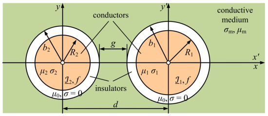
Figure 1.
Two long cylindrical conductors with currents in a conductive medium with non-conductive separating regions—cross-section.
The goal is to find the current density in both conductors. The current in conductor 1 () generates a time-harmonic magnetic field, which induces eddy currents in all conductive regions. In conductor 1, they cause the skin effect, whereas, in conductor 2, they modify the current density resulting from current (proximity effect). The situation is analogical due to eddy currents generated by the current .
The idea of the calculations is as follows: first, the current densities in both conductors due to the skin effect ( and ) are determined. These densities do not take into account the presence of the neighboring conductors. The next step is to calculate eddy currents induced in the conductors due to current in the neighboring conductor. The density of eddy currents induced in conductor 1 due to current in conductor 2 is denoted as . The total current density in conductor 1 is then . Analogical expression can be written for conductor 2. Analytical determination of the current density components under certain simplifications is presented in the following subsections. The simplifications are as follows:
- the wires are placed in a conductive medium, which extends theoretically to infinity,
- the material properties of the wires and the medium are constant,
- the displacement currents are neglected.
Having found the formulas for eddy currents density , the following aspects are investigated:
- what is the distribution of eddy currents density in conductor 2,
- how the skin depth parameters affect the eddy currents density,
- what is the influence of asymmetry in the conductors’ cross-sections,
- what is the influence of insulation thickness,
- how the results are affected in magnetic regions.
As for the total current density and , the following effects are studied:
- the effect of environment conductivity,
- the dependence on frequency,
- the dependence on the distance between the wires.
2.2. Standalone Cylindrical Conductor in Conductive Medium
The first step is considering a single cylindrical conductor placed in a weakly conductive medium (Figure 2). The conductor () has a circular cross-section of radius , electrical conductivity and magnetic permeability . The surrounding region () is a conductive medium of conductivity and permeability . The two regions are separated with a tubular non-conductive and non-magnetic region of external radius . The conductor carries a time-harmonic current of complex r.m.s. value and frequency . The goal is to find out the current density in the conductor as well as the magnetic vector potential in the surrounding medium because it will be necessary for further considerations.
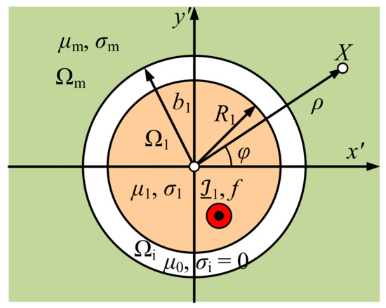
Figure 2.
A long cylindrical conductor () with current in a conductive medium () with the non-conductive separating region ()—cross-section.
It is convenient to introduce a cylindrical coordinate system with -axis located on the axis of the round conductor. Since currents flow only along the -axis, it follows that the current density vector has a -component only, which is independent of the coordinate. Moreover, axial symmetry causes also independence of the angular coordinate so that , where underlining denotes complex phasor. Therefore, the magnetic vector potential can be also assumed to have a -component only, i.e., . In such a case, the Maxwell equations lead to the following equations for the -component of the magnetic vector potential at point :
where is the imaginary unit, and is the angular frequency. These equations can be rewritten as follows:
where
in which
are the skin depths in the cylindrical conductor and the surrounding conductive medium, respectively. Equations (2a)–(2c) have to be completed with the standard interface conditions as well as the Ampère law:
which allows us introducing current to the solutions. The final solutions are as follows:
where and are the modified Bessel functions of order of the first and second kind, respectively, and is any constant. Then, the current density in the round conductor equals:
where superscript “s” indicates that the skin effect is taken into account, and
is the relative current density in the round conductor due to skin effect. Formula (6a) is exactly the same as that for the isolated round conductor in a non-conductive region [35].
Observe that the solution in the surrounding medium can be also rewritten as
where
is an equivalent current, which if placed on the axis of the cylindrical conductor would cause the same effects in the conductive surrounding medium. Equations (7a) and (7b) are used in the next subsection to find the eddy currents density induced in the neighboring conductor ().
2.3. Cylindrical Conductor in Conductive Medium Near a Current Filament
To determine the eddy current density in conductor 2 due to current in conductor 1, the following approach is used: current in conductor 1 generates a time-harmonic magnetic field in its surroundings. When conductor 2 is placed nearby, eddy currents will be induced in it. The density of these eddy currents is denoted as . The magnetic vector potential of the source field is given by Equation (5c), or equivalently—by Equation (7a). The latter is simpler in further considerations; therefore, a filament with current in the conductive medium is used (Figure 3). The conductor () has a circular cross-section of radius , electrical conductivity and magnetic permeability . The two regions are separated with a tubular non-conductive and non-magnetic region of external radius . The filament is placed at a distance of from the conductor’s axis.
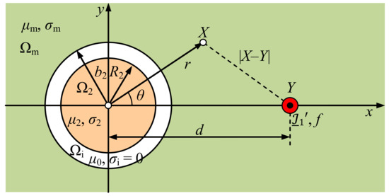
Figure 3.
A long cylindrical conductor () and a parallel current filament in a conductive medium ()—cross-section.
The Maxwell equations lead to the following equations for the -component of the magnetic vector potential at point :
Having found , one can determine the eddy currents induced in the conductor as follows
The total current induced in the conductor equals
It is proportional to because for integrates to 0. This current should be zero (only eddy currents, whose total is zero, are in the conductor); hence, . The remaining constants can be found using conditions for field continuity on boundaries and . The continuity of tangential components of the magnetic field intensity vector leads to the following equations:
The continuity of normal components of magnetic flux density vector yields
where is arbitrary constant resulting from the difference of voltage drops per unit length in the conductor and the surrounding environment.
The further procedure requires representing in terms of coordinates and . By the cosine theorem, it follows that (see Figure 3)
By using formulas 8.406, pos. 3 and 8.407, pos. 1 in 8.531, pos. 2 from [36], the following expansion formula can be derived:
where is any constant and . Therefore,
Using Equations (14a)–(14d) with (12a)–(12c) and (17) after some transformations (see Appendix A for details), one obtains the following expression for coefficient :
where
in which and are the relative magnetic permeabilities of conductor 2 and the surrounding medium, respectively, , and the following notation is introduced:
The details of the derivation are in Appendix A. Other constants and coefficients are omitted here as they are not very important in this paper.
Eddy current density in the round conductor can now be found via Equation (13a), which yields
where superscript “p” stands for the proximity effect, and
is an auxiliary function, which can be interpreted as current density induced in a round conductor placed in the conductive medium by a neighboring filament current placed in a non-conductive cylindrical hollow of radius and expressed in the units of . It depends on several parameters involving dimensions, material properties, and frequency. However, the factual parameters are as follows:
- ,
- ,
- ,
- ,
- ,
- relative permeabilities .
Hence, the independent parameters can be assumed to be
2.4. Special Cases
It is worth considering the case when the insulating regions become extremely thin but still prevent the currents from the round conductors from leaking to the surrounding medium. Then, , and Equation (18b) becomes
so that
Another special case is a non-conductive and non-magnetic medium (, ). Formulas for this case can be obtained by taking the limit . It follows that
so that Equation (18b) yields
Then, by applying Equation (19a) and the following formula (see Equation 8.486, pos. 3 [36]):
The function becomes
When the formula simplifies significantly as follows:
which agrees with that obtained in the literature [2,6,9]. It equals to function defined in [21].
2.5. Total Current Density
The total current density in conductor 2 is the sum of resulting from current in the conductor and resulting from current in conductor 1:
By analogy to Equation (6a), it follows that
and Equation (20a) with (7b) yield
Hence, the total current density in conductor 2 equals
By symmetry, the total current density in conductor 1 equals
It should be realized that the above formulas, although pretty complicated, are the first approximation of the skin and proximity effect only. This is due to the fact that current density is a source of the secondary magnetic field that produces additional eddy currents in conductor 1 (reverse reaction). The currents themselves again induce eddy currents in conductor 2, and so forth. However, these higher-order reactions generate usually very small corrections to the current density in the round conductors and are omitted here. This is discussed in Section 3.5.
3. Results and Discussion
3.1. Comparison with FEM and BEM Results
The first step in presenting results is checking whether the solution given by Equations (20a) and (20b) is correct. To do this, the computations for several cases are performed using the equations as well as two numerical methods: finite element method (FEM) and boundary element method (BEM). The FEM analysis is done using FEMM software (version 4.2, 64-bit 21Apr2019 by David Meeker, MA, USA, http://www.femm.info/wiki/HomePage) with a suitably fine mesh of first-order triangular finite elements. In BEM calculations, parabolic boundary elements with constant field approximation are used (i.e., the geometry is approximated with parabolic curvilinear elements to reflect exactly the shape of the round conductor, whereas the field approximations throughout an element are constant). The computations are performed for a copper wire (, ) at such a frequency for which the skin depth equals . The thickness of insulation is assumed zero (), and the distance to the filament is . Four types of surrounding medium are considered:
- non-conductive and non-magnetic medium;
- non-magnetic conductive () medium;
- non-conductive magnetic () medium;
- conductive () and magnetic () medium.
The values of vs. for these four cases are presented in Figure 4 (modulus) and Figure 5 (argument). The results obtained via Equation (20b) (solid lines) agree very well with those by BEM (circles), but surprisingly there are some discrepancies with those by FEM (dots). The discrepancy occurs only when is non-zero (red and cyan traces). To check which results are correct, also BEM calculations are performed, and a full agreement with Equation (20b) is obtained. Hence, FEM results are incorrect for the conductive surrounding region. Further analysis has revealed that the reason is the way of modeling the infinite surrounding region in FEMM software: the Kelvin transformation is used, which is true if the field at infinity can be modeled with the Laplace equation. However, when the medium is conductive, it is no longer true, and therefore some discrepancies arise. Hence, it follows that Equation (20b) agrees with the results obtained via other methods.
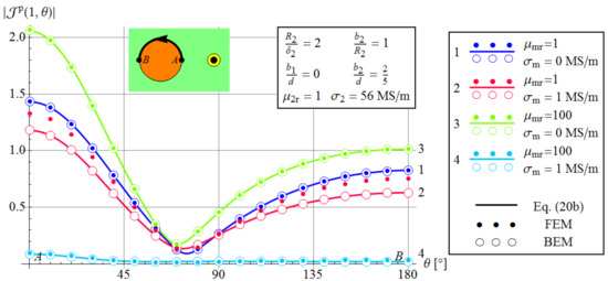
Figure 4.
The modulus of on the surface of conductor 2 due to current filament for various material parameters of the surrounding medium at constant remaining parameters (see the middle inset); the left inset shows the plotting path on the cross-section of the configuration.
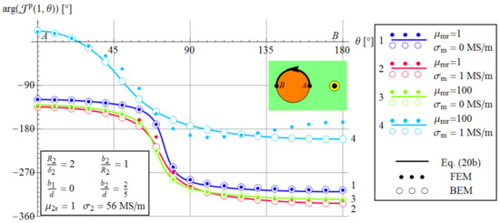
Figure 5.
The argument of on the surface of conductor 2 due to current filament for various material parameters of the surrounding medium at constant remaining parameters (see the left bottom inset); the green inset shows the plotting path on the cross-section of the configuration.
3.2. The Influence of Various Parameters on Eddy Current Density
The density of eddy currents due to the proximity effect is given by Equation (20a), in which function defined in Equation (20b), is used. Below, function is tested with respect to particular parameters, and a short discussion for each effect is provided.
3.2.1. Current Density Distribution
Figure 6 and Figure 7 present vs. and vs. , respectively, on the surface of the conductor 2 for six various values of in the case of non-magnetic medium and tangent conductors. Trace 1 corresponds to a non-conductive medium. It agrees with that presented in the graph in Section 3.2.4. [21]. As the skin depth in the medium decreases, the maxima of decrease, too, so that the distribution of becomes flatter. This effect is related to weakening the field due to losses in the conductive medium as well as with the phase lag in the surrounding conductive medium, which is visible in Figure 7.
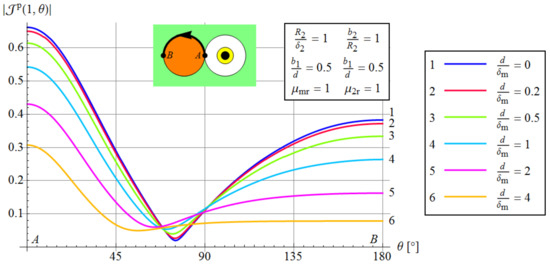
Figure 6.
The distribution of eddy currents density on the conductor surface: the modulus of on the surface of conductor 2 due to current in conductor 1 for various skin depths in the surrounding medium at constant remaining parameters (see inset in the right top corner); the top center inset shows the plotting path on the cross-section of the configuration.
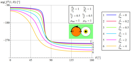
Figure 7.
The distribution of eddy currents density on the conductor surface: the argument of on the surface of conductor 2 due to current in conductor 1 for various skin depths in the surrounding medium at constant remaining parameters (see the inset in the top right corner); the inset above the traces shows the plotting path on the cross-section of the configuration.
Figure 8 presents vs. in conductor 2 for the same cases as in Figure 6 and Figure 7. Trace 1 corresponds to a non-conductive medium, and it agrees with traces 1 and 3 presented in the graph in Section 3.2.3. [21]. As the skin depth in the medium decreases, the decreases, too, so that the influence of the proximity effect becomes smaller.
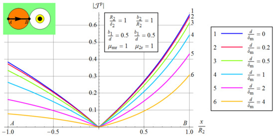
Figure 8.
The distribution of eddy current density across the wire: the modulus of along the symmetry axis in conductor 2 due to current in conductor 1 for various skin depths in the surrounding medium at constant remaining parameters (see the middle inset); the leftmost inset shows the plotting path on the cross-section of the configuration.
3.2.2. The Effect of Skin Depth
Figure 9 shows at the point on conductor 2 closest to conductor 1 vs. for various and constant remaining parameters for non-magnetic regions. The smaller the skin depth in the surrounding medium, the smaller are the induced eddy currents. The effect is the stronger the smaller the skin depth in conductor 2.
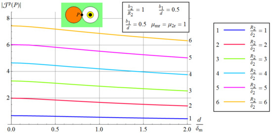
Figure 9.
The effect of skin depth in the surrounding medium for various skin depths in the wire: the modulus of at the point closest to conductor 1 (see the leftmost inset) due to current in conductor 1 vs. ratio for various skin depths in conductor 2 at constant remaining parameters (see the middle inset).
3.2.3. The Effect of Size Asymmetry
Figure 10 shows at the point on conductor 2 closest to conductor 1 vs. for various and for non-magnetic regions. The values of are the greater the smaller the values of (i.e., the larger is ). As the skin depth in the surrounding medium increases, the values of decrease.
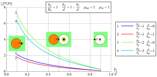
Figure 10.
The effect of asymmetry in conductors’ cross-sections: the modulus of at the point closest to conductor 1 due to current in conductor 1 vs. ratio for various skin depths in conductor 2 and ratios (see the top inset); the distance between the conductors is assumed ; therefore, in this case.
3.2.4. The Effect of Insulation Thickness
Figure 11 shows at the point on conductor 2 closest to conductor 1 vs. relative thickness of insulation (, where ) for various and for non-magnetic regions and constant and . The effect is the greater the smaller the skin depths in the conductor and medium. For a non-conductive medium, the insulation thickness has no effect.
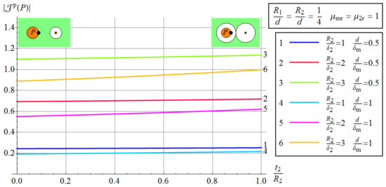
Figure 11.
The effect of insulation thickness: the modulus of at the point closest to conductor 1 (see the top insets) due to current in conductor 1 vs. thickness to radius ratio for various skin depths in conductor 2 and the medium at constant remaining parameters (see the right top inset).
3.2.5. The Effect of The Magnetic Medium
Figure 12 shows at the point on conductor 2 closest to conductor 1 vs. for various and constant remaining material parameters. It follows that at small enough distances, the density of eddy currents increases as the environment permeability increases, but for larger distances, the effect is inverse. An increase in permeability lowers the skin depth, making stronger the attenuation of the field in the medium. This is best visible with trace 6. An interesting thing is that trace 4 indicates the strongest action on conductor 2. This is related to the small conductivity of the medium (weak attenuation).
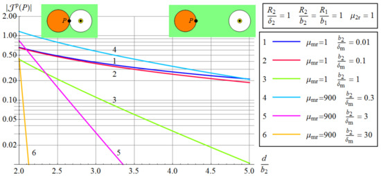
Figure 12.
The effect of magnetic medium: the modulus of at the point closest to conductor 1 (see the top insets) due to current in conductor 1 vs. ratio for various skin depths in conductor 2 and the environment permeability ( affects ).
3.3. Symmetrical Twin Line—Numerical Results and Discussion
In this subsection, a twin line is considered. The wires are assumed identical and made of copper (, , , ), with a negligibly small thickness of insulation (, ) and distance between their axes equal to , where is the gap between their closest points. The remaining parameters (, , , ) are subject to change. Two cases are considered: the same currents and opposing currents. In all cases, the total current density is divided by DC current density as follows:
3.3.1. Comparison with FEM and BEM
Figure 13 and Figure 14 present the distribution of the relative current density in conductor 2 for same and opposing currents and arbitrary parameters given in the framed insets. Four cases are considered: (1) same currents in a non-conductive medium; (2) same currents in the medium of conductivity equal to 1 MS/m; (3) opposing currents in a non-conductive medium; (4) opposing currents in the medium of conductivity equal to 1 MS/m.
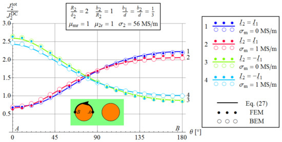
Figure 13.
The effect of conductance of the surrounding medium for same and opposing currents—distribution of the magnitude of relative current density on the surface of conductor 2, as shown in the bottom inset; copper wires with the gap between them equal to their radius.
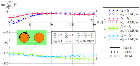
Figure 14.
The effect of conductance of the surrounding medium for same and opposing currents—distribution of the argument of relative current density on the surface of conductor 2, as shown in the left inset; copper wires with the gap between them equal to their radius.
In addition to theoretical calculations via Equation (27), the FEM and BEM analysis is used in a similar way as in Section 3.1. The wires are made of copper, the gap between the wires is equal to their radius, and the medium is non-magnetic. It follows that the non-magnetic conductive medium weakens the proximity effect. The BEM results (circles) are close to that of Equation (27), but there are small discrepancies. They are due to the fact that Equation (27) does not take into account higher reactions (the induced eddy currents also induce eddy currents in conductor 1, and so forth—see [21]). The FEM results are the same as BEM results in the case of a non-conductive medium, but they are clearly different for a conductive medium. As mentioned in Section 3.1, this is caused by the way in which the open boundary problem is modeled in FEMM software.
3.3.2. The Effect of Environment Conductivity and The Gap between The Wires
Figure 15 presents across that diameter of conductor 2, which is parallel to the symmetry axis intersecting the conductors. Three values of ratio and two values of environment conductivity are taken into account. An increase in the conductivity of the medium weakens the proximity effect because the induced currents due to the current in the neighboring wire are smaller (electromagnetic screening by the conductive medium). The effect is, however, noticeable for high enough environment conductivity or large enough gap between the wires.
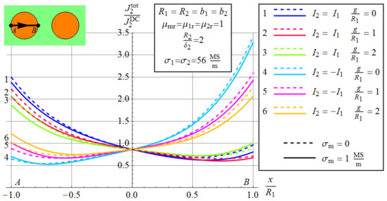
Figure 15.
The effect of conductivity of the surrounding medium and the effect of the distance between the conductors: the values of the magnitude of the relative current density in conductor 2 across its diameter (see the leftmost inset) for various gaps between the conductors; traces 1–3 are for same currents, traces 4–6 are for opposing currents; dashed lines are for non-conductive medium, whereas solid lines are for ; the remaining parameters are given in the middle inset.
3.3.3. The Effect of Frequency and Conductivity of The Medium
Figure 16 presents across that diameter of conductor 2, which is parallel to the symmetry axis intersecting the conductors. Three values of frequency (expressed as ratio) and two values of environment conductivity are considered. An increase in frequency strengthens the proximity effect. An increase in environment conductivity weakens the proximity effect due to the screening activity of the medium.
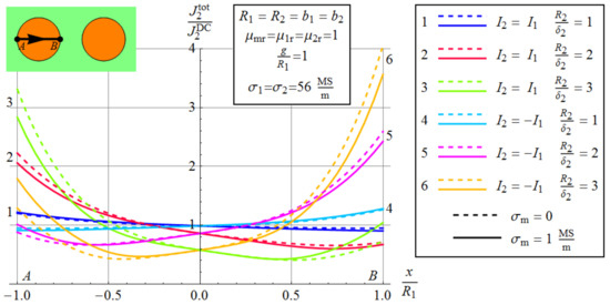
Figure 16.
The effect of frequency and conductivity of the medium: the values of the magnitude of the relative current density in conductor 2 across its diameter (see the leftmost inset) for various ratios (proportional to ); traces 1–3 are for same currents, traces 4–6 are for opposing currents; dashed lines are for non-conductive medium, whereas solid lines are for ; the remaining parameters are given in the middle inset.
3.4. Implications
Equations (6a) and (6b) show that the skin effect in a standalone round conductor placed in a conductive medium is the same as in for non-conductive medium. Figure 4, Figure 5, and Figure 9 indicate that the eddy currents induced in a round conductor due to a neighboring current filament are smaller if the surrounding medium is conductive. This result is intuitively clear because the conductive medium acts as an electromagnetic screen. For non-magnetic medium, the change is noticeable for conductivity values much larger than 10 S/m. Figure 13, Figure 14, Figure 15 and Figure 16 also confirm this. To see it better, the following indicator is introduced:
which is the percentage change in value in relation to this value for the non-conductive medium. Figure 17 shows vs. for copper wires and various other parameters. It follows that noticeable changes can be observed for S/m. Hence, the effect of surrounding soil or sea water on the proximity effect in a twin line with round conductors can be neglected because the relative changes in current density are below 0.01%. However, this does not mean the impedances will not be changed to a larger degree because of eddy currents induced in the conductive medium. They are a source of additional power losses, so the effect of lowering the proximity effect in the wires may be diminished by an increase of power losses in the conductive medium. Moreover, the results do not take into account the complex permittivity of the surrounding medium, which may affect the results for specific values of higher frequencies. The above aspects will be subject to further investigations. It is also to remember that the results are obtained by neglecting the displacement currents, which can have a certain effect in case of very high frequencies and wires placed in a very weakly conductive medium.
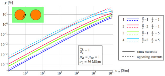
Figure 17.
Relative change in current density in the closest point (point in the left top inset) vs. conductivity of the medium for various parameters.
3.5. Limitations and Error Estimation
Finally, it is necessary to indicate that Equation (27) is an approximation of the true solution for a twin line with round conductors. It should be realized that eddy currents of density induce eddy currents in conductor 1, which generate additional eddy currents in conductor 2, and so forth. This is presented in Figure 18. Let us observe that each successive reaction is much weaker than the previous one because it can be regarded as a result of two opposite currents. For example, the light brown arrows in wire 2 (solid and dashed) represent eddy currents and generate much weaker reaction 2 in wire 1 (short black arrows equal to differences between orange and brown arrows, depicting reactions to the light brown solid and dashed arrows). These higher-order reactions are not included in Equation (27). However, usually, they are very small (see [21], where these reactions were found in the case of the non-conductive surrounding region).
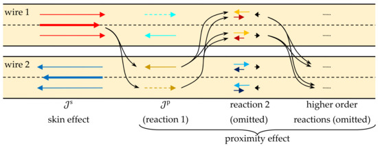
Figure 18.
Schematic view of interactions between currents in the wires. The current in wire 1 (thick red arrow) induces eddy currents in wire 1 (the skin effect—red arrows) and in wire 2 (the first approximation of the proximity effect—light brown arrows of opposite direction because the induced current equals zero). These eddy currents in wire 2 induce eddy currents in wire 1 (orange and brown arrows); the orange ones originate from the current symbolize with a light brown solid lines, whereas the brown ones originate from the current symbolize with light brown dashed line. Reaction 2 (short black arrows) is then the difference between the orange and brown arrows and, therefore, is much weaker than reaction 1. The higher-order reactions arise in a similar way and quickly tend to zero.
To estimate the error due to the omitted higher reactions, let us substitute wire 2 (where currents of density are induced, Equation (20a)) with two filaments, A and B, with opposite currents , as shown in Figure 19, where
Factor originates from the fact that the total induced current in wire 2 equals 0, so approximately half of the cross-section carries current , whereas the other half carries the return current. Then, according to Equation (20a), such two filaments induce eddy currents in wire 1 as follows
The maximum density occurs in the point nearest to wire 2, i.e., when and . In the nonmagnetic case () with thin insulation (, ), it follows that the maximum of equals
where . The above value overestimates the second reaction because of the oversized current in extremely close filament A and the closest points taken. Moreover, the successive higher reactions have different phases so that they cancel partially (the phase difference is around 90° for points on wire surface in case of weakly conductive medium). This means that the error in current density in wire 1 is not greater than , but usually it is much less. Further simplification can be obtained by considering the case of weak skin effect (, ) and non-conductive medium (). By using some mathematical effort (limits, power series expansion, geometrical series summation), the following expression can be obtained:
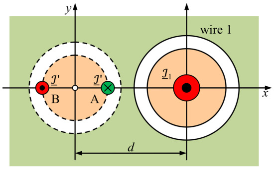
Figure 19.
Wire 2 with eddy currents of density due to current is replaced with two current filaments A and B with current ; these two filaments induce eddy currents in wire 1.
This expression can serve as maximum error estimation in current density in the case of nonmagnetic wires with thin insulation. It is relatively simple in form and involves basic dimensions as well as the skin depths of the wires. When the medium is conductive, the error is smaller due to the attenuation introduced by the medium. When the skin effect in the wires is larger, the error is also smaller because of the phase lag in the wires, which makes partial cancellation of the currents. This is shown in Figure 20.
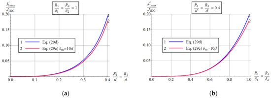
Figure 20.
Error estimation of the solution; the true error is much less due to much overestimated action of filament A and partial cancellation of the successive reactions: (a) error vs. for constant ; (b) error vs. for constant .
The higher-order reactions may have a noticeable influence in the case of very small gaps at higher frequencies, as visible in Figure 13 and Figure 14, where some differences between Equation (27) and BEM results can be observed. Especially two cases must be mentioned: (i) when the conductivity of the medium is rather high (at least 1% of that for wires); (ii) when the magnetic permeabilities of the regions differ considerably. Another limitation is the fact that the whole surrounding region is assumed conductive and homogeneous, i.e., no ground surface is taken into account.
4. Conclusions
Based on the above considerations, the following conclusions can be formulated:
- The eddy currents density in the round conductors placed in the non-magnetic conductive medium is decreased compared to the same conductor in the non-conductive and non-magnetic medium due to the screening effect of the medium. This results in decreasing the proximity effect.
- If the conductors are placed in the magnetic and non-conductive medium, the proximity effect is enlarged.
- For the conductive and magnetic medium, the proximity effect is decreased in a larger degree compared to the case of a non-magnetic medium of the same conductivity.
- For copper conductors placed in soil or sea water, the change in current density distribution is very small, usually below 0.01%.
- Further investigations can be focused on tubular conductors and groups of conductors as well as on their impedances; also the boundaries of the medium can be taken into account.
Author Contributions
conceptualization, P.J. and Z.P.; methodology, P.J. and Z.P.; software, P.J.; validation, Z.P., D.K., and T.S.; formal analysis, P.J and Z.P.; writing—original draft preparation, P.J.; writing—review and editing, D.K. and T.S.; visualization, P.J.; supervision, P.J. All authors have read and agreed to the published version of the manuscript.
Funding
This research received no external funding. The APC was funded by the Czestochowa University of Technology.
Conflicts of Interest
The authors declare no conflict of interest.
Appendix A
To ensure a satisfying Equations (14a)–(14d) for any the corresponding coefficients of for each must be equal. For the following equations are obtained:
Taking into account that (see Equation (13b)), it follows that
For the following equations are obtained
Equations (A6) and (A8) yield
where functions and are defined by Equations (19a) and (19b). Combining Equations (A7) and (A9) leads to
Substituting Equation (A10) for and Equation (A11) for in Equation (A12) leads to some transformations in Equations (18a) and (18b). During the transformations, the following equation is used (see [37] 9.6.15 + 9.6.26):
References
- Maxwell, J.C. A Treatise of Electricity and Magnetism; McMillan and Co.: London, UK, 1873; Volume II, Article 689. [Google Scholar]
- Manneback, C. An integral equation for skin effect in parallel conductors. J. Math. Phys. 1922, 1, 123–146. [Google Scholar] [CrossRef]
- Dwight, H.B. Proximity effect in wires and thin tubes. Trans. Am. Inst. Electr. Eng. 1923, 42, 850–859. [Google Scholar] [CrossRef]
- Tegopoulos, J.A.; Kriezis, E.E. Eddy current distribution in cylindrical shells of infinite length due to axial currents. Part I: Shells of one boundary. IEEE Trans. Power Appar. Syst. 1981, 90, 1278–1286. [Google Scholar] [CrossRef]
- Tegopoulos, J.A.; Kriezis, E.E. Eddy current distribution in cylindrical shells of infinite length due to axial currents. Part II: Shells of finite thickness. IEEE Trans. Power Appar. Syst. 1981, 90, 1287–1294. [Google Scholar] [CrossRef]
- Piątek, Z. Method of calculating eddy currents induced by the sinusoidal current of the parallel conductor in the circular conductor. ZN Pol. Śl. Elektr. 1981, 75, 137–150. [Google Scholar]
- Piątek, Z. Self and mutual impedances of a finite length gas-insulated transmission line (GIL). Electr. Power Syst. Res. 2007, 77, 191–201. [Google Scholar] [CrossRef]
- Piątek, Z. Impedances of Tubular High Current Busducts; Polish Academy of Sciences: Warsaw, Poland, 2008.
- Filipović, D.; Dlabač, T. Closed Form Solution for the Proximity Effect in a Thin Tubular Conductor Influenced by a Parallel Filament. Serb. J. Electr. Eng. 2010, 7, 13–20. [Google Scholar]
- Dlabač, T.; Filipović, D. Integral equation approach for proximity effect in a two-wire line with round conductors. Tech. Vjesn. 2015, 22, 1065–1068. [Google Scholar] [CrossRef]
- Jabłoński, P. Cylindrical conductor in an arbitrary time-harmonic transverse magnetic field. Przegląd Elektrotech. 2011, 87, 49–53. [Google Scholar]
- Rolicz, P. Eddy currents generated in a system of two cylindrical conductors by a transverse alternating magnetic field. Electr. Power Syst. Res. 2009, 79, 295–300. [Google Scholar] [CrossRef]
- Jabłoński, P. Approximate BEM analysis of time-harmonic magnetic field due to thin-shielded wires. Pozn. Univ. Technol. Acad. J. Electr. Eng. 2012, 69, 57–64. [Google Scholar]
- Piątek, Z.; Baron, B.; Jabłoński, P.; Kusiak, D.; Szczegielniak, T. Numerical method of computing impedances in shielded and unshielded three-phase rectangular busbar systems. Prog. Electromagn. Res. B 2013, 51, 135–156. [Google Scholar] [CrossRef]
- Coufal, O. Current density in two solid parallel conductors and their impedance. Electr. Eng. 2014, 96, 287–297. [Google Scholar] [CrossRef]
- Freitas, D.; das Neves, M.G.; Almeida, M.E.; Machado, V.M. Evaluation of the Longitudinal Parameters of an Overhead Transmission Line with Non-Homogeneous Cross Section. Electr. Power Syst. Res. 2015, 119, 478–484. [Google Scholar] [CrossRef]
- Riba, J.R. Calculation of AC to DC resistance ratio of conductive nonmagnetic straight conductors by applying FEM simulations. Eur. J. Phys. 2015, 36, 055019. [Google Scholar] [CrossRef][Green Version]
- Capelli, F.; Riba, J.R. Analysis of Equations to calculate the AC inductance of different configurations of nonmagnetic circular conductors. Electr. Eng. 2017, 99, 827–837. [Google Scholar] [CrossRef]
- Riba, J.R.; Capelli, F. Calculation of the inductance of conductive nonmagnetic conductors by means of finite element method simulations. Int. J. Electr. Educ. 2018, 13, 230–252. [Google Scholar]
- Pagnetti, A.; Xemard, A.; Pladian, F.; Nucci, C.A. An improved method for the calculation of the internal impedances of solid and hollow conductors with inclusion of proximity effect. IEEE Trans. Power Deliv. 2012, 27, 2063–2072. [Google Scholar] [CrossRef]
- Jabłoński, P.; Szczegielniak, T.; Kusiak, D.; Piątek, Z. Analytical-numerical solution for the skin and proximity effects in two parallel round conductors. Energies 2019, 12, 3584. [Google Scholar] [CrossRef]
- Benato, R.; Paoluci, A. EHV AC Undergrounding Electrical Power. Performance and Planning; Springer: London, UK, 2010. [Google Scholar]
- Katsube, T.J.; Klassen, R.A.; Das, Y.; Ernst, R.; Calvert, T.; Cross, G.; Hunter, J.; Best, M.; DiLabio, R.; Connell, S. Prediction and validation of soil electromagnetic characteristics for application in landmine detection. In Detection and Remediation Technologies for Mines and Mine Like Targets VIII. Proceedings of SPIE Vol. 5089, AeroSense 2003, Orlando, FA, USA, 11 September 2003; Harmon, R.S., Holloway, J.H., Jr., Broach, J.T., Eds.; Society of Photo-Optical Instrumentation Engineers (SPIE): Washington, DC, USA, 2003; pp. 1219–1230. [Google Scholar] [CrossRef]
- Zdeb, M.; Papciak, D.; Zamorska, J. An assessment of the quality and use of rainwater as the basis for sustainable water management in suburban areas. E3S Web Conf. 2018, 45, 00111. [Google Scholar] [CrossRef]
- Tyler, R.H.; Boyer, T.P.; Minami, T.; Zweng, M.M.; Reagan, J.R. Electrical conductivity of the global ocean. Earth Planets Space 2017, 69, 156. [Google Scholar] [CrossRef] [PubMed]
- Pollaczek, F. Über das Feld einer unendlich langen wechsel-stromdurchflossenen Einfachleitung. Elektr. Nachr. Tech. 1926, 3, 339–360. [Google Scholar]
- Machado, V.M.; da Silva, J.F.B. Series-impedance of underground transmission systems. IEEE Trans. Power Deliv. 1988, 2, 417–424. [Google Scholar] [CrossRef]
- Machado, V.M.; da Silva, J.F.B. Series-impedance of underground cable systems. IEEE Trans. Power Deliv. 1988, 3, 1334–1340. [Google Scholar] [CrossRef]
- Tsiamitros, D.A.; Christoforidis, G.C.; Papagiannis, G.K.; Labridis, D.P.; Dokopoulos, P.S. Earth conduction effects in systems of overhead and underground conductors in multilayered soils. IEEE Proc. Gener. Transm. Distrib. 2006, 153, 291–299. [Google Scholar] [CrossRef]
- Yin, Y.; Dommel, H.W. Calculation of frequency-dependent impedances of underground power cables with finite element method. IEEE Trans. Magn. 1989, 25, 3025–3027. [Google Scholar] [CrossRef]
- Machado, V.M. FEM/BEM hybrid method for magnetic field evaluation due to underground power cables. IEEE Trans. Magn. 2010, 46, 2876–2879. [Google Scholar] [CrossRef]
- Machado, V.M.; Almeida, M.E.; das Neves, M.G. Accurate magnetic field evaluation due to underground power cables. Eur. Trans. Electr. Power 2009, 19, 1153–1160. [Google Scholar] [CrossRef]
- Budnik, K.; Machczyński, W. Magnetic field of underground cables. Elektryka 2010, 3, 7–17. [Google Scholar]
- Brito, A.I.; Machado, V.M.; Almeida, M.E.; das Neves, M.G. Skin and Proximity Effects in the Series-Impedance of Three-Phase Underground Cables. Electr. Power Syst. Res. 2016, 130, 132–138. [Google Scholar] [CrossRef]
- Moon, P.; Spencer, D.E. Foundations of Electrodynamics; David Van Nostrand Company, Inc.: New York, NY, USA, 1960. [Google Scholar]
- Gradshteyn, I.S.; Ryzhik, I.M. Tables of Integrals, Sums, Series and Products, 17th ed.; Elsevier Academic Press: Cambridge, MA, USA, 2007. [Google Scholar]
- Abramowitz, M.; Stegun, I.A. Handbook of Mathematical Functions with Formulas, Graphs, and Mathematical Tables; Applied Mathematics Series 55; National Bureau of Standards: Washington, DC, USA, 1972.


Publisher’s Note: MDPI stays neutral with regard to jurisdictional claims in published maps and institutional affiliations. |
© 2020 by the authors. Licensee MDPI, Basel, Switzerland. This article is an open access article distributed under the terms and conditions of the Creative Commons Attribution (CC BY) license (http://creativecommons.org/licenses/by/4.0/).