Two-Stage Optimal Microgrid Operation with a Risk-Based Hybrid Demand Response Program Considering Uncertainty

Abstract

Owing to the increasing utilization of renewable energy resources, distributed energy resources (DERs) become inevitably uncertain, and microgrid operators have difficulty in operating the power systems because of this uncertainty. In this study, we propose a two-stage optimization approach with a hybrid demand response program (DRP) considering a risk index for microgrids (MGs) under uncertainty. The risk-based hybrid DRP is presented to reduce both operational costs and uncertainty effect using demand response elasticity. The problem is formulated as a two-stage optimization that considers not only the expected operation costs but also risk expense of uncertainty. To address the optimization problem, an improved multi-layer artificial bee colony (IML-ABC) is incorporated into the MG operation. The effectiveness of the proposed approach is demonstrated through a numerical analysis based on a typical low-voltage grid-connected MG. As a result, the proposed approach can reduce the operation costs which are taken into account uncertainty in MG. Therefore, the two-stage optimal operation considering uncertainty has been sufficiently helpful for microgrid operators (MGOs) to make risk-based decisions.

1. Introduction

In a smart-grid environment, distributed energy resources (DERs), such as renewable energy, have gained more attention than traditional power generation units owing to the increasing trend to address environmental concerns [1,2]. Some of the most widely used renewable energy resources are wind turbine (WT) and photovoltaic (PV) systems because of the feasibility of existing related technologies. However, these forms of DERs are dependent on fluctuations and the unpredictive nature of wind and solar resources. Since the difficulty in managing distributed uncertainties by conventional power systems, microgrids (MGs) that can usefully control DERs have been introduced as a new concept [3]. MGs manage a cluster of loads and DERs, operating as a control to offer power locally. MGOs should be able to confirm the reliability of systems considering uncertain risk indices. In this regard, the accurate evaluation of MGs is a challenging task due to the uncertainties inherent in renewable energy. Moreover, methods are needed to mitigate the effects of uncertainty when scheduling optimal operations [4]. In this situation, using flexible energy, such as demand response (DR), can provide the required demand control for the system and can be used reliably in a relatively short time under the same conditions [5]. Thus, the DR program (DRP) for power systems is expected to advance steadily [6]. This is because power system infrastructure is focused on both stability and economics, and the DRP is a flexible and inexpensive resource for operating a system. MGOs can use the DRP to reduce the peak load, save on the power reserve, and ensure power reliability. The operators can also encourage customers to use less power during periods when demand reduction is required owing to uncertainties. Thus, customers engage in contracts with MGOs to reduce demand when requested, and MGOs offer incentive costs to customers that reflect the amount of demand reduced, enabling contracts to be maintained.

Various approaches have been used recently to address uncertain problems inherent in MG operation. To minimize operational costs under a deterministic and probabilistic environment, a stochastic approach for MG operation using energy storage system (ESS) was proposed in Reference [7]. In Reference [8], optimal planning for interconnected MGs under uncertainty in large-scale distribution systems was presented to improve reliability and economics. Further, to improve system operation and management efficiency, a stochastic resource planning strategy for MGs was introduced in Reference [9] to optimally manage resources required for both the generation and demand sides. In Reference [10], both the power generation of each unit and the exchange with upstream networks were assessed through the optimal operation of MGs. Artificial intelligence algorithms were used to forecast wind speeds and optimal set volumes for DERs, and ESS capacity was determined based on forecasted data to optimize the total operating costs by Motevasel et al. [11]. Moreover, a probabilistic methodology of uncertainties caused by wind and solar generation and load consumption for estimating spinning reserve requirement was presented in Reference [12]. The DRP was considered to control the frequency of a smart MG with renewable generation, and mixed-integer linear programming was used to solve the proposed model for wind-power generation under uncertainty [13]. A stochastic planning approach was suggested to model the probabilistic behavior of wind and DRs in an energy market [14]. The authors in Reference [15] studied the effects of demand-side management of appliances on the reliability, loss, and voltage profiles of power systems, and customer comfort was also considered. Using a risk-based stochastic optimization framework, the minimum required ESS to secure the desired voltage stability margin for distribution systems was computed by Jalali et al. [16]. The authors in Reference [17] presented a flexible risk control strategy with an ESS to help remedy the removal of line overload in post-contingency situations. To minimize operating costs of MGs using the genetic algorithm, the optimal energy and power capacity of energy storage systems were determined [18]. The operational costs of MGOs were reduced by selling remaining energy at a high load level by Samadi et al. [19]. This study addressed a daily power prediction module to provide MGs with solar power output data for DER scheduling. However, the reserve for compensating wind and PV power fluctuations was not considered within the daily DER schedule. The authors in Reference [20] solved the optimal power flow through particle swarm optimization on a system of MGs with WT. To date, several important studies on realizing optimal operation for MG systems accompanied with uncertainties have been conducted [6,7,8,9,10,11,12,13,14,15,16,17,18,19,20]. However, the risk strategy of uncertainty was mostly not considered when computing the optimization problem. Although uncertainty is inevitable in MG operation, few studies have considered risk scenarios. The DRP can be used in various approaches to improve system reliability and reduce operational costs, but it has generally been used as a single solution. Therefore, it is necessary not only to operate MGs considering risk strategy but also to utilize the hybrid DRP according to the risk-averse tendency of MGOs.

In this study, we present a two-stage optimization model for optimal operation in grid-connected MG considering the DRP with a risk strategy. Load, PV, and WT are considered as uncertainty variables, and each unit is modeled through a certain probability distribution function (PDF). Monte Carlo simulation and k-means clustering are used implement the scenarios. The risk-based hybrid demand response program (RH-DRP) is proposed to reduce risk-based operational costs by determining optimal DR volume configuration in accordance with risk aversion parameter. In the two-stage optimization problem, the expected operational costs are calculated in first-stage and then, the risk-based operational costs are determined via the conditional value at risk (CVaR) index in second-stage. This is successfully addressed using the improved multi-layer artificial bee colony (IML-ABC), a modified conventional ABC algorithm that improves convergence speed.

The main contributions of this paper can be summarized as follows:

• The proposed two-stage optimization is developed to calculate the risk-based operation costs while considering uncertainty based on scenarios. It assists MGOs make decisions from more additional degree of freedom.
• The effectiveness of applying the RH-DRP is evaluated in terms of the total risk-based operation costs reduction, and the superiority of the RH-DRP is demonstrated via comparison analysis with different DR strategies.
• The IML-ABC shows better performance in searching for optimal solutions in comparison with the different optimal algorithms. Furthermore, it achieves simulation time reduction with the rapid convergence speed and can be applied for a variety of optimization problems.

The remainder of this paper is organized as follows. Section 2 introduces uncertainty modeling for WT, PV, and load. Section 3 shows the proposed RH-DRP strategy, and Section 4 provides formulations for the risk-based two-stage optimization problem. Section 5 presents the solution method used by the IML-ABC algorithm and summarizes the overall process of the optimal operation approach. Section 6 presents the numerical analysis results, and, finally, Section 7 concludes the paper.

2. Uncertainty Modeling for Microgrid Operation

2.1. Uncertainty Modeling

In this study, a probabilistic model is used to minimize operating costs in a microgrid considering uncertainty. Accurate prediction is not possible due to the stochastic behavior of wind and solar irradiance and it is always related to the uncertainty error of the plan for the next day. Thus, to consider more realistic compliance, we use probability density function (PDF) to model the behavior of wind, solar, and load to achieve optimal results considering uncertainties.

2.1.1. Wind Generation Modeling

The Weibull PDF has been regularly used to model wind speed at a forecasted time [21] and can be expressed as

$$PD{F}_w(v)=\left(\frac{d}{C}\right){\left(\frac{v}{C}\right)}^{d-1} \exp \left[-{\left(\frac{v}{C}\right)}^d\right],$$

(1)

where d and C are the factors that characterize the Weibull PDF and determine the shape and scale, respectively, and v is the wind speed.

$$P_w(v)=\{\begin{array}{c}0\\ P_r\times \frac{(v_{wind}-v_{ci})}{(v_r-v_{ci})}\\ P_r\\ 0\end{array}\hspace{1em}\hspace{1em}\begin{array}{c}{v}_{wind}<v_{ci}\\ v_{ci}\le v_{wind}<v_r\\ v_r\le v_{wind}<v_{co}\\ v_{co}\le v_{wind}\end{array}.$$

(2)

The output power of WT can be calculated using the WT power curve parameters: where P_r, v_ci, v_r, and v_co are the rated power, cut-in speed, rated speed, and cut-off speed of the WT, respectively.

2.1.2. Solar Generation Modeling

Solar generation output depends on the amount of sun irradiance. Forecasted solar power generation is commonly calculated using the beta PDF expressed as follows [22]:

$$PD{F}_B(si)=\{\begin{array}{c}\frac{\Gamma (a+b)}{\Gamma (a)\Gamma (b)} \times s{i}^{(a-1)}\times {(1-si)}^{(b-1)}\\ 0\end{array} \begin{array}{c}0\le si\le 1 , a\ge 0 , b\ge 0\\ otherwise\end{array},$$

(3)

$$a=\frac{{\mu }_s\times b}{1-{\mu }_s},$$

(4)

$$b = (1-{\mu }_s)\times \left(\frac{{\mu }_s\times (1+{\mu }_s)}{{\sigma }_s{}^2}-1\right).$$

(5)

Here, si is the amount of solar irradiance (kWh/m²), and a and b are the beta PDF parameters that can estimate the mean (μ_s) and standard deviation (σ_s) according to the solar irradiance data, respectively.

Depending on the characteristics of the PV panels, solar irradiance can be converted to solar power by

$$P_{PV}(si)={\eta }_{pv} \times A_{pv} \times si,$$

(6)

where P_pv(si) represents the amount of PV output power for irradiance, η_pv is the efficiency of the PV panels, and A_pv is the total surface area of the PV panels.

2.1.3. Load Modeling

Uncertainty in load consumption caused by the stochastic behavior of power consumers can be modeled as a typical probability function with a normal PDF [23].

$$PD{F}_n(load)=\frac{1}{\sqrt{2\pi }\times {\sigma }_l}\exp \left(\frac{{(P_{load}-{\mu }_l)}^2}{2{\sigma }_l{}^2}\right),$$

(7)

where P_load is load demand, and μ_l and σ_l are the mean value and standard deviation of the load, respectively.

2.2. Scenario Generation and Reduction

In stochastic cases, the high occurrence probability has the most effect on decision makers. However, high probability situations do not always arise, whereas low probability situations may occur at any time [24]. If the low probability scenario has a critical effect, it should be considered in the decision making. The MGO would then be confronted with a problem with uncertainty, such as renewable power and load consumption in MG operation. Our study conducted scenario modeling using Monte Carlo simulations to analyze various scenarios, including the risk situation for all low probabilities with a critical effect. The generated scenarios for the load demand (${\varphi }_{Ln}^{}$) and power generation of WT (${\varphi }_{WTn}^{}$) and PV (${\varphi }_{PVn}^{}$) are expressed as follows:

$${\varphi }_{Ln}^{}=(L_n,{\psi }_{Ln}^{}),\hspace{1em}\hspace{1em}\hspace{1em}{\displaystyle \sum _1^N{\psi }_{Ln}^{}=1},$$

(8)

$${\varphi }_{WTn}^{}=(W{T}_n,{\psi }_{WTn}^{}),\hspace{1em}\hspace{1em}\hspace{1em}{\displaystyle \sum _1^N{\psi }_{WTn}^{}=1},$$

(9)

$${\varphi }_{PVn}^{}=(P{V}_n,{\psi }_{PVn}^{}),\hspace{1em}\hspace{1em}\hspace{1em}{\displaystyle \sum _1^N{\psi }_{PVn}^{}=1} ,$$

(10)

$$S_n=({\varphi }_{Ln}^{},{\varphi }_{WTn}^{},{\varphi }_{PVn}^{}),\hspace{1em}\hspace{1em}\hspace{1em}{\displaystyle \sum _1^N{\psi }_L^n\times {\psi }_{WT}^n\times {\psi }_{PV}^n=1},$$

(11)

where Lⁿ, WTⁿ, and PVⁿ are the n_th scenario states of the load, wind power, and solar power, respectively; Ψ_Ln, Ψ_WTn, and Ψ_PVn are the probability in the n_th scenario of the load, wind power, and solar power, respectively; and Sⁿ is the possible states and probability of the n_th scenario.

The scenarios for load, wind, and PV are generated based on Equations (8)–(10). Subsequently, the integrated scenarios are modeled through Equation (11).

To minimize the calculation time, in our work, k-means clustering method is utilized to divide the scenarios into groups so that the sum of the squared distances from the data objects in the group is minimal [25].

$$\underset{S}{\arg \min }{\displaystyle \sum _{i=1}^K{\displaystyle \sum _{x\in S_i}^{}{\Vert x-{\mu }_i\Vert }^2}}, S_{k-means}=\{S_1,S_2,\dots ,S_K\},$$

(12)

where S_k-means denotes the groups divided using k-means clustering, and μ_i is the mean of the points in S_i.

3. Demand Response Strategy

Load management by adjusting consumer behavior has been implemented as DRP, which is aimed at peak shaving over high demand periods in the MGs operation [26]. The DRP includes modifying the electricity consumption patterns and incentives to promote change, and these incentives are primarily used when market prices are high or when system reliability is decreased. Hence, a new hybrid type of DRP, which considers the economics and risks of uncertainty, is proposed in this study. The RH-DRP can improve economics through load shifting in a day-ahead market and then, risk effects be reduced in response to power shortages because of uncertainties in MGs.

3.1. Demand Response Elasticity

Elasticity is an economic measure that assesses the percentage of change in demand due to price fluctuations [27]. In terms of electricity consumption, this percentage value changes as power demand varies with the changes in electricity market prices. This expected value is negative as higher electricity prices possibly results in load reductions. The elasticity of demand for electricity is calculated as follows:

$$E(t)=\frac{\Delta D(t)/D(t)}{\Delta MP(t)/MP(t)},$$

(13)

where E(t) is DR elasticity, and D(t) and MP(t) are the power demand capacity and electricity market price in time t, respectively.

The two types of elasticity of demand are self-price elasticity and substitution elasticity. Self-price elasticity disregards period variation, but it considers the variation of consumption according to electricity price changes. Meanwhile, substitution elasticity is related to shifts in the power consumption of electricity within a day. Thus, it has a constraint that power capacity after demand response is equal to the initial power consumption.

3.2. Pattern of Each Power Consumer

The value of elasticity depends on the power consumption patterns of the consumer. Therefore, the electricity value can be categorized as follows: industrial, commercial, and residential. Industrial consumers generally have the largest power demand among the three categories. Industrial loads are closely related to running factories; thus, the possible capacities of industrial consumers to participate in the DR should be considered prior to contract signing with MGOs. Then, they would receive incentives that match their capacity to participate in the DRP, and this incentive should be worth more than the industrial consumers can gain from running a factory over a period. If the consumer cannot commit to the responsibility specified in the contract, they could be charged a penalty fee. The changed power demand capacity after the industrial DRP can be calculated using the following formula:

$$D_{new,i}(t)=E_i\times D_{old,i}(t)\times \frac{(MP(t)-M{P}_0+{\pi }_i(t)-pen(t))}{MP(t)}+D_{old,i}(t),$$

(14)

where D_new,i(t) and D_old,i(t) are the power demand capacity after and before implementation of industrial DR, respectively; E_i, MP₀, π_i(t), and pen(t) are the elasticity default value, reference electricity market price, incentive price per kilowatt-hour, and penalty fee for the industrial consumer at time t, respectively.

Commercial and residential loads are smaller and more distributed than industrial loads. Their capacities are difficult to precontract prior to participation in a DRP; thus, the elasticity value is generally smaller than the elasticity value of industrial consumers. However, adjusting commercial and residential loads is easy as they do not suffer from economic damages (e.g., industrial consumers not being able to run their factories by participating in the DRP). Therefore, commercial and residential consumers are not obligated to pay a penalty fee and can appropriately participate in real-time transactions. The changed power demand capacity after commercial or residential DRP can be calculated using the formula as follows:

$$D_{new,cr}(t)=E_{cr}\times D_{old,cr}(t)\times \frac{(MP(t)-M{P}_0+{\pi }_{cr}(t))}{MP(t)}+D_{old,cr}(t),$$

(15)

where D_new,cr(t) and D_old,cr(t) are the power demand capacity after and before implementation of commercial and residential DR, respectively; π_i(t) is incentive price per kilowatt-hour for commercial and residential consumers.

3.3. Risk-Based Hybrid Demand Response Program

In this study, we propose an RH-DRP, which not only reduces MG operational costs through economic DR in a day-ahead market but also decreases risk costs due to uncertainty by applying a risk-based DR in real-time operations. The two necessary conditions of the RH-DRP are the following:

• The RH-DRP consists of economic and risk-based DR. Economic DR affects the economic improvement of MG operational scheduling and is applied via a contract with MGOs by considering the substitution elasticity in a day-ahead market. Meanwhile, risk-based DR reduces the risk costs of uncertainty and can be considered the self-price elasticity in real time without a precontract.
• It determines the load capacity that each consumer can offer to participate in the DR. Thus, MGOs can reasonably request DR from consumers considering by the stability and economics of the power system, and the consumers should respond immediately.

As the economic DR considers substitution elasticity, it has constraint. The amount after load shifting is the same as the initial load. In a real-time market, risk-based DR participants increase system stability and reduce the risk costs of MG operations. If MGOs fail to control power shortages caused by uncertainty, a critical problem occurs, such as blackouts. Therefore, the reliable operation of MGs should be ensured when using flexible resources, such as DR. In particular, MGOs should provide additional compensation to consumers participating in risk-based DR. The incentive prices depend on the consumer type and DR participation. The formula for each incentive price is expressed as follows:

$$In{c}_{e,c}(t)=\{\begin{array}{c}{\pi }_{e,c}(t)\times \left[D_{old,c}(t)-D_{new,c}(t)\right]\\ 0\end{array}\hspace{1em}\hspace{1em}\begin{array}{l}{D}_{old,c}\ge D_{new,c}\\ D_{old,c}<D_{new,c}\end{array},$$

(16)

$$In{c}_{r,c}(t)=[{\pi }_{r,c}(t)+ac(t)]\times D_{r,c}(t)\hspace{1em}\hspace{1em}\hspace{1em}{D}_{r,c}(t)\ge 0 ,$$

(17)

where Inc_e,c(t) and Inc_r,c(t) are the incentive prices for the type of consumer c to participate in economic DR and risk-based DR at time t, respectively; π_e,c(t) is the incentive price per kilowatt-hour for each consumer participating in economic DR at time t; π_r,c(t), ac(t), and D_r,c(t) are risk-based DR incentive prices per kilowatt-hour for each consumer, the additional compensation for participating in risk-based DR, and the capacity to participate in risk-based DR, which is required owing to the uncertainties for each consumer, respectively.

4. Two-Stage Optimal Formulation

Figure 1 illustrates the proposed two-stage optimal operation process. In the first-stage, operational costs are calculated by considering the expected scenario in a day-ahead market. This stage does not consider a probabilistic scheme and is associated with the first optimal scheduling using economic DR by the MGO. The second-stage computes power shortage volume caused by uncertainty, and then, risk-based DR is utilized to minimize risk index determined through CVaR.

4.1. Objective Function

In the two-stage optimization model, the objective function for minimizing risk-based operational costs is as expressed follows:

$$obj.fun=Min\left(f_{first}(X)+f_{second}(X)\right),$$

(18)

where f_first(X) and f_second(X) are the first- and second-stage objective functions, respectively, and X is the decision variable vector.

4.1.1. First-Stage Objective Function

The first-stage of the objective function minimizes the operation costs of the expected scenario using the following formula:

$$Min f_{first}(X)=Min {\displaystyle \sum _{t=1}^{T}Cost(t)},$$

(19)

where Cost(t) is the operational costs for MGs in the day-ahead market at time t.

Operation costs are the sum of fuel costs for each generator, including start-up/shut-down costs, interactions between the utility and MG, and incentive prices of participating in economic DR. The detailed expression is as follows:

$$\begin{gathered} Cost(t)={\displaystyle \sum _{i=1}^{N_G}\left[u_i(t)P_{Gi}(t)B_{Gi}(t)+S_{Gi}\left|u_i(t)-u_i(t-1)\right|\right]} \\ +{\displaystyle \sum _{j=1}^{N_s}\left[u_j(t)P_{sj}(t)B_{sj}(t)+S_{sj}\left|u_j(t)-u_j(t-1)\right|\right]} \\ +{\displaystyle \sum _{k=1}^{N_{pv}}{P}_{PVk}(t)B_{PVk}(t)}+{\displaystyle \sum _{l=1}^{N_w}{P}_{Wl}(t)B_{Wl}(t)} \\ +P_{Grid}(t)B_{Grid}(t)+{\displaystyle \sum _{c=1}^{N_c}In{c}_{e,c}(t)}, \end{gathered}$$

(20)

where P_Gi(t), P_sj(t), P_PVk(t), and P_Wl(t) are the active power outputs of the ith diesel-generator (DG), jth storage device, kth PV panel, and lth wind generator at time t, respectively; B_Gi(t), B_sj(t), B_PVk(t), and B_Wl(t) are the bids of the generator, energy storage, solar energy, and wind energy at time t, respectively; S_Gi and S_sj are the start-up or shut-down costs for the ith generator and jth storage, respectively; P_Grid(t) and B_Grid(t) are the active power and bid price, which are bought and sold with the utility at time t, respectively; N_G, N_s, N_pv, N_w, and N_c are the total number of generators, storage devices, PV, wind generator units, and economic DR consumers, respectively.

When calculating operational costs, X is considered for each unit of output power, amount of load reduction of DR, and on/off mode in a day-ahead market, which can be calculated as follows:

$$X={[P_g,U_g]}_{1\times 2nT},$$

(21)

$$P_g=[P_{G1},\dots ,P_{G{N}_G},P_{s1},\dots ,P_{s{N}_s},P_{Grid},P_{DR}],$$

(22)

$$U_g=[U_{G1},\dots ,U_{G{N}_G},U_{s1},\dots ,U_{s{N}_s},U_{Grid},U_{DR}],$$

(23)

$$n=N_G+N_s+2,$$

(24)

where P_g and U_g are the active power and state vector of all units during time t, respectively, and n and T are the numbers of decision variables and periods, respectively.

4.1.2. Second-Stage Objective Function

In stochastic optimal operation for MGs, operational costs vary according to each scenario, and some scenarios are expected to be very low or even have a negative effect. To consider such risk-based scenarios in MG operation, a risk management criterion is included in the mathematical formulations, where risk management implies reducing the negative effect of uncertainty. Several indices for risk management are standard deviation, shortfall probability, value-at-risk (VaR), CVaR, and so on [28]. To evaluate the risk costs of power shortages caused by uncertainties in wind, PV, and load, we used the α confidence level CVaR (α-CVaR). The α-CVaR is determined using the expected costs of (1 − α) $\times$ 100% for all worst-case scenarios. The mathematical formula is expressed as follows:

$$CVa{R}_{\alpha }(C_s^{})=Va{R}_{\alpha }+\frac{1}{1-\alpha }{\displaystyle \sum _{s=1}^{Ns}{\rho }_s\times {\phi }_s},$$

(25)

$$Va{R}_{\alpha }=\min \{ \eta : P(C_s^{}>\eta ) >(1-\alpha )\}, \forall \alpha \in (0,1),$$

(26)

$${\phi }_s\ge (C_s^{}-Va{R}_{\alpha }(C_s^{})) {\phi }_s\ge 0 , \forall s,$$

(27)

where CVaR_α and C_s are the risk costs calculated using the α-CVaR and the stochastic operational costs in scenario s, respectively; η is the smallest cost for a given confidence level α. VaR_α is the α confidence level VaR [29], as shown in Equation (26).

In risk-based MG operation, stochastic operational costs are considered power shortages due to uncertainties; they include the costs of purchasing real-time market and risk-based DR incentives, which are expressed by

$$C_s={\displaystyle \sum _{t=1}^T\left\{Cost(t)+P_{rGrid}(t)B_{rGrid}(t)+{\displaystyle \sum _{c=1}^{Nc}In{c}_{r,c}}(t)\right\}},$$

(28)

where P_rGrid(t) and B_rGrid(t) are the power and bid price purchased in the real-time market at time t, respectively.

Figure 2 depicts the procedure to calculate α-CVaR according to power shortages. The power shortage for each scenario can be computed based on the difference from the expected scenario in the day-ahead model; then, the α% worst scenarios are determined to calculate the α-CVaR.

The second stage of the objective function is to minimize the α-CVaR in real time. The MGO can set parameter according to risk aversion tendency, and then the amount of power generation and risk-based DR capacity can be adjusted through this stage.

$$Min f_{second}(X)=Min {\displaystyle \sum _{s=1}^{Ns}\beta \times CVa{R}_{\alpha }(C_{rt}^s)},$$

(29)

where β is the risk aversion parameter, which can generally be adjusted from 0 to 1.

4.2. Constraints

4.2.1. Power Balance Constraints

The total power generation by each unit should satisfy and be equal to the power demand.

$${\displaystyle \sum _{i=1}^{N_G}{P}_{Gi}(t)+}{\displaystyle \sum _{j=1}^{N_s}{P}_{sj}(t)+}{\displaystyle \sum _{k=1}^{N_{pv}}{P}_{PVk}(t)}+{\displaystyle \sum _{l=1}^{N_w}{P}_{Wl}(t)}+P_{Grid}(t)+P_{DR}(t)={\displaystyle \sum _{m=1}^{N_m}{P}_{Lm}(t)},$$

(30)

$$P_{PVk}(t)=P_{PVk,}{}_{\exp }(t)+{\epsilon }_{PVk}^{}(t),$$

(31)

$$P_{Wl}(t)=P_{Wl,}{}_{\exp }(t)+{\epsilon }_{Wl}(t),$$

(32)

$$P_{Lm}(t)=P_{Lm,}{}_{\exp }(t)+{\epsilon }_{Lm}(t).$$

(33)

Here, P_DR, P_Lm, and N_m are the total power capacity of the participating RH-DRP, amount of power in the m_th demand level, and total number of demands, respectively. Equations (31)–(33) represent the actual values of PV, WT, and load, which consist of the expected value and error.

4.2.2. Power Generation Constraints

The power output of each generator unit is limited by the lower and upper bounds.

$$P_{Gi,\min }(t)\le P_{Gi}(t)\le P_{Gi,\max }(t),$$

(34)

$$P_{PVk,\min }(t)\le P_{PVk}(t)\le P_{PVk,\max }(t),$$

(35)

$$P_{Wl,\min }(t)\le P_{Wl}(t)\le P_{Wl,\max }(t),$$

(36)

$$P_{Wl,\min }(t)\le P_{Wl}(t)\le P_{Wl,\max }(t).$$

(37)

Here, P_G,min(t), P_PV,min(t), P_Wl,min(t), and P_Grid,min(t) are the lower bounds of the active power generated by DG, PV, WT, and the transaction with utility, respectively; P_G,max(t), P_PV,max(t), P_Wl,max(t), and P_Grid,max(t) are the upper bounds of the active power of each unit at time t, respectively.

4.2.3. RH-DRP Constraints

The RH-DRP determines the maximum participating capacity under a contract with MGO, and the sum of each DR capacity is less than the maximum DR capacity.

$$D_{old,c}(t)-D_{new,c}(t)+D_{r,c}(t)\le D_{\max ,c}(t),$$

(38)

where D_max,c(t) is the maximum DR capacity of c at time t.

4.2.4. Energy Storage Constraints

Some limits on the charge and discharge capacities of ESS during each time interval exist, which can be calculated as follows:

$$W_{ess,t}=W_{ess,t-1}+{\eta }_{\mathrm{charge}}{P}_{\mathrm{charge}}\Delta t-\frac{1}{{\eta }_{\mathrm{discharge}}}{P}_{\mathrm{discharge}}\Delta t,$$

(39)

$$W_{ess,\min }\le W_{ess,t}\le W_{ess,\max },$$

(40)

$$P_{\mathrm{charge},t}\le P_{\mathrm{charge},\max } ,$$

(41)

$$P_{\mathrm{discharge},\mathrm{t}}\le P_{\mathrm{discharge},\max },$$

(42)

where W_ess,t is the amount of energy in the battery at time t, η_charge (η_discharge) is the efficiency of the ESS (dis)charging, P_charge (P_discharge) is the permitted capacity of the ESS (dis)charging during a Δt; W_ess,min and W_ess,max are the minimum and maximum limits on the amount of energy storage in ESS, respectively; P_charge,max (P_{discharge,max}) is the maximum capacity of ESS (dis)charging during interval Δt.

5. Solution Method

5.1. Improved Multi-Level Artificial Bee Colony Algorithm

There are many optimization methods when solving an optimization problem. Among them, the ABC algorithm is widely used in various fields recently [30]. Especially, the ABC algorithm has been widely used to solve the MG operation problem and it has been modified to improve performance in recent years [31,32,33]. Generally, the ABC algorithm is based on the food foraging behavior of bees. A colony of bees is divided into three groups: employed bees, onlooker bees, and scout bees. Each type performs its respective tasks to find the most abundant resources. In population-based optimization techniques, such as the ABC algorithm, finding the first global minimum value is critical. Depending on the closeness of the first global minimum value to the final optimization value, the convergence speed and optimization accuracy be improved. Accordingly, the population and scope of exploration are crucial to the optimization algorithm. Here, the IML-ABC algorithm is proposed by adjusting the number of bees and food sources based on the number of iterations for finding faster and more accurate optimal solution. The IML-ABC algorithm consists of five levels (i.e., adjusting, initialization, employed bees, onlooker bees, and scout bees):

(i)

Adjusting level: In the IML-ABC algorithm, the number of bees increases in the initial iteration and decreases according to the number of iterations to find the initial global minimum efficiently.

$$F{N}_n=\{\begin{array}{cc}(1+{\sigma }_{FN})\times FN& 0<n\le \lambda \hfill \\ FN& \lambda <n\le (ite{r}_{\max }-\lambda )\hfill \\ (1-{\sigma }_{FN})\times FN& (ite{r}_{\max }-\lambda )<n<ite{r}_{\max }\hfill \end{array},n=\{1,2,\dots ,ite{r}_{\max }\}.$$

(43)

Here, FN_n and FN are the number of food sources in the nth iteration and mean number of food sources, respectively. In addition, σ_FN, λ, and iter are the rate of food source adjustment, value of dividing the phase of the iteration, and number of iterations, respectively.

(ii)

Initialization level: The IML-ABC algorithm makes a random initial population of food source positions. Each food source x_i (i = 1, 2, …, SN) has a D-dimensional problem space and can be expressed as

$$x_{ij}=x_j^{\min }+rand[0,1]\times (x_j^{\max }-x_j^{\min }),$$

(44)

where x_ij is the j_th decision variable of the i_th solution vector, and x_j^min and x_j^max represent the lower and upper limit values of the j components for the X_i vector, respectively.

(iii)

Employed bees level: Each bee constantly explores to find a food source. When it finds the optimum solution, it selects a new and best position (v_ij) close to the reference position. In the IML-ABC algorithm, to determine a better global minimum solution, employed bees explore large ranges in initial iterations and search for the best solution in a narrow range as the number of iterations increases. This can be computed as follows:

$$v_{ij}=x_{ij}+{\phi }_{ij}(x_{ij}-x_{kj})\times \left(1-R\times iter/ite{r}_{\max }\right),$$

(45)

where v_ij represents the new position of the food source i for the jth component, φ_ij is a random number in the range [−1, 1], and R is the value of the exploration range reduction based on the number of iterations.

(iv)

Onlooker bees’ level: An onlooker bee finds new positions that are closed to the old position and searches for food sources according to the probability value associated with the corresponding food source. Then, the greedy method is applied; the probability value of the selected food source can be expressed as follows:

$$P_i=\frac{fi{t}_i}{{\displaystyle \sum _{i=1}^{SN}fi{t}_i}},$$

(46)

$$fi{t}_i=\{\begin{array}{ll}1/(1+F_i),& F_i\ge 0\hfill \\ 1+\left|F_i\right|,& F_i<0\end{array},i=\{1,2,\dots ,SN\},$$

(47)

where P_i and fit_i are the probability value and fitness value of the ith food source evaluated by the ith employed bee, respectively; and F_i is the value of the objective function for the X_i solution.

(v)

Scout bee level: If solution of X_i cannot be improved through the number of predetermined trials (limit), this solution is abandoned, and the corresponding employed bee is converted to a scout bee. This scout bee randomly attempts to find a new food source in the solution space to replace the abandoned solution using Equation (44). This procedure is repeated for several maximum cycles.

5.2. Improved Multi-Level Artificial Bee Colony Algorithm

Figure 3 summarizes the two-stage solution process for the optimal scheduling of MGs with uncertainties using RH-DRP. The procedure is performed sequentially as follows:

Calculate the MG input data based on fixed system information.

Step 1. Establish a stochastic model of uncertainties arising from renewable energies and load.

Step 2. Determine the RH-DRP participation power capacity for each consumer type.

Step 3. Shift load considering the economic DR with demand elasticity.

Step 4. Calculate expected scenario operational costs through first-stage objective function.

Step 5. Generate the scenarios using Monte Carlo simulation and reduce the scenarios using the k-means clustering technique.

Step 6. Determine (1 − α) $\times$ 100% worst scenarios for calculating CVaR_α.

Step 7. Start the IML-ABC algorithm loop for the ith scenario.

Step 8. Find the best scheduling for each scenario with the goal to minimize operation costs.

Step 9. Array the scenarios in a probability distribution and calculate CVaR_α.

Step 10. Output the risk-based optimal operation costs in the MG.

6. Numerical Analysis

6.1. Input Data

The proposed two-stage risk-based optimal operation was examined on a low-voltage grid-connected MG (Figure 4). This MG system contained micro turbine (MT), fuel cell (FC), PV, WT, and ESS technologies.

Table 1. Limits and bids of installed distributed generator sources.

ID	Type	Min. Power (kW)	Max. Power (kW)	Bid ($/kWh)	Start-Up/Shut-Down Costs ($)
1	MT	6	30	0.457	0.96
2	FC	3	30	0.294	1.65
3	PV	0	25	2.584	0
4	WT	0	15	1.073	0
5	ESS	−30	30	0.38	0
6	Utility	−30	30	-	-

depicts the unit data, including the bid, start-up/shut-down costs, and minimum/maximum power [21]. The total expected daily load was 1695 kWh, divided among industrial, commercial, and residential consumers, accounting for 50%, 33.33%, and 16.67% of the total initial demand, respectively [34]. Taking into account the increased load on uncertainty, we assumed that 20% of each group of consumers can participate in the DRP.

Table 2. Elasticity and incentive price for each consumer.

Type of Consumer	Elasticity	Incentive Costs per Power ($/kWh)	Initial Demand (kWh/day)
Industrial	−0.38	0.12	847.5
Commercial	−0.20	0.20	565
Residential	−0.14	0.18	252.5

lists the elasticity value, incentive costs per power, and initial demand for each consumer [35].

Figure 5 shows the day-ahead market price for grid-connected MG operation. Here, the real-time market price is assumed to be 10% more expensive than the day-ahead market price, which is the APX hourly market price [36].

Table 3. Wind turbine data and Weibull probability density function (PDF) factor.

Type	Parameter	Value
Wind turbine data	Pr (kW)	15
	Vr (m/s)	12.5
	Vci (m/s)	3
	Vco (m/s)	25
Weibull PDF factor	d	2
	C	6.77

presents the WT data and Weibull PDF factors. The solar panel was a 25 kW SOLAREX MSX (US) composed of 10 × 2.5 kW panels with 18.6% efficiency and 10 m² of total surface area [37]. In the ESS consisting of a nickel-metal hydride battery, charging and discharging efficiency was 95%, and the minimum and maximum amounts of storage were 5% and 100% of the battery capacity, respectively. Power generation units participate in the MG depending on their technical and economic features, and excess power is exchanged with the utility through the point of common coupling (PCC). Our operation model was performed with the proposed IML-ABC algorithm set to FN = 200 and iter_max = 500. All cases were simulated in MATLAB (R2019a) on a laptop computer with a 2.9 GHz Intel Core i5-9400 CPU and 16 GB RAM.

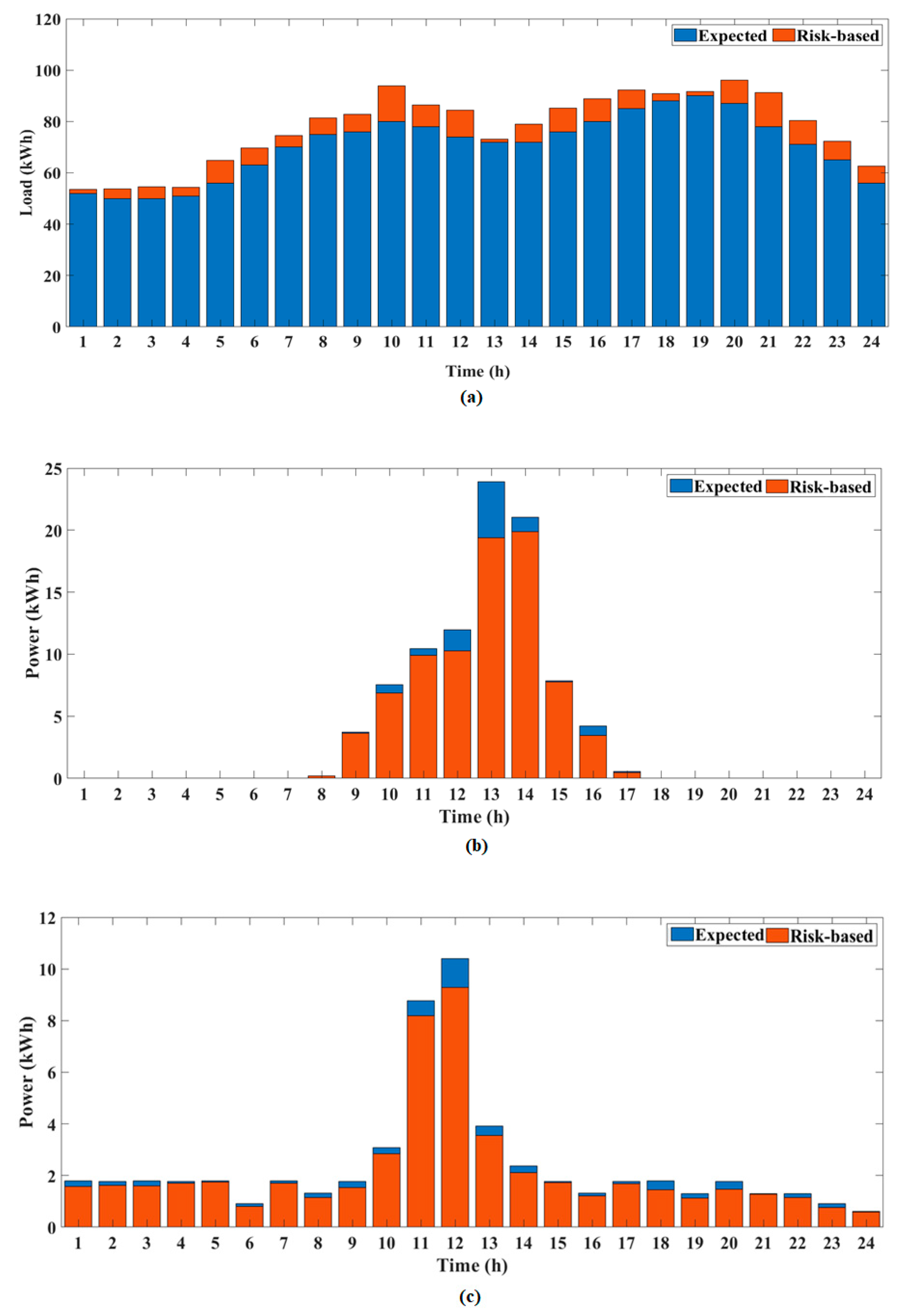
6.2. Proposed Optimization Results

In the first-stage, the MGO uses economic DR among the RH-DRP to optimize MG operation in a day-ahead market with expected scenario. This stage was simulated by considering the hourly average values of load, wind speed, and solar irradiance.

Table 4. Expected wind turbine (WT) and photovoltaic (PV) power.

Hour	PV (kW)	WT (kW)	Hour	PV (kW)	WT (kW)
1	0	1.7850	13	23.9000	3.9150
2	0	1.7850	14	21.0500	2.3700
3	0	1.7850	15	7.8750	1.7850
4	0	1.7850	16	4.2250	1.3050
5	0	1.7850	17	0.5500	1.7850
6	0	0.9150	18	0	1.7850
7	0	1.7850	19	0	1.3020
8	0.2000	1.3050	20	0	1.7850
9	3.7500	1.7850	21	0	1.3005
10	7.5250	3.0900	22	0	1.3005
11	10.4500	8.7750	23	0	0.9150
12	11.9500	10.4100	24	0	0.6150

presents the expected power production of PV and WT for each hour. Here, it is assumed that the MGO must buy all the power produced by the PV/WT at each time of the day. In the second stage, risk costs arising from uncertainty are minimized by the MGO. Figure 6 show the generation scenarios and reduction results using the PDF for each unit. The 4000 scenarios were generated by considering the uncertainty in the MG via Monte Carlo simulations. Subsequently, 20 scenarios were selected via k-means clustering considering the cluster number estimation and simulation times. From the 20 generated scenarios, risk-based operational costs were determined by considering α-CVaR using the RH-DRP.

Figure 7 illustrates the expected and risk-based scenario results of the daily load and power generation capacity of PV and WT. Here, the risk-based scenario is the average value comprising the 10% worst-case scenarios. The daily load increased by 162.69 kW, whereas the total power generated by PV and WT decreased by 9.62 kW and 5.25 kW, compared with the expected scenario, respectively.

Figure 8 shows the optimal results of expected operational costs and CVaR by changing the volume ratio of RH-DRP depending on the degree of risk aversion of MGO. We simulate when the risk aversion parameters are 0.1, 0.5, and 1 to consider various MGOs. MGO with β of 0.1 tends to ignore risk-based scenarios. MGO with β of 0.5 responds appropriately to risk-based scenarios, but do not attempt to avoid them entirely. MGO with β equal to 1 tries to completely avoid risk-based scenarios. When the volume of economic DR increases, the expected costs of MG operation decrease because the MGO can sell surplus power to the utility through load shifting at peak load times. However, risk-based DR capacity is not sufficient to address uncertainty problems; thus, the value of CVaR significantly increases as shown in Figure 8. Meanwhile, the high proportion of risk-based DR increases the expected costs and decreases the CVaR value. In addition, by increasing β, the MGO can decrease CVaR more effectively because they are more risk averse in MG operation.

Figure 9 shows risk-based operational costs depending on risk aversion parameter β (0.1, 0.5, or 1). As shown in Figure 9, when β is 0.1, 0.5, and 1, the optimal solution is that the ratio of economic and risk-based DR is consist of 17.5:2.5, 10:10, and 5:15, respectively. As observed in these results, it should be noted that the MGO who can highly avoid risk should operate within the higher portion of the risk-based DR in RH-DRP.

Table 5. Risk-based optimal operation according to β.

Type	β = 0.1	β = 0.5	β = 1
Expected costs ($)	239.7650	251.9952	255.6907
CVaR ($)	383.1010	86.3655	38.0064
Operational costs ($) (10% worst scenario)	622.8660	338.3607	293.6971

summarizes the results of the risk-based optimal operation in MG. The lowest expected costs are determined when β is 0.1, but CVaR is very high, owing to insufficient management of risk problems. Meanwhile, the expected costs are slightly high when β is equal to 1, but the CVaR is significantly lower than in other cases. In other words, in a 10% worst scenario, in a low-voltage grid-connected MG operation, an MGO would incur operational costs of $622.8660 (β = 0.1), $338.3607 (β = 0.5), or $293.6971 (β = 1). As can be seen from these results, RH-DRP is properly utilized according to the degree of risk aversion of MGO, and it is particularly effective in reducing risk costs for MGO that tend to avoid risk situation caused by uncertainty.

Table 6. Optimal power scheduling (β = 0.1).

Hour	Units (kWh)
	MT	FC	PV	WT	ESS	Utility
1	6.0715	30.0000	0.0000	1.7900	−6.8677	30.0000
2	6.0024	30.0000	0.0000	1.7800	−8.8357	30.0000
3	6.0446	30.0000	0.0000	1.7900	−8.8879	30.0000
4	6.0282	30.0000	0.0000	1.7800	−7.6826	30.0000
5	6.0493	30.0000	0.0000	1.7900	−1.8190	30.0000
6	6.0045	30.0000	0.0000	0.9200	7.3482	30.0000
7	6.0027	30.0000	0.0000	1.7900	14.3143	30.0000
8	6.0005	30.0000	0.2000	1.3100	27.4728	13.7642
9	29.997	30.0000	3.7500	1.7800	30.0000	−29.3026
10	29.0909	30.0000	7.5300	3.0900	30.0000	−30.0000
11	18.7481	30.0000	10.4500	8.7700	30.0000	−30.0000
12	12.1225	30.0000	11.9500	10.4100	30.0000	−30.0000
13	6.0163	30.0000	23.9000	3.9100	28.9134	−30.0000
14	10.3198	30.0000	20.0500	2.3700	30.0000	−30.0000
15	26.5753	30.0000	7.8700	1.7800	30.0000	−30.0000
16	29.9974	30.0000	4.2200	1.3100	30.0000	−25.8165
17	29.9980	30.0000	0.5500	1.7800	30.0000	−17.1583
18	6.0017	30.0000	0.0000	1.7900	30.0000	21.0241
19	6.0002	30.0000	0.0000	1.3000	28.7291	30.0000
20	6.0005	30.0000	0.0000	1.7800	30.0000	17.9934
21	29.9983	30.0000	0.0000	1.3000	30.0000	−23.3302
22	29.9999	30.0000	0.0000	1.3000	30.0000	−15.6415
23	6.0054	30.0000	0.0000	0.9200	4.7649	30.0000
24	6.0074	30.0000	0.0000	0.6200	−2.6961	30.0000

,

Table 7. Optimal power scheduling (β = 0.5).

Hour	Units (kWh)
	MT	FC	PV	WT	ESS	Utility
1	6.0196	30.0000	0.0000	1.7900	−9.6310	30.0000
2	6.0204	30.0000	0.0000	1.7800	−11.8594	30.0000
3	6.0031	30.0000	0.0000	1.7900	−11.8298	30.0000
4	6.2472	30.0000	0.0000	1.7800	−10.9673	30.0000
5	6.0209	30.0000	0.0000	1.7900	−5.1570	30.0000
6	6.0083	30.0000	0.0000	0.9200	3.5573	30.0000
7	6.0050	30.0000	0.0000	1.7900	10.5224	30.0000
8	6.0014	30.0000	0.2000	1.3100	8.9664	30.0000
9	29.9970	30.0000	3.7500	1.7800	30.0000	−25.9567
10	29.9918	30.0000	7.5300	3.0900	30.0000	−27.3799
11	22.1811	30.0000	10.4500	8.7700	30.0000	−30.0000
12	15.3795	30.0000	11.9500	10.4100	30.0000	−30.0000
13	8.0987	30.0000	23.9000	3.9100	30.0000	−30.0000
14	13.4887	30.0000	20.0500	2.3700	30.0000	−30.0000
15	29.9203	30.0000	7.8700	1.7800	30.0000	−30.0000
16	29.9975	30.0000	4.2200	1.3100	30.0000	−22.2957
17	29.9998	30.0000	0.5500	1.7800	30.0000	−14.5210
18	6.0007	30.0000	0.0000	1.7900	30.0000	21.6680
19	6.0001	30.0000	0.0000	1.3000	25.6865	30.0000
20	6.0004	30.0000	0.0000	1.7800	30.0000	19.2081
21	29.9994	30.0000	0.0000	1.3000	30.0000	−19.8983
22	29.9998	30.0000	0.0000	1.3000	30.0000	−18.0410
23	6.0036	30.0000	0.0000	0.9200	2.5509	30.0000
24	6.0600	30.0000	0.0000	0.6200	−4.6747	30.0000

and

Table 8. Optimal power scheduling (β = 1).

Hour	Units (kWh)
	MT	FC	PV	WT	ESS	Utility
1	6.4208	30.0000	0.0000	1.7900	−13.1397	30.0000
2	6.2111	30.0000	0.0000	1.7800	−15.0381	30.0000
3	6.0744	30.0000	0.0000	1.7900	−14.9114	30.0000
4	6.0550	30.0000	0.0000	1.7800	−13.8230	30.0000
5	6.0597	30.0000	0.0000	1.7900	−8.5424	30.0000
6	6.0133	30.0000	0.0000	0.9200	−0.2126	30.0000
7	6.0036	30.0000	0.0000	1.7900	6.3406	30.0000
8	6.0000	30.0000	0.2000	1.3100	30.0000	8.1371
9	29.9989	30.0000	3.7500	1.7800	30.0000	−22.7060
10	29.9963	30.0000	7.5300	3.0900	30.0000	−23.9606
11	25.5194	30.0000	10.4500	8.7700	30.0000	−30.0000
12	18.5466	30.0000	11.9500	10.4100	30.0000	−30.0000
13	11.1802	30.0000	23.9000	3.9100	30.0000	−30.0000
14	16.5702	30.0000	20.0500	2.3700	30.0000	−30.0000
15	29.9993	30.0000	7.8700	1.7800	30.0000	−26.8263
16	29.9983	30.0000	4.2200	1.3100	30.0000	−18.8726
17	29.9990	30.0000	0.5500	1.7800	30.0000	−10.8822
18	6.0004	30.0000	0.0000	1.7900	30.0000	20.9689
19	6.0002	30.0000	0.0000	1.3000	23.4763	30.0000
20	6.0002	30.0000	0.0000	1.7800	30.0000	19.9705
21	29.9992	30.0000	0.0000	1.3000	30.0000	−16.5598
22	29.9989	30.0000	0.0000	1.3000	30.0000	−19.6862
23	6.0179	30.0000	0.0000	0.9200	0.3184	30.0000
24	6.0214	30.0000	0.0000	0.6200	−7.3639	30.0000

present the optimal power scheduling in risk-based MG operation when β is equal to 0.1, 0.5, and 1, respectively. In early periods, the ESS charged and MT output are reduced due to cheap market prices. However, at peak load hours, the battery is fully discharged, and the MGO maximizes local generation to decrease operational costs to sell a considerable amount of energy to the main grid. Owing to low cost of power generation by the FC, the MGO then decides to use its maximum capacity for power supply. Based on the high operational cost of the MT, it is scheduled flexibly while considering the market price. Figure 10 shows RH-DRP participation in MG operation over time. The economic DR is primarily used from 9:00 to 17:00 to reduce the load in common. Through load reduction, the MGO can reduce operational costs by selling remaining power to the main grid when market prices are high. The risk-based DR responds to a power shortage caused by uncertainty and supports MG operation in terms of stability. In MG optimal operation, a larger β value confers a greater risk-based DR portion in RH-DRP. Therefore, it can be confirmed that RH-DRP is efficient for risk-based MG operations considering the risk aversion tendency.

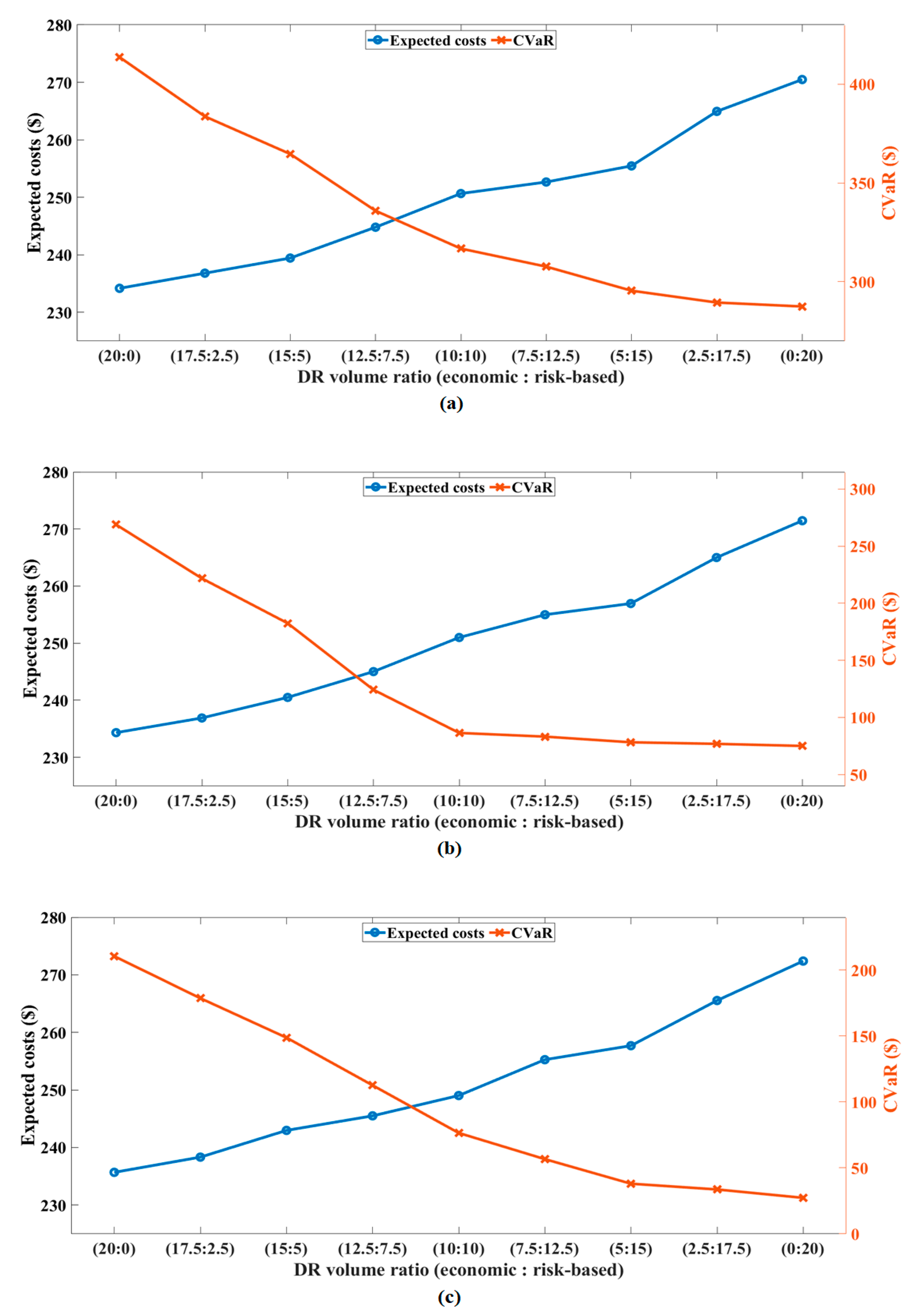
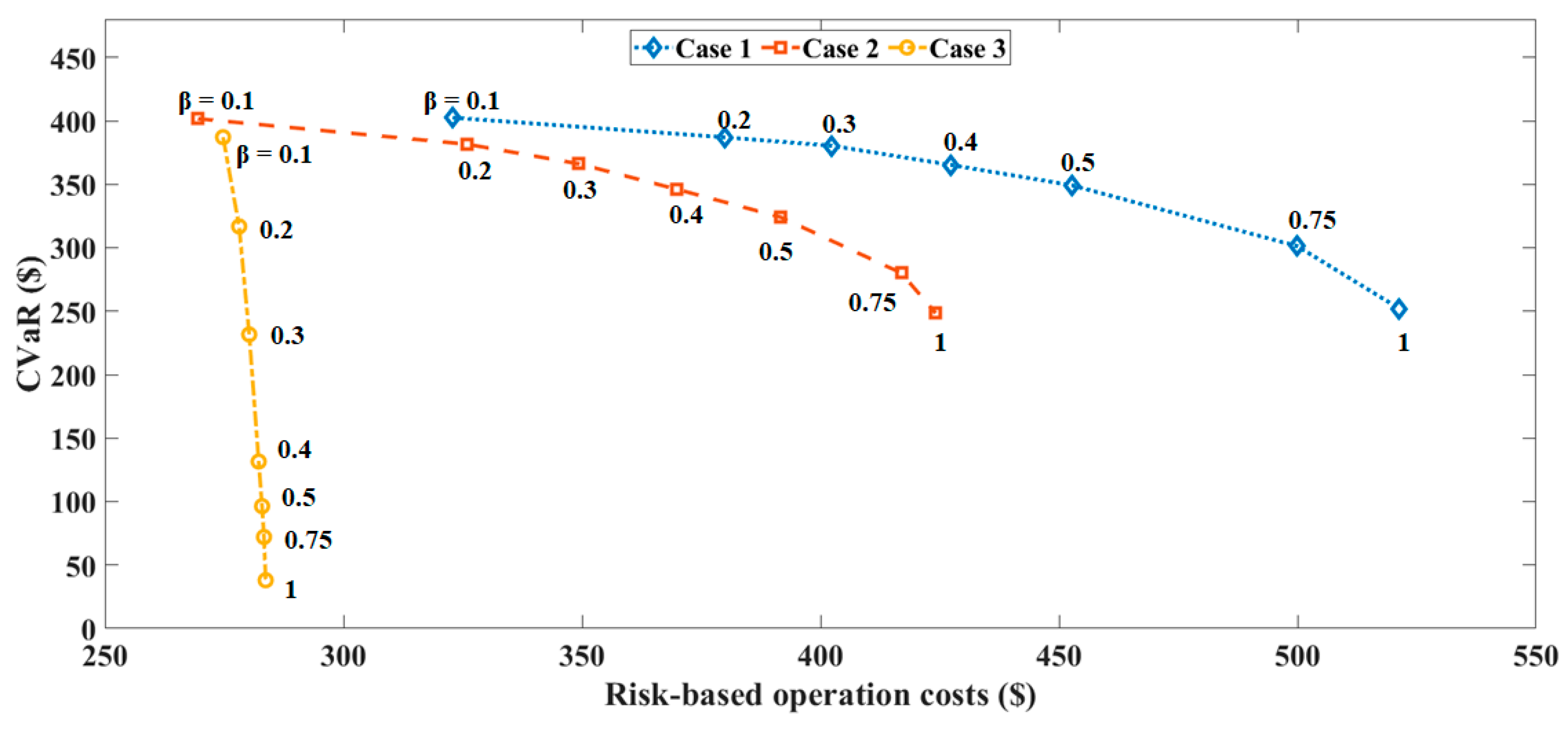
6.3. Comparison of DR Analysis

In the comparison analysis, the effects of RH-DRP are verified by comparing with a different DR strategy for the typical low-voltage MGs operation. To evaluate these strategies, three cases are implemented as follows:

Case 1:

MG operation model without DRP.

Case 2:

MG operation model with prevalent economic DRP.

Case 3:

MG operation model with RH-DRP.

All cases are simulated under the same constraints, but the DRP is different. In Case 1, risk-based costs are determined to purchase only real-time market prices without DRP. Case 2, which considers the prevalent economic DRP, is used to minimize operations costs but does not respond to the risk problem. Case 3 is applied with the proposed DRP strategy, which is the optimal risk-based operation in MG using RH-DRP.

Figure 11 indicates the risk-based operational costs and CVaR at various risk parameter for each case. Case 1 shows high CVaR and risk-based operational costs as peak load reduction and risk control constraints are not considered. As Case 2 utilizes all DRP capacity as economic DR, it shows lower operational costs than Case 1; however, the greater the β value to operate the MG, the higher the risk-based operating costs owing to the lack of risk management capabilities. For Case 3, the CVaR is generally lower that of the other cases because the volume ratio of RH-DRP is appropriately adjusted according to β and risk management is effectively performed; furthermore, owing to proper risk management, the risk-based operational cost does not increase significantly, even when MG is operated with a large value of β. Therefore, when MGOs operate MGs considering uncertainty problems, Case 3 promotes optimal economic and stable operation.

6.4. Performance Test for the IML-ABC

To demonstrate the superiority of IML-ABC, performance tests were evaluated without DRP to fairly compare the IML-ABC with various algorithms.

Table 9. Comparison results for various algorithms.

Algorithm	Best Solution ($)	Worst Solution ($)	Average ($)	Mean Simulation Time (sec)
GA [38]	277.7444	304.5889	290.4321	-
PSO [38]	277.3237	303.3791	288.8761	-
AMPSO [38]	274.4317	274.7318	274.5643	-
θ-PSO [39]	275.3491	281.7841	277.6191	-
GSA [40]	275.5369	282.1743	277.8021	-
ABC	274.3801	274.9271	274.6536	35.28
IML-ABC	272.4761	272.6803	272.5782	29.11

presents optimal results for the forecasted operation costs or each algorithm. The simulation process for different algorithms was repeated 20 times, with the results of the best, worst, and average solutions shown. The IML-ABC algorithm reached an optimal solution compared with the other algorithms. The IML-ABC performs better than the conventional ABC algorithm in terms of simulation time. Figure 12 illustrates the convergence performances of ABC and IML-ABC. The IML-ABC algorithm found the optimal solution during the first iteration, and, when compared with the ABC algorithm, it improved the initial convergence rate. The IML-ABC and ABC reached less than a 0.1% error value compared for the final solution at 168 and 423 iterations, respectively. Therefore, these results verify that the simulation time necessary to find the optimal value is improved by reducing the number of unnecessary iterations.

7. Conclusions

In this study, we proposed two-stage optimal operation of MGs considering uncertainty problems with risk-based DR strategies. To account for uncertainty, WT, PV, and load were modeled as Weibull, Beta, and normal PDF, respectively. The proposed RH-DRP provides a hybrid solution using both economic and risk-based DR to reduce risk-based operational costs. The objective optimization problem consisted of two-stage optimization using the IML-ABC. In the first-stage, the expected operational costs were calculated by deterministic inputs; in the second stage, the risk-based operational costs considered CVaR. To verify the effectiveness of the proposed approach, simulation was conducted on a low-voltage grid-connected MG. The results demonstrate that reasonable operational costs can be determined under the risk aversion parameters compared to conventional optimization solutions. Moreover, our RH-DRP remarkably reduces risk-based operational costs via comparison with various DR strategies. The comparison with various other algorithms also confirmed the superiority of the proposed IML-ABC in identifying the optimal solution and reducing simulation times. Therefore, the proposed approach provides MGOs not only an additional degree of freedom in decision-making under uncertainty but also a solution to reduce risk-based operational costs. Our future work is under way to focus on not only reducing risk-based operating costs but also solving reliability about dynamic problems caused by uncertainty.

References

1. Ding, Z.; Hou, H.; Yu, G.; Hu, E.; Duan, L.; Zhao, J. Performance analysis of a wind-solar hybrid power generation system. Energy Convers. Manag. 2019, 181, 223–234. [Google Scholar] [CrossRef]
2. Millstein, D.; Wiser, R.; Bolinger, M.; Barbose, G. The climate and air-quality benefits of wind and solar power in the United States. Nat. Energy 2017, 2. [Google Scholar] [CrossRef]
3. Jo, K.-H.; Kim, M.-K. Stochastic Unit Commitment Based on Multi-Scenario Tree Method Considering Uncertainty. Energies 2018, 11, 740. [Google Scholar] [CrossRef] [Green Version]
4. Kim, M.K. Multi-objective optimization operation with corrective control actions for meshed AC/DC grids including multi-terminal VSC-HVDC. Int. J. Electr. Power Energy Syst. 2017, 93, 178–193. [Google Scholar] [CrossRef]
5. Mansouri, S.; Ahmarinejad, A.; Ansarian, M.; Javadi, M.; Catalao, J. Stochastic planning and operation of energy hubs considering demand response programs using Benders decomposition approach. Int. J. Electr. Power Energy Syst. 2020, 120, 106030. [Google Scholar] [CrossRef]
6. Kim, H.; Kim, M.-K. Multi-Objective Based Optimal Energy Management of Grid-Connected Microgrid Considering Advanced Demand Response. Energies 2019, 12, 4142. [Google Scholar] [CrossRef] [Green Version]
7. Sharma, S.; Bhattacharjee, S.; Bhattacharya, A. Probabilistic operation cost minimization of Micro-Grid. Energy 2018, 148, 1116–1139. [Google Scholar] [CrossRef]
8. Che, L.; Zhang, X.; Shahidehpour, M.; Alabdulwahab, A.; Abusorrah, A. Optimal interconnection planning of community microgrids with renewable energy y sources. IEEE Trans. Smart Grid 2017, 8, 1054–1063. [Google Scholar] [CrossRef]
9. Alipour, M.; Mohammadi-Ivatloo, B.; Zare, K. Stochastic Scheduling of Renewable and CHP-Based Microgrids. IEEE Trans. Ind. Inform. 2015, 11, 1049–1058. [Google Scholar] [CrossRef]
10. Niknam, T.; Golestaneh, F.; Malekpour, A. Probabilistic model of polymer exchange fuel cell power plants for hydrogen, thermal and electrical energy management. J. Power Sources 2013, 229, 285–298. [Google Scholar] [CrossRef]
11. Motevasel, M.; Seifi, A.R. Expert energy management of a micro-grid considering wind energy uncertainty. Energy Convers. Manag. 2014, 83, 58–72. [Google Scholar] [CrossRef]
12. Wang, M.Q.; Gooi, H.B. Spinning Reserve Estimation in Microgrids. IEEE Trans. Power Syst. 2011, 26, 1164–1174. [Google Scholar] [CrossRef] [Green Version]
13. Rezaei, N.; Kalantar, M. Smart microgrid hierarchical frequency control ancillary service provision based on virtual inertia concept: An integrated demand response and droop controlled distributed generation framework. Energy Convers. Manag. 2015, 92, 287–301. [Google Scholar] [CrossRef]
14. Albadi, M.; El-Saadany, E. A summary of demand response in electricity markets. Electr. Power Syst. Res. 2008, 78, 1989–1996. [Google Scholar] [CrossRef]
15. Aghajani, G.; Shayanfar, H.; Shayeghi, H. Demand side management in a smart micro-grid in the presence of renewable generation and demand response. Energy 2017, 126, 622–637. [Google Scholar] [CrossRef]
16. Jalali, A.; Aldeen, M. Risk-Based Stochastic Allocation of ESS to Ensure Voltage Stability Margin for Distribution Systems. IEEE Trans. Power Syst. 2018, 34, 1264–1277. [Google Scholar] [CrossRef]
17. Kim, S.; Lee, Y.; Kim, M.-K. Flexible risk control strategy based on multi-stage corrective action with energy storage system. Int. J. Electr. Power Energy Syst. 2019, 110, 679–695. [Google Scholar] [CrossRef]
18. Fossati, J.P.; Galarza, A.; Martín-Villate, A.; Fontán, L. A method for optimal sizing energy storage systems for microgrids. Renew. Energy 2015, 77, 539–549. [Google Scholar] [CrossRef]
19. Samadi, P.; Wong, V.W.; Schober, R. Load Scheduling and Power Trading in Systems With High Penetration of Renewable Energy Resources. IEEE Trans. Smart Grid 2016, 7, 1802–1812. [Google Scholar] [CrossRef]
20. Sortomme, E.; El-Sharkawi, M.A. Optimal Power Flow for a System of Microgrids with Controllable Loads and Battery Storage. In Proceedings of the 2009 IEEE/PES Power Systems Conference and Exposition, Seattle, WA, USA, 15–18 March 2009; pp. 1–5. [Google Scholar] [CrossRef]
21. Mohammadi, S.; Soleymani, S.; Mozafari, B. Scenario-based stochastic operation management of MicroGrid including Wind, Photovoltaic, Micro-Turbine, Fuel Cell and Energy Storage Devices. Int. J. Electr. Power Energy Syst. 2014, 54, 525–535. [Google Scholar] [CrossRef]
22. Mazidi, M.; Zakariazadeh, A.; Jadid, S.; Siano, P. Integrated scheduling of renewable generation and demand response programs in a microgrid. Energy Convers. Manag. 2014, 86, 1118–1127. [Google Scholar] [CrossRef]
23. Gazijahani, F.S.; Salehi, J. Optimal Bilevel Model for Stochastic Risk-Based Planning of Microgrids Under Uncertainty. IEEE Trans. Ind. Informatics 2017, 14, 3054–3064. [Google Scholar] [CrossRef]
24. Petrollese, M.; Valverde, L.; Cocco, D.; Cau, G.; Guerra, J. Real-time integration of optimal generation scheduling with MPC for the energy management of a renewable hydrogen-based microgrid. Appl. Energy 2016, 166, 96–106. [Google Scholar] [CrossRef]
25. Kanungo, T.; Mount, D.; Netanyahu, N.; Piatko, C.; Silverman, R.; Wu, A. An efficient k-means clustering algorithm: Analysis and implementation. IEEE Trans. Pattern Anal. Mach. Intell. 2002, 24, 881–892. [Google Scholar] [CrossRef]
26. Shirazi, M.M.H.; Mowla, D. Energy optimization for liquefaction process of natural gas in peak shaving plant. Energy 2010, 35, 2878–2885. [Google Scholar] [CrossRef]
27. Moghaddam, M.P.; Abdollahi, A.; Rashidinejad, M. Flexible demand response programs modeling in competitive electricity markets. Appl. Energy 2011, 88, 3257–3269. [Google Scholar] [CrossRef]
28. Soroudi, A.; Amraee, T. Decision making under uncertainty in energy systems: State of the art. Renew. Sustain. Energy Rev. 2013, 28, 376–384. [Google Scholar] [CrossRef]
29. Khodabakhsh, R.; Sirouspour, S. Optimal Control of Energy Storage in a Microgrid by Minimizing Conditional Value-at-Risk. IEEE Trans. Sustain. Energy 2016, 7, 1264–1273. [Google Scholar] [CrossRef]
30. Karaboga, D.; Basturk, B. A powerful and efficient algorithm for numerical function optimization: Artificial bee colony (ABC) algorithm. J. Glob. Optim. 2007, 39, 459–471. [Google Scholar] [CrossRef]
31. Zhang, H.; Xie, Z.; Lin, H.-C.; Li, S. Power Capacity Optimization in a Photovoltaics-Based Microgrid Using the Improved Artificial Bee Colony Algorithm. Appl. Sci. 2020, 10, 2990. [Google Scholar] [CrossRef]
32. Al-Sakkaf, S.; Kassas, M.; Khalid, M.; Abido, M.A. An Energy Management System for Residential Autonomous DC Microgrid Using Optimized Fuzzy Logic Controller Considering Economic Dispatch. Energies 2019, 12, 1457. [Google Scholar] [CrossRef] [Green Version]
33. Habib, H.U.R.; Subramaniam, U.; Waqar, A.; Farhan, B.S.; Kotb, K.M.; Wang, S. Energy Cost Optimization of Hybrid Renewables Based V2G Microgrid Considering Multi Objective Function by Using Artificial Bee Colony Optimization. IEEE Access 2020, 8, 62076–62093. [Google Scholar] [CrossRef]
34. Aghajani, G.; Shayanfar, H.; Shayeghi, H. Presenting a multi-objective generation scheduling model for pricing demand response rate in micro-grid energy management. Energy Convers. Manag. 2015, 106, 308–321. [Google Scholar] [CrossRef]
35. Faria, P.; Vale, Z. Demand response in electrical energy supply: An optimal real time pricing approach. Energy 2011, 36, 5374–5384. [Google Scholar] [CrossRef] [Green Version]
36. Apx Power Spot Exchange. Available online: https://www.apxgroup.com/trading-clearing/apx-power-uk/ (accessed on 1 December 2019).
37. The Solar Power Group Company. Available online: http://thesolarpowergroup.com (accessed on 1 December 2019).
38. Anvari-Moghaddam, A.; Seifi, A.R.; Niknam, T.; Pahlavani, M.R.A. Multi-objective operation management of a renewable MG (micro-grid) with back-up micro-turbine/fuel cell/battery hybrid power source. Energy 2011, 36, 6490–6507. [Google Scholar] [CrossRef]
39. Baziar, A.; Kavousi-Fard, A. Considering uncertainty in the optimal energy management of renewable micro-grids including storage devices. Renew. Energy 2013, 59, 158–166. [Google Scholar] [CrossRef]
40. Niknam, T.; Golestaneh, F.; Malekpour, A. Probabilistic energy and operation management of a microgrid containing wind/photovoltaic/fuel cell generation and energy storage devices based on point estimate method and self-adaptive gravitational search algorithm. Energy 2012, 43, 427–437. [Google Scholar] [CrossRef]
Figure 1. Schematic representation of two-stage optimal operation.
Energies 13 06052 g001
Figure 2. Determination of α confidence level conditional value at risk (α-CVaR) as a function of power shortages.
Energies 13 06052 g002
Figure 3. Overall process of the proposed optimal operation approach.
Energies 13 06052 g003
Figure 4. Diagram of a low-voltage grid-connected microgrid (MG).
Energies 13 06052 g004
Figure 5. Day-ahead market price of a low-voltage MG.
Energies 13 06052 g005
Figure 6. Scenario generation and reduction results.
Energies 13 06052 g006
Figure 7. Expected and risk-based volumes. (a) Load, (b) photovoltaic (PV) generated, and (c) wind turbine (WT) generated.
Energies 13 06052 g007
Figure 8. Expected operational costs and CVaR for each β. (a) β = 0.1, (b) β = 0.5, and (c) β = 1.
Energies 13 06052 g008
Figure 9. Risk-based operational cost as demand response (DR) volume ratio. (a) β = 0.1, (b) β = 0.5, and (c) β = 1.
Energies 13 06052 g009
Figure 10. Optimal risk-based hybrid demand response program (RH-DRP) participation volume. (a) β = 0.1, (b) β = 0.5, and (c) β = 1.
Energies 13 06052 g010
Figure 11. Optimal solution for each case.
Energies 13 06052 g011
Figure 12. Convergence diagram using both artificial bee colony (ABC) and improved multi-layer (IML)-ABC algorithms.
Energies 13 06052 g012