Abstract
A DC motor velocity control in feedback systems usually requires a velocity sensor, which increases the controller cost. Additionally, the velocity sensor used in industrial applications presents several disadvantages such as maintenance requirements and signal conditioning. In this work, we propose a robust velocity control scheme applied to a DC motor based on estimation strategies using a sliding-mode observer. This means that measurements with mechanical sensors are not required in the controller design. The proposed observer estimates the rotational velocity and load torque of the motor. The controller design applies the exact-linearization technique combined with the super-twisting algorithm to achieve robust performance in the closed-loop system. The controller validation was carried out by experimental tests using a workbench, which is composed of a control and data acquisition Digital Signal Proccessor board, a DC-DC electronic converter, an interface board for signals conditioning, and a DC electric generator connected to an adjustable resistive load. The simulation and experimental results show a significant performance of the proposed control scheme. During tests, the accuracy, robustness, and speed response on the controller were evaluated and the experimental results were compared with a classic proportional-integral controller, which uses a conventional encoder.
1. Introduction
A DC motor is an electromechanical actuator, with the characteristics of being easy to control, having great versatility, and capability for applications with high inertia loads. This makes them suitable in many industrial applications such as steel rolling mills, railway traction, industrial drives, robotics, and precision servos, among others [1,2]. On the other hand, in the feedback DC motor velocity controller, the motor velocity is traditionally measured through the velocity sensor. However, velocity measurement using the velocity sensor tends to increase the controller cost due to it being mechanically assembled with the motor shaft, besides instrumentation is required to signal conditioning [3]. Also, velocity sensors reduce reliability since growth in the number of components increases the possibility of failure. In addition, they decrease noise immunity, due to the physical connection between elements of the acquisition interface board, and sensor wiring. Therefore, the modern trend in motor velocity controller design is the replacement of position sensors, and now applying alternative control techniques without the velocity sensor using estimation techniques [3]. On the other hand, different observers have been proposed for the particular application of battery state of charge, for example in [4], the authors propose a multi-time scale estimator, where, based on the online adapted battery model, the Kalman filter-based state of charge estimator and recursive least squares-based capacity estimator are formulated and integrated in the form of dual estimation. Meanwhile, in [5], a parameterization method combining instrumental variable estimation and bilinear principle is proposed to compensate for the noise-induced biases of model identification. The parameterization method is combined with a Luenberger observer to estimate the state of charge in real-time. Also, in this work, the authors make a comparison of the estimation of the state of charge by using an unscented Kalman filter in three modalities. The results of these estimation methods offer good results.
This paper proposes a robust second-order sliding-mode (SOSM) super-twisting velocity controller applied to a separately excited DC motor. This controller is designed based on input–output feedback linearization control techniques combined with sliding-mode observer. Therefore, the velocity measurement is not required for the controller design. The main idea is to algebraically transform the original system dynamics into an exact linearized system so that the feedback control techniques could be applied. The SOSM controllers are a type of variable structure system in which the state variables of the system are driven over a predetermined trajectory in the state space named sliding surface. When certain conditions are satisfied, the state slides over this surface towards the origin and maintains it there, even in the presence of external disturbances and parameter variations due to temperature changes and the magnetic saturation effect [6]. Consequently, the sliding mode technique is used in many control applications [7,8,9,10,11,12]. The standard sliding-mode generates a high-frequency switching signal that ensures a movement of the sliding variable towards the origin. However, standard sliding-mode produces a chattering effect, which can cause undesirable mechanical vibrations in the controlled system [6]. A method for suppressing the chattering effect is by means of a SOSM technique [13,14]. The SOSM technique generalizes the idea of the standard sliding-modes to restrict movement to the switching surface while maintaining null its first derivative. This controller can be applied to systems where the control input appears in the first derivative of the sliding variable [13,14,15]. A significant SOSM technique for feedback systems is the super-twisting algorithm, which is applied for systems with relative degree one. The controller provides real-time convergence, generates a continuous control signal, and drastically reduces the chattering effect [13]. The literature on SOSM control reports excellent results in several applications [7,9,16,17,18]. It is important to mention that other robust control techniques based on optimization exist. In [19], a distributed control algorithm is proposed to be applied in multi-energy systems where the control law is based on the Lyapunov technique. In [20], an energy management model of multi-energy is proposed for achieving the adaptive change of power generation systems when they change from isolated operation to connected operation with the utility grid. In [21], a distributed control system based on the H-infinity control technique applied to multi-energy systems is proposed. This system solves the uncertainty problem originated by wind and photovoltaic systems, and the load switching. In [22], load aggregation and desegregation models are proposed, applying a strategy algorithm of economic programming with time multi-scales for efficient management. In [23], two level programming is proposed for collaborative management of the distribution of active power in the utility grid to power generation systems for reducing the operation cost of the active power distribution systems and maximizing the profits of each virtual generation power system by considering flexible resources.
This paper shows the controller performance through digital simulations and experimental tests in the laboratory. The validation results exhibit consistent velocity control accuracy, reaching the tracking reference in a fast and smooth way with a precision error in steady-state not greater than 1.0 percent. The maximum current during the transient at start-up is safe for the motor. The velocity observer performance shows consistent accuracy and robustness, and the speed convergence is achieved.
2. DC Motor Model
The DC motor is an electromechanical machine constituted by two main components: a fixed stator, and a rotary part. The stator has a rolled steel core and a set of wire coils named stator field windings. The rotor is constituted by a rolled steel core, rotor coils, and commuter or collector, by which the voltage is supplied. The rotor winding is known as armature winding. All of the armature set is assembled on a steel shaft through which the output mechanical power is developed. Figure 1 shows the equivalent circuit of the DC motor.
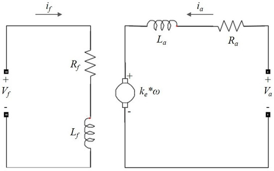
Figure 1.
DC motor equivalent circuit.
The dynamic behavior of this motor is generally described by a set of differential equations, which represent the electrical and mechanical basic phenomena of the motor. It leads to the equilibrium voltage equation in the armature winding and the rotatory motion equation that involve the rotor masses [24]. The accuracy of the model results depends on the detail in which the dynamics of phenomena is described. On the other hand, the DC motor traditionally has been modeled as a system of constant parameters with a linear performance between the electric system and the magnetic field (i.e., the magnetic saturation of the core is not considered). In a separately-excited DC motor, the magnetic field is fed from a constant DC supply and consequently, the field current is constant. Thus, the mathematical model is represented in the state space as follows:
where ia is the current that flows through the armature winding; ωm is the rotor speed and is also the output of the system; km represents the motor constant involved in the electromotive force; Ra and La are the armature winding resistance and inductance, respectively; Jm and Bm are respectively the inertia constant and the viscous friction coefficient of the rotor; TL is a mechanical input known as the load torque; and finally, ua is the control input, which represents the voltage supply for the armature winding.
3. Controller Design
The main goal of the control system is to maintain the motor velocity in preset values. The control consists of a feedback system in which the output variable is compared with a velocity set-point. This comparison represents the deviation of the velocity as controlled variably with respect to the set point. The controller receives the velocity error signal and sends a control action to an actuator so that the error signal is compensated and steered toward a value close to zero.
The velocity control of the DC motor is carried out via the armature voltage supply using the conventional pulse width modulation technique (PWM). Figure 2 shows the proposed velocity scheme, where the motor speed is estimated by the continuous measurement of the armature current ia.
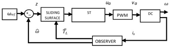
Figure 2.
Control scheme based on armature current measurements.
The control design is based on the exact linearization technique via input–output feedback. This technique focuses basically on differentiating the output function repeatedly until the control input appears explicitly. Subsequently, the control input is designed so that the nonlinearities of the system are canceled, and the system is transformed into an equivalent linear form. Considering a non-linear system single-input single-output (SISO)
Additionally, the repeated differentiation process of the output y in (2) is described in detail in [18]. This process can be represented as follows:
where r is the relative degree of the system and it represents the number of successive differentiations required so that the control input u explicitly appears. The successive differentiations are defined by y(r). The function h(x) denotes the output variable to be differentiated.
If the relative degree is precisely equal to the system order, r = n, then it is said that the system can be transformed to the exact equivalent linear form and the resulting system is known as normal form [24]:
The normal form dynamics expressed as a function of the new variable z, is represented by the equations set as follows:
where z1, z2, …, zn are the state variables, and a(z) and b(z) are the system parameters of the transformed system. Finally, the transformed system combined with the control law changes the original system into an equivalent controllable linear system. The gains of the control law are established by assigning a specific set of eigenvalues in the new system to satisfy a particular performance criterion. In the design process, the motor model (1) is represented in an appropriate form, in which the speed ωm is replaced by x1 and the armature current ia is replaced by x2:
where the tracking error of the controlled output is represented by y = h(x), while x1ref indicates the reference speed set in the controller. Applying differential geometry concepts, the first differentiation of control output is:
Since the control input u is not present in (7), it becomes necessary to differentiate once more. As shown in (8), the system has relative degree two, r = 2. Therefore, the design satisfies the necessary condition for the application of the exact linearization technique, since the relative degree is equal to the order of the system r = n. Thus, the resulting model is a second-order linear system, invariant in time and controllable, taking the following form:
where:
The new system (9) has a relative degree of two, which means that when applying a first-order control law the closed-loop system would not be robust. Then, in order to propose a robust closed-loop system the following system is defined
whose dynamics is:
where:
The new system proposed (12) has a relative degree one, therefore a first-order control law can be applied to establish a robust closed-loop system, such as the super-twisting algorithm of second order sliding modes.
Super-Twisting Control Algorithm
The sliding mode control is a type of variable structure control which acts by applying a discontinuous control input that switches at high frequency and its argument is defined by the system states. The sliding mode control is applied in linear and nonlinear systems.
This sliding mode control provides high precision and robustness in uncertain conditions such as external disturbances and parametric variations [13]. The purpose of the sliding mode control law is to drive the plant output variables over a predetermined trajectory in the state space named sliding surface. The main disadvantage of the first-order sliding mode is the chattering effect that is present in the output variables. However, the super-twisting algorithm of second-order sliding modes adjusts the chattering problem. The super-twisting law is applicable to systems where the control input appears in the time first-derivative of the sliding variable. The control law is composed of two terms, the first is a continuous function of the sliding surface to mitigate the effect of vibration, while the second is defined by the integral of a discontinuous function of the sliding variable. This control law has the following presentation:
where x is the sliding variable. The constants α and λ are controller parameters. UM is the magnitude over which the control u acts in the segment [−UM, UM] in finite time and remains there. Applying the super-twisting algorithm (13) into system (12), the robust closed loop velocity controller takes the following form:
Considering the dynamic system (14), and the positive constants C, KM, Km, UM, q. Sufficient conditions for convergence in finite time are;
where KM and Km are the upper and lower limits of the function ku. Then, with Km > C and λ sufficiently large the controller provides for the appearance in attracting the trajectories in finite time. The control gains λ and α provide finite time attractively of the sliding mode on and , and consequently, an asymptotic movement toward to zero of the velocity tracking error z1 is achieved.
4. Velocity Observer
The first step in the control design is generally to assume that all the state variables are known through measurement. However, it is common that some state variables are not available due to inaccessibility, or their measuring is not economically viable, or to reduce costs. Whereby, some state variables are usually calculated by using an estimation method.
In this work, it is proposed to estimate the DC motor velocity through measurements of the armature current. The velocity estimating is carried out by means of an observer based on the sliding mode control technique.
The proposed observer takes the advantage of the sliding-mode control due to the fact that the sliding mode observer is robust in the presence of noise during the measurement [6]. The sliding mode observer is modeled as follows:
where , and , are the estimated variables that correspond to the velocity, the load torque and the armature current of the motor respectively. The sliding-mode control input applied to the observer model is expressed as follows:
The variable provides for the tracking function of the estimation error, which is the argument on which the super-twisting control will act to make the error estimation converge to zero.
The observation error dynamic is given by:
where the constants l1 and l2 are calculated from the eigenvalues of (18) as follows:
The resulting characteristic polynomial is expressed in the following form:
Comparing (20) with the characteristic polynomial of the desired poles of the observation error dynamics we have:
where l1 and l2 are the calculated parameters which are derived from the assigned eigenvalues, and that guarantee the stable operation of the observer. Table 1 shows the super-twisting controller parameters.

Table 1.
Observer parameters.
5. Control Scheme Validation
Digital simulations and experimental tests were carried out to validate the velocity controller. Figure 3 shows the control scheme proposed.
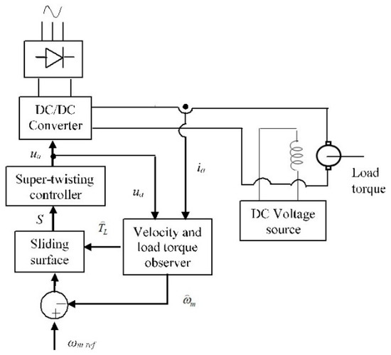
Figure 3.
Configuration scheme of experimental tests.
Simulations were programming in Simulink/Matlab software using the model parameters of the DC motor whose rated values are 0.175 kW, 120 V, 1800 rpm. The electric DC motor parameters are described in Table 2.
Table 2.
DC motor parameters.
5.1. Simulation Results
The DC motor velocity controller performance was evaluated by mean of three disturbances on the load torque and three values for speed reference. The main purpose of the validation tests was to verify robustness, accuracy, and response speed of the controller during the tracking of the reference velocity and the load torque variations. Besides, it also verified the performance of the velocity and load torque observer, considering nonzero initial condition. Additionally, the maximum value of the starting current is limited. Furthermore, an experimental test was configured to compare the controller performance against the performance of a traditional PI controller based on velocity measurements through a conventional encoder. The velocity controller performance during changes on both reference tracking and load torque is shown in Figure 4. The motor is subject initially to a zero speed reference, as shown in Figure 4a. Next, we have a speed reference change from 0 to 60 rad/s and then from 60 to 100 rad/s. Subsequently, a rectangular wave patter is applied with a range of 100 to 140 rad/s. Note that the super-twisting controller action allows a smooth steady-state condition in the transient response of motor velocity to be achieved. The velocity stabilization time is not greater than 0.5 s. The accuracy error of the control variable during velocity changes is lower than one percent.
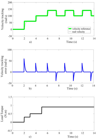
Figure 4.
(a) velocity reference tracking, (b) velocity error tracking, (c) load torque.
An increase in the load torque from 0.3 Nm to 0.5 Nm is applied when time reaches three seconds and other increases are considered from 0.5 Nm to 0.9 Nm when time reaches five seconds, as shown in Figure 4c. During the changes in load torque, the velocity as controlled output stabilizes in no more than 10 ms, with an accuracy error lower than one percent. The steady-state operation takes place when the electromagnetic torque of the motor is equal to the applied load torque. The dynamic behavior of the tracking error variable set in (z1) is shown in Figure 4b, with a peak value of 60 rad/s during the velocity transient response. Figure 4 shows that the assessment of velocity error is close to zero due to its dependency on the velocity observer (16). On the other hand, the voltage as control input and armature current of the motor is shown in Figure 5. The control input acts to steer the speed error towards the origin and maintains it there, even in the presence of external disturbances and parameter variations, as shown in Figure 5a. The armature current suddenly changes to achieve steady-state following the requirements imposed by changes in both velocity reference and load torque, as displayed in Figure 5b. The motor starting current reaches a transient peak no more than 8 A.
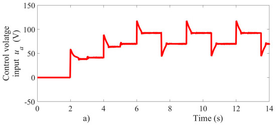
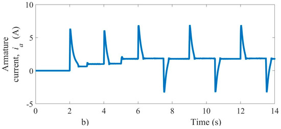
Figure 5.
(a) voltage control input, (b) armature current.
The simulation results of the proposed controller show that the motor current is limited during the transient stage (when the reference velocity changes from 0 to 60 rad/s) by the action of the super-twisting controller. The maximum current allowed is safe for the motor, and the voltage drop across the power supply must be within acceptable limits, too. Test results show that the action of the controller helps to reduce the peak current at startup significantly. The performance of the velocity and load torque observer is shown in Figure 6.
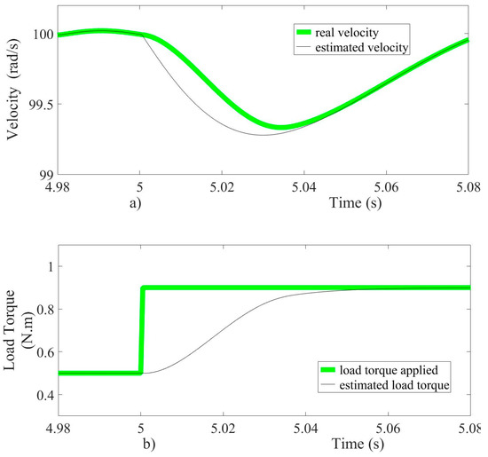
Figure 6.
(a)Velocity and (b) load torque estimation performance.
As can be seen in Figure 6a,b, the velocity and load torque observer prove to be fast converging and accurate. The velocity observer estimates the velocity based on the armature current measurement, and the estimated velocity is then introduced in the control scheme. The velocity and load torque estimation errors are quickly steered to zero, as shown in Figure 7a,b. The results show that the observer performance is satisfactory, ensuring robustness and fast response.
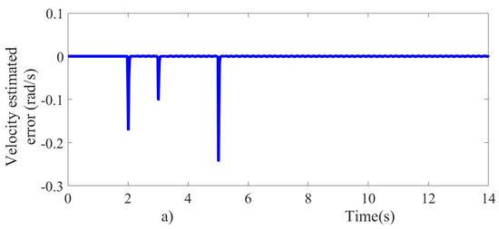
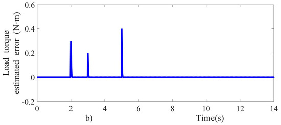
Figure 7.
Estimated tracking errors; (a) velocity and (b) load torque.
5.2. Experimental Results
The proposed velocity controller and the sliding mode observer were validated through experimental tests into laboratory. A DC/DC electronic converter supplied to a 0.175 kW DC motor, whose rated values are shown in Table 2. The motor was coupled via a belt with a DC electric generator that fed to an adjustable resistive load. Variations in motor load torque were established by varying the resistive load. The data acquisition and control algorithm were processed in a DS1104 Controller Board using a sampling frequency of 100 kHz. The armature current was measured by means of a fully-differential isolation amplifier. The proposed velocity controller that uses the armature current to estimate the velocity was experimentally compared with a PI controller that uses an incremental optical encoder. The Simulink tool Real-Time Workshop was used to implement a base program with the input and output conditioning interfaces.
Figure 8 shows the hardware that was used for the DC motor velocity controller tests. In the laboratory tests, velocity regulation was maintained while diverse changes in load torque were made to the load resistance of a DC generator. The velocity error variable is defined with the difference between the velocity reference and the velocity estimated by the observer. The sliding surface was established with the velocity error variable and its time first derivative. The sliding surface is the argument of the super-twisting control algorithm, which generates a continuous control signal which is conditioned to supply voltage to the motor.
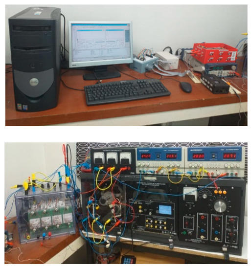
Figure 8.
Hardware for the DC motor velocity controller.
The velocity controller performance during experimental tests is shown in Figure 9. Changes simultaneous in the velocity reference and load torque are applied. The motor was initially subject to a zero speed reference; afterward, the velocity reference changed from 0 to 120 rad/s, as shown in Figure 9a. Subsequently, a periodic square function (pulse train) was configured that varies from 120 to 150 rad/s with a period of 4 s. The super-twisting control algorithm forces the sliding surface toward zero; and consequently, an asymptotic movement of the velocity is achieved. The stabilization time of the velocity is lower than one second, such as shown in Figure 9a. The dynamic behavior of the velocity tracking error is shown in Figure 9b.
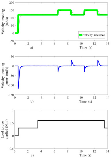
Figure 9.
Experimental test results, (a) velocity reference tracking, (b) velocity error tracking, (c) load torque applied.
The relative velocity error in steady state is not greater than 0.2 percent, with a peak value of −120 rad/s during the startup. Therefore, the velocity error in steady state is very close to zero, as is shown in Figure 9b. A second increase in the load torque from 0.3 Nm to 0.6 Nm is applied in 3.5 s, as shown in Figure 9c. The changes of the load torque considered as external disturbances are rejected by the super-twisting control algorithm, and then the velocity tracking is achieved in smooth form. Meanwhile, the voltage as control input and the motor armature current are shown in Figure 10. The control input acts to steer the velocity error variable towards zero asymptotically.
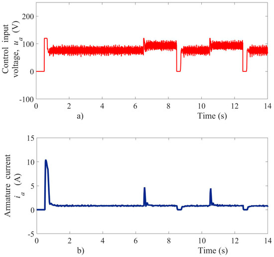
Figure 10.
Experimental test results, (a) voltage control input, (b) armature current.
The armature current suddenly changed due to sudden variations of the load torque and velocity reference, as shown in Figure 10b. The input voltage signal presented an oscillation frequency around 5 kHz within a voltage oscillation-band of magnitude 20.5 V in steady-state conditions. The armature current in the startup achieved a peak near 10 A, as shown in Figure 10b. This current did not affect the motor operation, and the voltage drop in power supply source caused by the motor starting also was within acceptable limits. On the other hand, the sliding mode observer proved fast convergence and accuracy even with a different initial condition, as shown in Figure 11a. The velocity estimation errors were quickly steered to zero, as shown in Figure 11b. In order to validate the velocity observer performance, an initial condition of 38 rad/s was set in the estimated velocity when the first velocity reference appears, and the velocity observer shows a fast convergence of 200 ms, approximately.
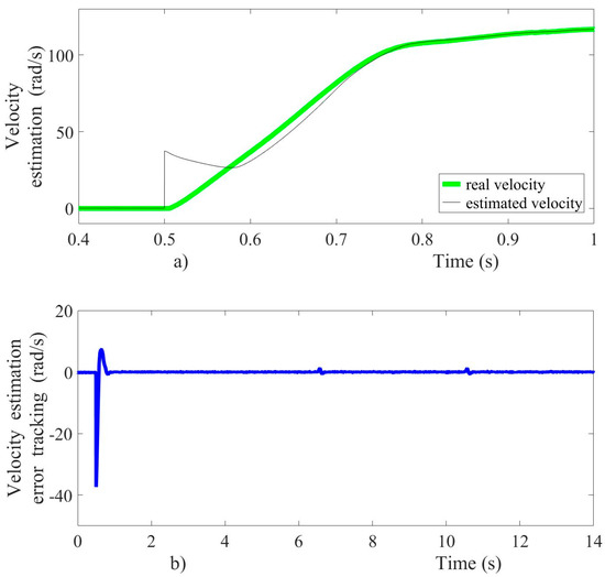
Figure 11.
Velocity observer performance; (a) velocity estimation, (b) velocity error estimation.
Figure 12 shows a comparison between the velocity controller using the super-twisting algorithm without encoder and the velocity controller using PI algorithm with a conventional encoder. Both controllers operated under the same load torque changes and with the same velocity reference.
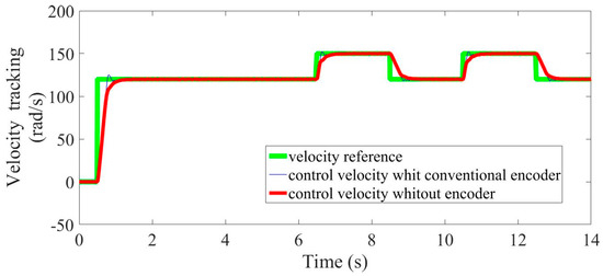
Figure 12.
Comparison of experimental results of velocity trajectories tracking.
Both controllers show satisfactory results, particularly in the steady-state region. However, in the transient zone, the super-twisting controller offered greater precision and robustness compared with the PI controller. Besides, the super-twisting controller had a significantly faster settling time and reached the steady-state in a smooth form, meanwhile the PI controller had an overshoot of 2 percent, approximately. This behavior can also been seen in Figure 13 by means of the velocity tracking error.
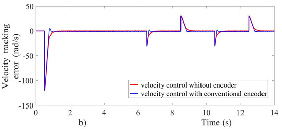
Figure 13.
Velocity error tracking during experimental tests.
6. Conclusions
In this paper, a robust velocity controller without mechanical sensor applied to a separately excited DC motor was proposed. The control strategy is based on the armature current measurement and the application of a robust control law of second-order sliding-mode called the super-twisting algorithm. A sliding-mode observer allows estimating the angular velocity and the load torque of the motor, in a fast and precise form. The DC motor velocity controller has a robust performance in the presence of uncertain conditions, such as changes in the load torque and in the velocity reference. In addition, regardless of robust performance, the proposed controller has a lower cost compared with a controller using a conventional encoder. Consequently, the proposed controller can be useful in many industrial applications at a lower cost. Then, as future work, the proposed method will extend to induction motor velocity control. However, a limitation of the proposed control is that the current and voltage sensors should be sufficiently accurate for a good variable estimation.
Author Contributions
Conceptualization, R.R. and F.A.V.; Formal analysis, C.E.C.; Investigation, R.R. and O.A.M.; Methodology, F.A.V., F.M. and O.A.M.; Resources, F.M.; Software, F.M. and C.E.C.; Writing—original draft, R.R. and F.A.V. All authors have read and agreed to the published version of the manuscript.
Funding
This research received no external funding.
Conflicts of Interest
The authors declare no conflict of interest.
References
- Hughes, A.; Drury, B. Electric Motors and Drives Fundamentals, Types and Applications, 5th ed.; Elsevier Ltd.: Amsterdam, The Netherlands, 2019. [Google Scholar] [CrossRef]
- Anatoli, S.; Naung, Y.; Lin, H.O.; Khaing, Z.M.; Zaw, K.Y. The comparative analysis of modelling of simscape physical plant system design and armature-controlled system design of DC motor. In Proceedings of the 2017 IEEE Conference of Russian Young Researchers in Electrical and Electronic Engineering (EIConRus), St. Petersburg, Russia, 1–3 February 2017; pp. 998–1002. [Google Scholar] [CrossRef]
- Ramírez, R.; Valenzuela, F.A.; Martínez, F.; Castañeda, C.E.; Morfin, O.A.; Olmos, J.A. Speed control of a DC motor based on armature current measurement. Ing. Investig. y Tecnol. 2018, 19. [Google Scholar] [CrossRef]
- Wei, Z.; Zhao, J.; Ji, D.; Tseng, K.J. A multi-timescale estimator for battery state of charge and capacity dual estimation based on an online identified model. Appl. Energy 2017, 204, 1264–1274. [Google Scholar] [CrossRef]
- Wei, Z.; Dong, G.; Zhang, X.; Pou, J.; Quan, Z.; He, H. Noise-immune model identification and state of charge estimation for lithium-ion battery using bilinear parameterization. IEEE Trans. Ind. Electron. 2020. [Google Scholar] [CrossRef]
- Utkin, V.; Guldner, J.; Shi, J. Sliding Mode Control in Electro-Mechanical Systems; CRC Press, Taylor & Francis Group: New York, NY, USA, 2009. [Google Scholar] [CrossRef]
- Tang, Y.; Zhang, Y.; Hasankhani, A.; Zwieten, J.V. Adaptive Super-Twisting Sliding Mode Control for Ocean Current Turbine-Driven Permanent Magnet Synchronous Generator. In Proceedings of the 2020 American Control Conference (ACC), Denver, CO, USA, 1–3 July 2020; pp. 211–217. [Google Scholar] [CrossRef]
- Ferrara, A.; Incremona, G.P.; Sangiovanni, B. Tracking control via switched Integral Sliding Mode with application to robot manipulators. Control Eng. Pract. 2019, 90, 257–266. [Google Scholar] [CrossRef]
- Yousri, M.S.; Derbeli, M.; Barambones, O.; Cheknane, A. Design and Implementation of High Order Sliding Mode Control for PEMFC Power System. Energies 2020, 13, 4317. [Google Scholar] [CrossRef]
- Ruderman, M.; Fridman, L.; Pasolli, P. Virtual sensing of load forces in hydraulic actuators using second- and higher-order sliding modes. Control Eng. Pract. 2019, 92, 104151. [Google Scholar] [CrossRef]
- Fridman, L.; Levant, A. Higher Order Sliding Modes. In Sliding Mode Control in Engineering; Barbot, J.P., Perruguetti, W., Eds.; Marcel Dekker: New York, NY, USA, 2002. [Google Scholar]
- Levant, A. Principles of 2-sliding mode design. Automatica 2007, 43, 576–586. [Google Scholar] [CrossRef]
- Bartolini, G.; Fridman, L.; Pisano, A.; Usai, E. Modern Sliding Mode Control Theory: New Perspectives and Applications; Springer Science: New York, NY, USA, 2008; Volume 375. [Google Scholar]
- Ahmed, Q.; Bhatti, A.I.; Iqbal, S.; Kazmi, I.H. 2-sliding mode based robust control for 2-DOF helicopter. In Proceedings of the 2010 11th International Workshop on Variable Structure Systems (VSS), Mexico City, Mexico, 26–28 June 2010; pp. 481–486. [Google Scholar] [CrossRef]
- Bartolini, G.; Pisano, A.; Punta, E.; Usai, E. A Survey of Applications of Second-order Sliding Mode Control to Mechanical Systems. Int. J. Control 2003, 76, 875–892. [Google Scholar] [CrossRef]
- Davila, J.; Fridman, L.; Levant, A. Second-order sliding-mode observer for mechanical systems. IEEE Trans. Autom. Control 2005, 50, 1785–1789. [Google Scholar] [CrossRef]
- Krause, P.C.; Wasynczuk, O.; Sudhoff, S.D. Analysis of Electric Machinery and Drive Systems; IEEE Press: Piscataway, NJ, USA, 2002. [Google Scholar]
- Isidori, A. Nonlinear Control Systems; Springer: New York, NY, USA, 1995. [Google Scholar]
- Li, Y.; Zhang, H.; Liang, X.; Huang, B. Event-Triggered-Based Distributed Cooperative Energy Management for Multienergy Systems. IEEE Trans. Ind. Inform. 2018, 15, 2008–2022. [Google Scholar] [CrossRef]
- Li, Y.; Gao, D.W.; Gao, W.; Zhang, H.; Zhou, J. Double-Mode Energy Management for Multi-Energy System via Distributed Dynamic Event-Triggered Newton-Raphson Algorithm. IEEE Trans. Smart Grid 2020, 11, 5339–5356. [Google Scholar] [CrossRef]
- Zhou, J.; Xu, Y.; Sun, H.; Wang, L.; Chow, M.Y. Distributed Event-Triggered H∞ Consensus Based Current Sharing Control of DC Microgrids Considering Uncertainties. IEEE Trans. Ind. Inform. 2020, 16, 7413–7425. [Google Scholar] [CrossRef]
- Yi, Z.; Xu, Y.; Gu, W.; Wu, W. A Multi-Time-Scale Economic Scheduling Strategy for Virtual Power Plant Based on Deferrable Loads Aggregation and Disaggregation. IEEE Trans. Sustain. Energy 2020, 11, 1332–1346. [Google Scholar] [CrossRef]
- Yi, Z.; Xu, Y.; Zhou, J.; Wu, W.; Sun, H. Bi-Level Programming for Optimal Operation of an Active Distribution Network With Multiple Virtual Power Plants. IEEE Trans. Sustain. Energy 2020, 11, 2855–2869. [Google Scholar] [CrossRef]
- Khalil, H.K. Nonlinear Systems, 3rd ed.; Pearson Education: New York, NY, USA, 2002. [Google Scholar]


Publisher’s Note: MDPI stays neutral with regard to jurisdictional claims in published maps and institutional affiliations. |
© 2020 by the authors. Licensee MDPI, Basel, Switzerland. This article is an open access article distributed under the terms and conditions of the Creative Commons Attribution (CC BY) license (http://creativecommons.org/licenses/by/4.0/).