Experimental Long-Term Investigation of Model Predictive Heat Pump Control in Residential Buildings with Photovoltaic Power Generation

Abstract

This article presents a 125-day experiment to investigate model predictive heat pump control. The experiment was performed in two parallel operated systems with identical components during the heating season. One of the systems was operated by a standard controller and thus represented a reference to evaluate the model predictive control. Both test rigs were heated by an air-source heat pump which is influenced by real weather conditions. A single-family house model depending on weather measurement data ensured a realistic heat consumption in the test rigs. The adapted model predictive control algorithm aimed to minimize the operational costs of the heat pump. The evaluation of the measurement results showed that the electrical energy demand of the heat pump can be reduced and the coefficient of performance can be increased by applying the model predictive controller. Furthermore, the self-consumption of photovoltaic electricity, which is calculated by means of a photovoltaic model and global radiation measurement data, was more than doubled. Consequently, the energy costs of heat pump operation were reduced by 9.0% in comparison to the reference and assuming German energy prices. The results were further compared to the scientific literature and short-term measurements were performed with the same experimental setup. The dependence of the measurement results on the weather conditions and the weather forecasting quality are shown. It was found that the duration of experiments should be as long as possible for a comprehensive evaluation of the model predictive control potential.

1. Introduction

In developed countries, residential and commercial buildings cause up to 40% of the total final energy consumption. Heating, ventilation, and cooling (HVAC) energy consumption is showing particular growth [1]. In order to counteract this development and to reduce the environmental impact of HVAC systems, efficient control methods are necessary [2]. The impact of control systems on energy consumption due to HVAC systems is explored in various scientific publications. For example, Salvadori et al. [3] recently investigated the energy savings that can be achieved by different control concepts of the heating system in the case of an office building. Within the context of promising control methods, model predictive control (MPC) is of particular interest, as it is able to consider multiple objectives [2,4]. The high energy saving potential of MPC in comparison to common control methods has already been shown in various simulation studies. In particular, Oldewurtel et al. [5] presented a comprehensive system variation.

Next to the control of conventional heating systems, MPC is a suitable method for controlling electric heat pumps [6]. Heat pumps currently show significantly increasing heating system market shares, as the environmental impact of heat pumps in operation is low [7]. Simulation studies of single-family house heat pump systems proved that energy costs can be reduced by the application of MPC [8,9]. Kajgaard et al. [8] indicated the potential of energy cost reduction of up to 12% while Halvgaard et al. [9] stated a 35% reduction potential for heat pump load shifting and varying electricity prices. A publication by Bechtel et al. [10] revealed cost savings of up to 24.3% for single family houses in Luxembourg depending on the heat storage size, when variable electricity prices based on the electricity market are applied. Further studies verify the economic and energetic viability of MPC application for cooling purposes [11] or if the heat pump is combined with a micro heat and power system [12], a fuel cell [13], or solar heat generation [14]. However, heat pumps are assumed to be primarily combined with photovoltaics (PV) in future residential energy systems [15], as the generated electric energy can be directly converted into useful heat avoiding grid feed-in. In this context, experiments were conducted by Franco and Fantozzi [16] in order to analyze the operating performance of the integration of PV and ground source heat pump for a residential building.

As stated by Salpakari and Lund [17], the application of MPC is beneficial for combined heat pump and PV systems, as the amount of PV electricity feed-in is reduced by up to 88%. The self-consumption of PV electricity can be profitable in case of electricity prices which extend electricity grid feed-in remuneration. The authors [17] achieved a 25% energy cost reduction in the case of flexible market electricity prices of Finland and in comparison to a rule-based controller. Furthermore, CO₂-emissions and feed-in peaks could be reduced [18]. In a similar study, Fischer et al. [19] achieved cost savings of 6% to 11% for constant electricity prices and up to 16% for variable electricity prices in comparison to a common rule-based controller. Rastegarpour et al. [20] investigated different MPC approaches for modulating air-to-water heat pumps in radiant-floor buildings. For the considered application, nonlinear MPC has the potential to save up to 6% energy and improve the comfort by 4% with respect to standard MPC. For MPC online optimization, calculation speed and reliability are crucial parameters. In this regard, Gelleschus et al. [21] performed a one-year simulation for a home energy system consisting of a heat pump, a thermal storage, a photovoltaic system, and a battery and compared different algorithms for solving the underlying optimization problem. In a further study [22], a multi-objective home energy management concept using stochastic mixed-integer linear programming and MPC was presented for a grid-coupled home energy system with a PV plant, a battery, and a combined heat pump/heat storage device for domestic hot water supply. It is shown that this concept reduces energy costs as well as the maximum grid loads both on feed-in and demand sides. Hence, it offers a potential for infrastructure cost reduction, if adopted by a large number of prosumers and can lead to a positive effect on the lifetime of the battery.

In contrast to theoretical studies, experimental studies are currently only available in limited numbers. However, experiments should be carried out for a more detailed understanding and potential assessment [6]. Furthermore, experimental studies mostly focus on public buildings [23,24], partly with comparison of the measurement results to a reference case simulation [25]. For the reliability of investigations on the application of MPC in residential buildings, test results should be evaluated by reference experiments. For this purpose, however, two identical residential buildings or suitable test facilities are necessary. Frison et al. [26] presented such a test facility, including a ground-source heat pump. In a first test of a single day, 3.1% of the energy costs could be saved by applying the MPC. Another suitable system for air-source heat pumps was presented by Péan et al. [27]. In a three-day test, which could be repeated with a rule-based controller in the identical plant due to the application of a climate chamber, the MPC could save 7% of the energy costs. However, both authors did not consider PV energy production and the optimization of self-consumption by MPC. This was investigated in short-term measurements by Kuboth et al. [28]. An MPC control algorithm was developed, applied to an air-source heat pump test facility and evaluated. The reference for evaluation was given by a test rig with identical components and common PI-control. Both heat pumps were affected by real weather conditions. In a series of 6 measurements of 120 h each, the MPC algorithm could increase the heat pump coefficient of performance (COP) by a weighted average of 22.2% and the PV self-consumption rate by 234.8%, while the energy costs were reduced by an average value of 34.0% assuming German energy prices.

Overall, it appears that investigations of long-term behavior using an MPC in heat pump control for domestic buildings have been solely performed in theoretical studies based on simulation models. Published experimental studies cover an observation period of a maximum of three days.

Thus, within this article, the promising results deriving from simulations and short-term experiments are to be further evaluated by a long-term measurement applying the identical two test rigs of the short-term measurements. The long-term measurement was carried out in the heating season of the following year over a period of 125 days. Both the short-term and long-term comparison as well as the test duration represent novelties in the experimental investigation of heat pump MPC of detached houses.

2. Experimental Setup

In order to compare a heat pump system with standard control to a model predictive controlled one, a test rig consisting of two identical heat pump devices has been developed. The overall setup as well as its components are described in Section 2.1. Information about the standard control that is applied for the reference test rig are given in Section 2.2.

2.1. Test Rig Setup

The experimental setup for the investigation of model predictive heat pump control comprised two test rigs with identical components. One of the test rigs was operated applying a standard control method (presented in Section 2.2) and served as a reference for the MPC plant. The setup of each test rig is shown in Figure 1.

The air-source heat pumps of the test rigs were placed outside of the laboratory. Therefore, they were influenced by real weather conditions occurring at their location at the University of Bayreuth in Bayreuth Germany. The heat pumps of the type WPL AR 6, manufactured by Bosch Thermotechnik (Kulmbach, Germany) [29], had a nominal thermal power of 6 kW at a flow temperature of 35 °C and an outside air temperature of 2 °C. Generated heat was stored in a water storage with a volume of 500 L before being dissipated by means of a separate water cycle, a heat exchanger, and a cooling water cycle with a flow temperature of 16 °C. Three-way mixing valves included into the cooling water cycles enabled control of the thermal output power.

The thermal power to be dissipated was calculated by two identical building models, one for each test rig. The single-family building models according to Dott et al. [30] had a floor area of 140 m² and a nominal annual heat demand of 45 kWh/m² for the reference weather of Strasbourg. Within the test rig, the heat demand was dynamically specified by the building model and heating system control. Thermal losses and gains were calculated by means of a thermal resistance and capacity network as well as the measured ambient air temperature and solar irradiation. Consequently, the thermal capacity of the floor heating systems was taken into account. Therefore, cooling within the test rigs corresponded to the heat demand of real floor heating systems. Conversely, the floor heating systems were heated by the heat output, which could be calculated by means of the temperature and volume flow measurements, thus ensuring energy conservation. The models were discretized by the explicit Euler method with a time step size of 1 s.

In addition to the building model, a south-facing PV system with a peak power of 4.8 kW and an installation angle of 45° was represented by real-time simulation. Radiation on the inclined surface was determined by the measured horizontal radiation and the calculated date- and time-dependent relative sun-angle. Subsequently, a single diode equivalent circuit model developed by de Soto et al. [31] was linked to the measured values of the solar irradiation and the outside temperature for PV system power calculation. Global horizontal radiation measurement was performed by a thermopile pyranometer of secondary standard accuracy. The share of PV electricity self-consumption was determined considering identical electric load profiles of the building electronics [25] and the measured electric energy consumption of the heat pumps. Self-consumption priority was given to the electric load of the buildings, which consume 3962 kWh of electric energy per year.

The COP was calculated using the following:

$$\mathrm{COP}=\frac{\dot{Q_{\mathrm{HP}}}}{P_{\mathrm{comp}}+P_{\mathrm{pump}}+ P_{\mathrm{fan}}}$$

(1)

where the electric power of the fan P_fan, the electric power of the heat pump compressor P_comp as well as the power of the circulation pump P_pump belonging to the heat pump had to be monitored. In case of the reference test rig, separate current and voltage measurements were performed with accuracies of 0.25% of the measurement range (MR), respectively, in order to determine the electric power. The required current transformer added a further inaccuracy of 0.2% of MR to the current measurement. To ensure a reliable evaluation of the MPC concept, power metering of the MPC test rig heat pump is more accurate. The measurement meters determined the power with an accuracy of 0.2% of the measurement value and additional 0.1% of MR, while digital signals were transferred without additional errors. The heat pump heat flow rate ${\dot{Q}}_{\mathrm{HP}}$ was calculated by an energy balance. Domestic heat pumps were generally operated with high water mass flow rates and a low temperature difference of the flow and return temperature in order to achieve a high COP. Due to the low temperature difference, sensors with high accuracy were necessary to determine energy balances with sufficient accuracy. Therefore, temperatures were measured by calibrated platinum resistance thermometers with a measurement uncertainty of ± (0.1 °C + 0.167% ∙ |ϑ|). Volume flow rates were determined by magnetic-inductive flow meters with an uncertainty of ±0.5% of the measured value.

Total measurement uncertainties were obtained by means of the square-root rule published by Taylor [32]. As the uncertainties in electric power measurements are significantly lower than the uncertainties in determination of thermal power (due to the low temperature differences), the resulting uncertainties in COP approximately corresponded to those of thermal power. For a typical operating point, uncertainties of around 7% occur. The comparability of the test rigs have been proofed in a reference test of 120 h without application of MPC [28].

2.2. Reference Test Rig Control

The control valve regulates the building zone temperature analogous to a real heating system valve. The set building zone temperature of the reference system was 21 °C. Within this system, the control valve and the mixing valve were PI-controlled. Details on the controller settings are given in a previous publication [28].

The outdoor air temperature ϑ_a represents a reference value for controlling the heat generation of the reference test rig heat pump. The set flow temperature of the heat pump

$${\vartheta }_{\mathrm{f}}=\left({\vartheta }_{\mathrm{f},\mathrm{nom}}–{\vartheta }_{\mathrm{z},\mathrm{nom}}\right){\left(\frac{{\vartheta }_{\mathrm{z},\mathrm{nom}} – {\vartheta }_{\mathrm{amb}} }{{\vartheta }_{\mathrm{a},\mathrm{nom}} – {\vartheta }_{\mathrm{amb},\mathrm{nom}}}\right)}^{\frac{1}{n}}+ {\vartheta }_{\mathrm{z},\mathrm{nom}}$$

(2)

can be calculated by a heating curve function, where the exponent n is set to 1.1 relating to floor heating systems. The nominal set flow temperature ϑ_f,nom at a nominal ambient temperature ϑ_a,nom of −20 °C was set to 38 °C. As this value was determined to be the lowest possible set temperature to keep the occupants’ thermal comfort, flow temperature was kept as low as possible and the resulting heat pump COP was maximized for the applied control type in the reference test rig. The nominal zone temperature ϑ_z,nom was 20 °C. The flow temperature of the heat pump was measured at the top of the heat storage. Another controller regulated the heat pump heat generation in order to adapt the measured flow temperature to the desired set point.

3. Model Predictive Control

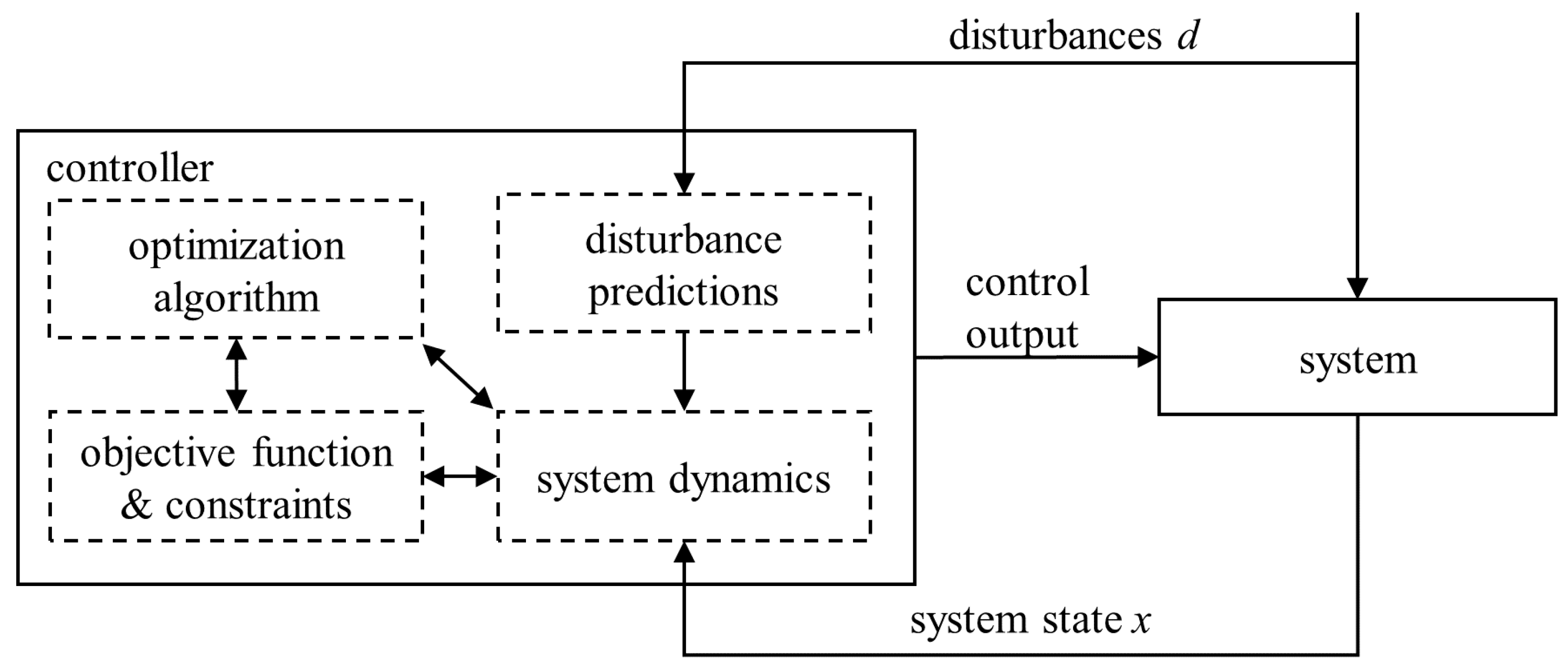
MPC is a model-based concept to control a system by solving an optimization problem under consideration of an objective function and possible constraints for each time instance of a defined prediction horizon. The general control concept is displayed in Figure 2.

The respective overall optimum control problem in case of the investigated building energy system is defined in Section 3.1. A detailed description of the system dynamics, the objective function, and the algorithm applied for weather forecasting is presented in the following subsections.

3.1. Definition of the Optimal Control Problem

The MPC aims to minimize an objective function J by prediction of the system behavior [34]. Within this article, this function represents the operational costs of the heat pump. The objective function J sums up the cost function ϕ in each time interval k of the prediction horizon N. In order to determine the mathematically optimal control sequence within an upcoming control horizon, an optimal control problem resulting from the system dynamics, the objective function, and the constraints have to be solved at every time step n [35]. A discretized definition of the optimum control problem is defined by the Equations (3)–(6) [36]:

$$J_N\left(n,x_0,u(·)\right):={\displaystyle \sum }_{k=0}^{N–1} \varnothing \left(n+k,x\left(k,x_0\right),u\left(k\right)\right) \mathrm{objective}\mathrm{function},$$

(3)

$$x\left(0,x_0\right)= x_0, x\left(k+1, x_0\right)=f\left(x\left(k,x_0\right)\right), u\left(k\right)\mathrm{system}\mathrm{dynamics},$$

(4)

$$Y:=\{\left(x,u\right)\in X \times U| x\in X, u\in U\}\mathrm{constraints},$$

(5)

$$\left(x_u\left(k, x_0\right),u\left(k\right)\right)\in Y\mathrm{for}\mathrm{all}k=0,\dots ,N-1,x_u\left(N,x_0\right)\in X\mathrm{constraints}.$$

(6)

The quantities X and U represent the possible system states x and the allowed range of the control vector u. Y represents the set of all allowed combinations.

The definition of the system dynamics, the objective function and the applied forecasting algorithm are described in the following sections. Constraints are considered by including them into the objective function. This constraint softening assures convergence of the optimization algorithm [33,37].

3.2. System Dynamics

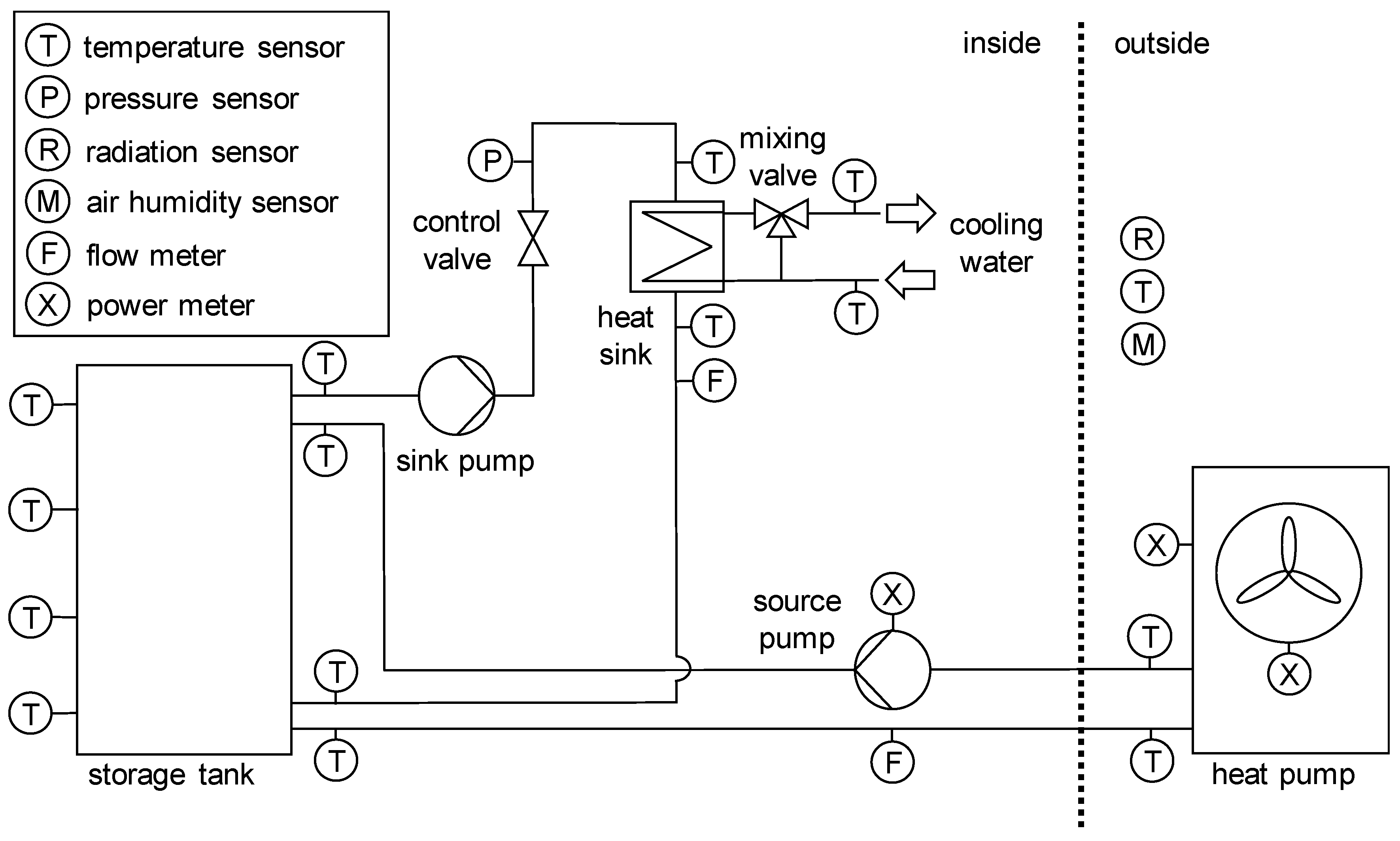
System dynamics are represented by a state space model. The model simplifies the test rig and the associated building model to four differential equations. A low complexity of the state space model is necessary for reducing the computational effort of real-time optimization.

The differential equations enable a dynamic calculation of the heating water, the floor heating system, and the building zone [28]. The simplified model considers the thermal capacities of the building, heat transfer between the mentioned zones, heat transfer to the ambient and heat gains by residents, electronics, and solar irradiation. The application of a state observer has been dispensed. The state space model is discretized by the explicit Euler method with a time step size of 300 s, which represents a compromise between computational effort and numerical convergence.

3.3. Objective Function and Optimization

The objective of the MPC optimization is to minimize the energy costs. Costs of the grid purchase of electric energy c_gp are considered to be 0.293 €/kWh, which was a typical value for a single-family house in Germany in 2018 [38]. In order to match the assumptions of the short-term measurements, PV energy grid feed-in c_fi is refunded at 0.122 €/kWh [28]. Next to these cost factors, PV curtailment is considered by additional costs c_cu = c_fi. In German PV-systems, the PV generation generally needs to be limited if PV power generation is close to its maximum capacity and PV self-consumption is low. The net grid feed-in maximum is limited to 70% of the maximum PV plant power P_PV,max. If the feed-in would exceed this level, the PV plant power is curtailed in order to prevent high public grid voltage.

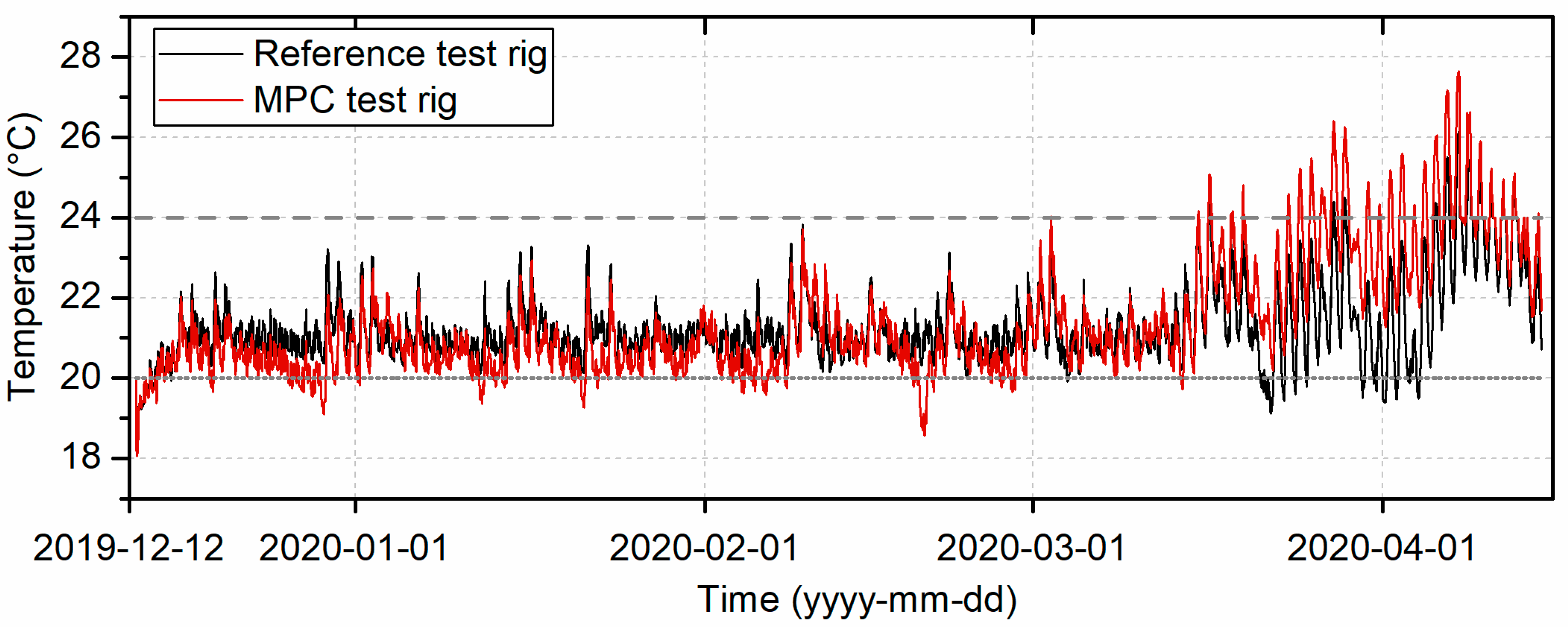
In addition to the energy cost factors, constraints are included into the objective function. These constraints aim to define the desired building zone temperature which is limited by a minimum comfort temperature of 20 °C and a maximum comfort temperature of 24 °C.

Comfort limit violation is considered by a penalty cost factor c_con. Undercutting the lower comfort limit ΔT is penalized by 0.5 €/Kh. As the exceedance of the upper comfort limit could be reduced by active ventilation in real systems, a factor of 0.1 €/Kh is applied on upper boundary exceedance within optimization. Thus, a constant violation of the thermal comfort boundaries is prevented, while a slight deviation in case of otherwise inefficient operation conditions is possible.

The resulting objective function is summarized by:

$$\begin{array}{l}\mathrm{J}={\displaystyle \sum }_{k=0}^{N–1}(\max \left(–P_{\mathrm{res}}\left(k\right),0\right)c_{gp}\Delta t–\max \left(P_{\mathrm{res}}\left(k\right),0\right)c_{fi}\Delta t+\max \left(P_{res}\left(k\right),0.7P_{\mathrm{PV},\max },0\right)c_{\mathrm{cu}}\Delta t\\ +c_{\mathrm{con}}\Delta T\left(k\right)\Delta t)\end{array}$$

(7)

with the control interval duration Δt of 900 s. The residual electric load

$$P_{\mathrm{res}}\left(k\right)=P_{\mathrm{PV}}\left(k\right) – P_{\mathrm{b}}\left(k\right) – u\left(k\right)P_{\mathrm{el},\mathrm{nom}}\left(T_{\mathrm{amb}}\left(k\right), T_{\mathrm{f}}\left(k\right)\right)$$

(8)

considers the predictions of the PV power generation P_PV and the prediction of the electric building load P_b. The nominal electricity consumption by the heat pump P_el,nom is calculated depending on the ambient air temperature T_amb and the flow temperature T_f.

The resulting optimal control problem is solved by a steepest-descent line search algorithm including Armijo’s condition of sufficient descent [39]. Optimization was carried out every hour with a prediction horizon of 24 h and control time intervals of 15 min. Resulting control signals of 10% or less were reduced to zero, as the heat pumps are not able to generate heat at very low part load.

3.4. Forecasting Algorithm

An algorithm according to Florita and Henze [40] was applied for weather forecasting in order to ensure comparability to the previous publication [28]. The algorithm predicts the outdoor temperature and the global horizontal radiation by past measurement data. Measurement values of a 24 h, 48 h, and 72 h backshift in time were equally weighted in order to predict all respective time interval values of the next 24 h. Moreover, a so-called absolute deviation modification of 25% was applied for air temperature prediction in order to adapt to sudden changes of the weather [28,40].

Next to the weather prediction, the algorithm was applied to predict the electrical building load and the internal building heat gains. Forecasting of the PV power generation and of the solar building heat gains was carried out by feeding the solar irradiation forecast values into the respective system models.

4. Results and Discussion

Section 4 shows the results derived from the described long-term experiments. In the first subsection, the experimentally gained data are analyzed and the findings are discussed. Based on that, the results are compared to existing short-term investigations in Section 4.2.

4.1. Experimental Results

In the first 24 h of the experiment, both test rigs apply the reference control, while a first prediction for the MPC is generated. A balance of heat generation and electrical energy consumption of the heat pumps during this period shows the comparability of the plants. Heat generation by the heat pumps within the starting period differs by 0.8%, while the deviation in electrical energy consumption amounts to 0.2%. The heat demand of the buildings and thus the heat transferred to the cooling network deviates by 0.3% comparing both test rigs. After 24 h, one out of the two heat pumps is controlled by the MPC.

Before the test phase can be examined more closely, a characterization of the weather is necessary. Figure 3 depicts the outside air-temperature which is influenced by high solar irradiation in the second half of March and in April. The same applies to the building zone temperatures which are displayed in Figure 4. A complete summary of the measured weather data can be found in Appendix A.

Figure 4 shows that both control concepts are able to set a comfortable building zone temperature for most of the experiment time. However, increased comfort limit exceedance occurs within the MPC controlled test rig. In case of an exceedance of the lower comfort limit, this is caused by drops in the ambient air temperature which were not predicted by the applied forecasting algorithm. Yet, the control concept is able to adapt the heat generation so that the lower limit is not undercut by more than 1 K in common operation. The only exception occurs on 19^th and 20^th of February, when the cooling system of the MPC test rig has shown malfunction and heat could not be transferred out of the test rig. Consequently, the simulated building was not heated any more. Although this also led to inefficient heat pump operation by high flow temperatures in the MPC test rig, the stability of the controller was demonstrated when the cooling system restarted operation.

In the second half of March and in April, the building zone temperatures partly exceed the upper comfort limit. Again, the MPC test rig shows a lower resident comfort, as the prediction algorithm needed up to 3 days to adapt to the unforeseen high global irradiation and outdoor temperatures. The comfort level could, however, be further improved by more accurate forecasting algorithms [41] or external and regional weather forecasting. Next to the forecasting error, the system cannot be cooled down by the controller actively and passive cooling during the night is overestimated. The state space system model does not include the thermal capacity of surrounding walls, as heat losses to the ambient are calculated by heat transmission coefficients for reasons of computational effort.

In total, the MPC test rig heat pump generated 1.1% more heat than the reference test rig heat pump during the 125 test days. However, the MPC controlled heat pump consumed 4.1% less electrical energy, as the heat pump COP was increased by 5.4%. In addition, the MPC algorithm more than doubled the PV electricity self-consumption and PV curtailment was reduced by 73.5%. Consequently, energy costs of the heat pump operation were reduced by 9.0%.

Table 1. Summary of experimental results.

Parameter	Reference	MPC	Rel. Deviation
Heat pump heat generation	4600 kWh	4648 kWh	+1.1%
Heat pump el. consumption	1032 kWh	990 kWh	−4.1%
Heat pump COP	4.46	4.70	+5.4%
PV electric energy generation	1473 kWh	1473 kWh	-
PV self-consumption	575.3 kWh	655.6 kWh	+14.0%
Heat pump: PV self-consumption	74.6 kWh	154.9 kWh	+107.7%
Heat pump: Electricity costs	289.7 €	263.5 €	−9.0%

sums up the experimental results.

The energetic and monetary advantages are based on a time shift of heat generation within the measurement days. The average load shifting is depicted in Figure 5.

As the reference control set point depends on the outdoor temperature, the average consumption of electric energy within the reference test rig is similar to a sinusoidal curve. The heat pump mainly generates heat in the night and morning hours. However, outdoor air temperatures and the coefficient of performance of an air-source heat pump are generally low within that time range. In contrast, the MPC algorithm shifts the main operation time of the heat pump towards the time from 10 am to 5 pm, with generally high outdoor temperatures and PV electricity generation on a daily basis. Nevertheless, unnecessary heating and high heat pump flow temperatures were avoided within the MPC test rig by means of a constant and low heat generation during the night.

The experiment confirms the general simulation results in literature, which state that PV self-consumption by heat pumps is increased by MPC [19]. Cost savings achieved by simulation studies [8,17,19] were missed by a few percentage points only, although perfect forecasting of real weather is almost impossible by algorithms based on local data. While savings reported of 12% by Kajgaard et al. [8] or of 13–15% by Salpakari and Lund [17] could not be reproduced, the range of 6% to 11% given by Fischer et al. [19] matches the experimental results presented within this study. It should be noted that the systems described in the literature partly consider different reference control concepts or take into account domestic hot water preparation.

Moreover, the experimental results in this study agree with literature short-term experimental results mentioned in the introduction. Measurements conducted by Péan et al. [27] showed reduced electrical energy consumption of 8.5% by application of MPC while heat generation was increased by 3.8%. Frison et al. [26] reported cost savings of 3.1% when the MPC focuses on grid-supportive operation. Thus, the presented long-term experiment also confirms short-term experimental results in the scientific literature. However, the results differ from previously published short-term experiment results of the same experimental setup [28], which needs to be discussed in the following section.

4.2. Comparison of Short- and Long-Term Experiments

Within the short-term measurements, which were performed in the heating season of 2019 from February to April, high average energy cost savings of 34.0% were achieved [28]. The average increase in PV self-consumption was 235%, while the electric energy consumption was reduced by 19.7% by the application of an MPC. These results could be achieved, as average global irradiation was already high in the test periods selected in February 2019 and the heat demand was still high during the March and April 2019 measurements.

Within the measurement presented in this study, the average solar irradiation and consequently the average difference between the minimum and maximum outside air temperature was low from December 2019 to February 2020. However, these weather conditions resulted in a low cost saving potential of MPC, while these months show the lowest outside air temperatures and consequently represent the main heat demand of the heating season. This is depicted in Figure 6 and Figure 7.

The figures show that the potential of increasing the self-consumption of renewable solar energy and of reducing the electric energy consumption in single-family homes strongly depends on the weather conditions. As already stated by Fischer and Madani [18], the seasonal discrepancy between the heat demand and solar irradiation limits both the PV self-consumption and the potential of applying an MPC. However, the test results still show that the MPC of residential heat pumps is economically viable and able to reduce electrical energy consumption. The MPC reduced the operating costs of the heat pump in every month. From December to February, these savings amount to an average value of 8.2%. In March, the lowest reduction of 4.9% was achieved due to excessive heat generation in the MPC test rig. The highest relative savings of 42.1% occurred in April. The discussion shows that the results significantly differ by repeating the measurement in a different heating period with lower ambient temperatures and higher solar irradiation within the colder months of the year.

5. Conclusions

Within this article, the model predictive control of an air-source heat pump in residential systems is compared to a current reference control. For the first time, the evaluation of the controller was performed over a period of several months with comparison to a reference test rig.

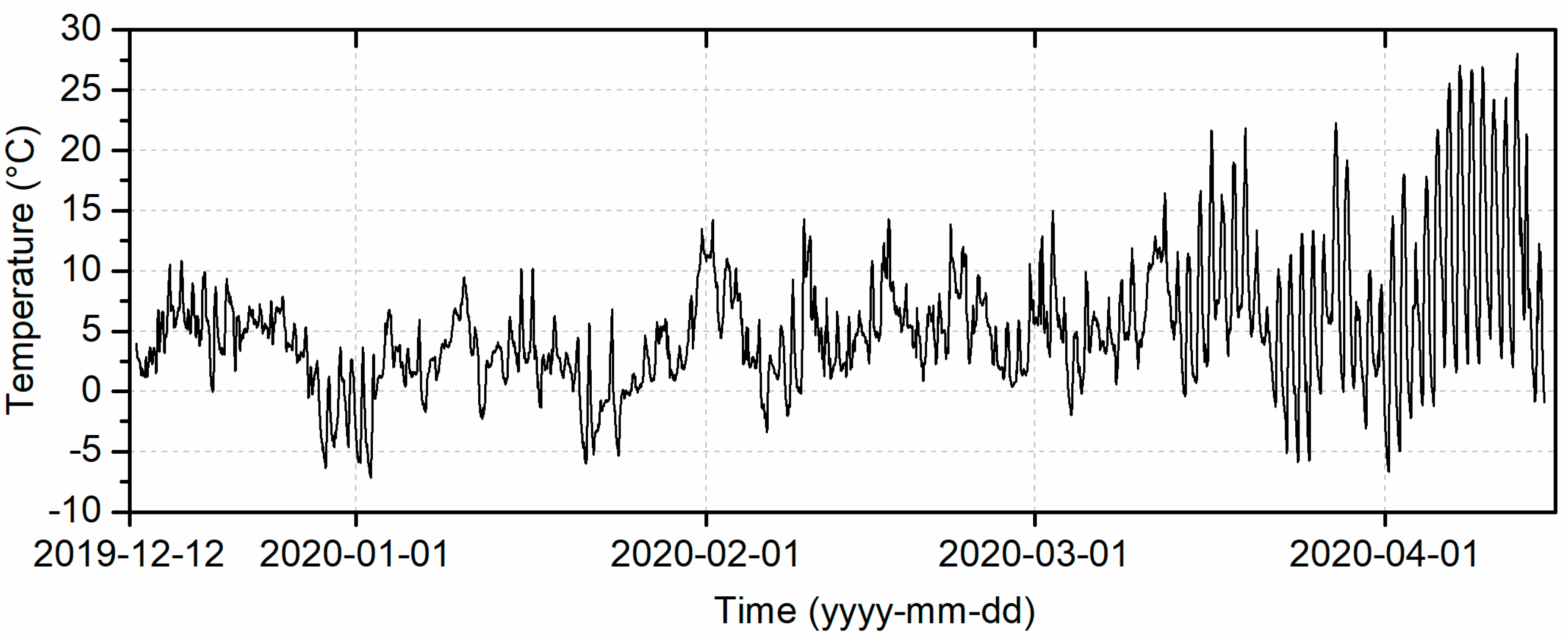
For this purpose, two identical test systems were set up, each with one heat pump. One of the heat pumps was controlled by the reference control concept, the other one by an economic MPC algorithm operating in real-time. The heat pumps operate under the influence of real weather conditions. The weather further impacts the identical building models, each one belonging to one of the test rigs. The building models specify the heat consumption in the test systems. The experimental test rig comprising two devices that are identical in construction operating under real weather conditions and considering photovoltaics represents a novelty compared to available experimental setups in the present literature.

An experiment was conducted from December 2019 to April 2020 to show to which extent an MPC is able to increase PV electricity self-consumption to reduce the heat pump electrical energy consumption and energy costs.

The main results are listed in the following:

• The applicability and stability of model predictive heat pump control was shown for the major part of one heating season.
• The residents’ thermal comfort was slightly reduced, while the heat generation was increased by the application of an MPC.
• The heat pump COP was enhanced by 5.4% in comparison to the reference.
• The electrical energy consumption of the heat pump was reduced by 4.1%.
• The PV electricity self-consumption of the heat pump was improved by 107.7%.
• The energy costs of heat pump operation decreased by 9.0%.

The presented scientific data demonstrate that the promising results of short-term experiments by other authors [26,27] also arise in long-term experiments. In this regard, the experimental long term-study, that has been conducted in this work for the first time, confirms the findings of simulation studies [8,17,19,42] too. A further comparison with short-term experiments conducted by application of the same test facility [28] proves the importance of long-term experiments and shows the dependence of the results on the weather. Hence, in future studies, the effect of using more accurate forecasting algorithms or external and regional weather forecasting on the advantages of the MPC and on the comfort level has to be investigated.

As the potential of MPC was found to be especially high in the transition period of the year, future work will also focus on the combination of space heating and domestic hot water supply.

References

1. Pérez-Lombard, L.; Ortiz, J.; Pout, C. A review on buildings energy consumption information. Energy Build. 2008, 40, 394–398. [Google Scholar] [CrossRef]
2. Afram, A.; Janabi-Sharifi, F. Theory and applications of HVAC control systems—A review of model predictive control (MPC). Build. Environ. 2014, 72, 343–355. [Google Scholar] [CrossRef]
3. Salvadori, G.; Ferrari, L.; Romano, L.; Fantozzi, F. Use of CARNOT Toolbox to Evaluate the Impact of Building Automation and Control Systems on Energy and CO2 Emission Savings. In Proceedings of the 2020 IEEE International Conference on Environment and Electrical Engineering and 2020 IEEE Industrial and Commercial Power Systems Europe (EEEIC/I&CPS Europe), Madrid, Spain, 9–12 June 2020. [Google Scholar] [CrossRef]
4. Killian, M.; Kozek, M. Ten questions concerning model predictive control for energy efficient buildings. Build. Environ. 2016, 105, 403–412. [Google Scholar] [CrossRef]
5. Oldewurtel, F.; Parisio, A.; Jones, C.N.; Gyalistras, D.; Gwerder, M.; Stauch, V.; Lehmann, B.; Morari, M. Use of model predictive control and weather forecasts for energy efficient building climate control. Energy Build. 2012, 45, 15–27. [Google Scholar] [CrossRef] [Green Version]
6. Péan, T.Q.; Salom, J.; Costa-Castello, R. Review of control strategies for improving the energy flexibility provided by heat pump systems in buildings. J. Process Control 2019, 74, 35–49. [Google Scholar] [CrossRef]
7. Felten, B.; Weber, C. The value (s) of flexible heat pumps—Assessment of technical and economic conditions. Appl. Energy 2018, 228, 1292–1319. [Google Scholar] [CrossRef]
8. Kajgaard, M.U.; Mogensen, J.; Wittendorff, A.; Veress, A.T.; Biegel, B. Model predictive control of domestic heat pump. In Proceedings of the 2013 IEEE American Control Conference, Washington, DC, USA, 17–19 June 2013. [Google Scholar] [CrossRef]
9. Halvgaard, R.; Poulsen, N.K.; Madsen, H.; Jørgensen, J.B. Economic model predictive control for building climate control in a smart grid. In Proceedings of the 2012 IEEE PES Innovative Smart Grid Technologies (ISGT), Washington, DC, USA, 16–20 January 2012. [Google Scholar] [CrossRef]
10. Bechtel, S.; Rafii-Tabrizi, S.; Scholzen, F.; Hadji-Minaglou, J.-R.; Maas, S. Influence of thermal energy storage and heat pump parametrization for demand-side-management in a nearly-zero-energy-building using model predictive control. Energy Build. 2020, 226, 110364. [Google Scholar] [CrossRef]
11. Gao, J.; Huang, G.; Xu, X. An optimization strategy for the control of small capacity heat pump integrated air-conditioning system. Energy Convers. Manag. 2016, 119, 1–13. [Google Scholar] [CrossRef] [Green Version]
12. Ruusu, R.; Cao, S.; Delgado, B.M.; Hasan, A. Direct quantification of multiple-source energy flexibility in a residential building using a new model predictive high-level controller. Energy Convers. Manag. 2019, 180, 1109–2239. [Google Scholar] [CrossRef]
13. Bruni, G.; Cordiner, S.; Mulone, V.; Rocco, V.; Spagnolo, F. A study on the energy management in domestic micro-grids based on Model Predictive Control strategies. Energy Convers. Manag. 2015, 102, 50–58. [Google Scholar] [CrossRef]
14. Toub, M.; Reddy, C.R.; Razmara, M.; Shahbakhti, M.; Robinett III, R.D.; Aniba, G. Model-based predictive control for optimal MicroCSP operation integrated with building HVAC systems. Energy Convers. Manag. 2019, 199, 111924. [Google Scholar] [CrossRef]
15. Angenendt, G.; Zurmühlen, S.; Rücker, F.; Axelsen, H.; Sauer, D.U. Optimization and operation of integrated homes with photovoltaic battery energy storage systems and power-to-heat coupling. Energy Convers. Manag. X 2019, 1, 100005. [Google Scholar] [CrossRef]
16. Franco, A.; Fantozzi, F. Experimental analysis of a self consumption strategy for residential building: The integration of PV system and geothermal heat pump. Renew. Energy 2016, 86, 1075–1085. [Google Scholar] [CrossRef]
17. Salpakari, J.; Lund, P. Optimal and rule-based control strategies for energy flexibility in buildings with PV. Appl. Energy 2016, 161, 425–436. [Google Scholar] [CrossRef] [Green Version]
18. Fischer, D.; Madani, H. On heat pumps in smart grids: A review. Renew. Sustain. Energy Rev. 2017, 70, 342–357. [Google Scholar] [CrossRef] [Green Version]
19. Fischer, D.; Bernhardt, J.; Madani, H.; Wittwer, C. Comparison of control approaches for variable speed air source heat pumps considering time variable electricity prices and PV. Appl. Energy 2017, 204, 93–105. [Google Scholar] [CrossRef]
20. Rastegarpour, S.; Gros, S.; Ferrarini, L. MPC approaches for modulating air-to-water heat pumps in radiant-floor buildings. Control Eng. Pract. 2020, 95, 104209. [Google Scholar] [CrossRef]
21. Gelleschus, R.; Böttiger, M.; Stange, P.; Bocklisch, T. Comparison of optimization solvers in the model predictive control of a PV-battery-heat pump system. Energy Procedia 2018, 155, 524–535. [Google Scholar] [CrossRef]
22. Gelleschus, R.; Böttiger, M.; Bocklisch, T. Optimization-Based Control Concept with Feed-in and Demand Peak Shaving for a PV Battery Heat Pump Heat Storage System. Energies 2019, 12, 2098. [Google Scholar] [CrossRef] [Green Version]
23. Široký, J.; Oldewurtel, F.; Cigler, J.; Prívara, S. Experimental analysis of model predictive control for an energy efficient building heating system. Appl. Energy 2011, 88, 3079–3087. [Google Scholar] [CrossRef]
24. Privara, S.; Široký, J.; Ferkl, L.; Cigler, J. Model predictive control of a building heating system: The first experience. Energy Build. 2011, 43, 564–572. [Google Scholar] [CrossRef]
25. Joe, J.; Karava, P.; Hou, X.; Xiao, Y.; Hu, J. A distributed approach to model-predictive control of radiant comfort delivery systems in office spaces with localized thermal environments. Energy Build. 2018, 175, 173–188. [Google Scholar] [CrossRef]
26. Frison, L.; Kleinstück, M.; Engelmann, P. Model-predictive control for testing energy flexible heat pump operation within a Hardware-in-the-Loop setting. J. Phys. Conf. Ser. 2019, 1343, 12068. [Google Scholar] [CrossRef]
27. Péan, T.; Costa-Castelló, R.; Fuentes, E.; Salom, J. Experimental testing of variable speed heat pump control strategies for enhancing energy flexibility in buildings. IEEE Access 2019, 7, 37071–37087. [Google Scholar] [CrossRef]
28. Kuboth, S.; Heberle, F.; Weith, T.; Welzl, M.; König-Haagen, A.; Brüggemann, D. Experimental short-term investigation of model predictive heat pump control in residential buildings. Energy Build. 2019, 109444. [Google Scholar] [CrossRef]
29. Bosch Thermotechnik GmbH Buderus Deutschland, Planungsunterlage für den Fachmann Reversible Luft-Wasser-Wärmepumpe, Ausgabe 2014/09 Logatherm WPL … AR (In German): Leistungsbereich von 6 kW bis 14 kW. 2018. Available online: https://productsat.buderus.com/techdoc/Logatherm-WPL-AR/6720811620.pdf (accessed on 7 May 2019).
30. Dott, R.; Haller, M.Y.; Ruschenburg, J.; Ochs, F.; Bony, J. The Reference Framework for System Simulations of the IEA SHC Task 44/HPP Annex 38 Part B: Buildings and Space Heat Load; International Energy Agency (Solar Heating and Cooling Programme): 2013. Available online: https://task44.iea-shc.org/Data/Sites/1/publications/T44A38_Rep_C1_B_ReferenceBuildingDescription_Final_Revised_130906.pdf (accessed on 17 September 2020).
31. De Soto, W.; Klein, S.A.; Beckman, W.A. Improvement and validation of a model for photovoltaic array performance. Sol. Energy 2006, 80, 78–88. [Google Scholar] [CrossRef]
32. Taylor, J. Introduction to Error Analysis, the Study of Uncertainties in Physical Measurements, 2nd ed.; University Science Books: California, CA, USA, 1997. [Google Scholar]
33. Findeisen, R.; Allgöwer, F. An Introduction to Nonlinear Model Predictive Control. In Proceedings of the 21st Benelux Meeting on Systems and Control, Veldhoven, The Netherlands, 19–21 March 2002. [Google Scholar]
34. Rawlings, J.B.; Mayne, D.Q. Model Predictive Control. Theory and Design, 1st ed.; Nob Hill Publ: Madison, WI, USA, 2009. [Google Scholar]
35. Verhelst, C.; Logist, F.; van Impe, J.; Helsen, L. Study of the optimal control problem formulation for modulating air-to-water heat pumps connected to a residential floor heating system. Energy Build. 2012, 45, 43–53. [Google Scholar] [CrossRef]
36. Grüne, L.; Pannek, J. Nonlinear Model Predictive Control: Theory and Algorithms, 2nd ed.; Springer International Publishing: Cham, Switzerland, 2017. [Google Scholar]
37. Papageorgiou, M. Optimierung. Statische, Dynamische, Stochastische Verfahren für die Anwendung, 2nd ed.; Oldenbourg: München, Germany, 1996. [Google Scholar]
38. Wirth, H.; Schneider, K. Aktuelle Fakten zur Photovoltaik in Deutschland (in German). Fraunhofer ISE. 2015. Available online: https://www.ise.fraunhofer.de/content/dam/ise/de/documents/publications/studies/aktuelle-fakten-zur-photovoltaik-in-deutschland.pdf (accessed on 10 September 2020).
39. Armijo, L. Minimization of functions having Lipschitz continuous first partial derivatives. Pac. J. Math. 1966, 16, 1–3. [Google Scholar] [CrossRef] [Green Version]
40. Florita, A.R.; Henze, G.P. Comparison of short-term weather forecasting models for model predictive control. HVAC&R Res. 2009, 15, 835–853. [Google Scholar]
41. Kwak, Y.; Huh, J.-H. Development of a method of real-time building energy simulation for efficient predictive control. Energy Convers. Manag. 2016, 113, 220–229. [Google Scholar] [CrossRef]
42. Kuboth, S.; Heberle, F.; König-Haagen, A.; Brüggemann, D. Economic model predictive control of combined thermal and electric residential building energy systems. Appl. Energy 2019, 240, 372–385. [Google Scholar] [CrossRef]
Figure 1. Setup of one test rig including the main components and the sensor equipment.
Energies 13 06016 g001
Figure 2. Model predictive control concept (adapted from Findeisen and Allgöwer [33]).
Energies 13 06016 g002
Figure 3. Measured ambient air temperature.
Energies 13 06016 g003
Figure 4. Building zone temperatures and thermal comfort limits.
Energies 13 06016 g004
Figure 5. Hourly average values of the electrical energy consumption of the heat pumps.
Energies 13 06016 g005
Figure 6. (a) Monthly mean ambient temperature and daily heat demand in the reference test rig; (b) mean solar irradiation and mean daily temperature spread during the measurement.
Energies 13 06016 g006
Figure 7. Monthly increase in the heat pump coefficient of performance (COP) and the heat pump self-consumption of photovoltaics (PV) electricity by application of model predictive control (MPC) in the long-term experiment.
Energies 13 06016 g007