Black Start Restoration of Islanded Droop-Controlled Microgrids

Abstract

The electricity grid faces the possibility of outages due to extreme weather events, cyber-attack, and unexpected events. When these unwanted events occur, it is desired that electricity be restored as soon as possible to meet the power demands of critical loads. The microgrid approach to power restoration holds a lot of promise, since microgrids can operate in island mode. This paper presents a novel sequential restoration methodology for microgrid black start. The microgrid architecture considered is assumed to be operating in multi-master mode. The master distributed generators (DGs) are coordinated to operate together through droop control. Several operational constraints are formulated and linearized to realize a mixed-integer linear programming (MILP) problem. The method is studied on an islanded microgrid based on a modified IEEE 13 node test feeder. Detailed transient simulation in PSCAD was used to verify the accuracy of the restoration methodology. The developed restoration method can maximize the energy restored while ensuring good voltage and frequency regulation, and ensure that power scheduling mismatch is shared in the desired proportion.

1. Introduction

The microgrid has been identified as one of the means to improve the resilience of the power system, through its ability to “island” and operate autonomously during disruptive situations [1,2]. Because of the microgrid’s ability to operate in island mode, it can significantly improve power system resilience during a blackout by providing electricity to critical loads. In August 2020, for instance, hot weather and wildfires led to a shortage of electricity supply in California; this caused the utilities to implement a rolling blackout. Several microgrids operated in island mode and freed up energy for other grid-connected customers, while other microgrids remained grid-connected and served as generating resources [3]. In several real-life scenarios, microgrids have been utilized to provide electricity in times of emergencies [4,5,6].

As discussed in [7], island operation of a microgrid is more challenging compared to grid-connected operation. Some challenges of microgrid island operation highlighted in [7] include smaller system size, higher distributed generator (DG) penetration and uncertainty, lower system inertia, unbalanced three-phase loading issues, and inability to use a traditional system analysis approach for an unbalanced microgrid system. Operating island microgrid under unbalanced load conditions has been shown to lead to instability [8]. These challenges call for clear consideration of the primary control for real-time voltage and frequency regulation, and the use of a systemic black start approach. Voltage and frequency regulation for microgrid island operation is usually accomplished through droop control [9,10,11,12].

Distribution system reconfiguration has widely been studied for restoration [13,14,15,16,17,18,19] through systematic mathematical formulation. These systematic formulations yield mathematical programming problems that can then be solved using an off-the-shelf solver. None of these formulations incorporated the use of droop control for islanded microgrids formation. Most of the works that considered the droop control of microgrid emergency operation (including the black start) did not formulate the black start operation of the studied microgrid systematically but rather were mostly rule-based and for concept verification through transient simulation and experimental studies [20,21,22,23]. However, as the size of the microgrid and the operation considerations increase, a rule-based approach becomes less reliable in finding a feasible and optimal (or near-optimal) solution. It is the purpose of this work to present a systematic approach to black start an islanded microgrid with droop considered as the primary control.

Because of changing system operating points as loads are restored sequentially during a black start, it is necessary to occasionally reset the primary control to ensure that the system is operating within the desired region and that power is being shared correctly. This resetting of the primary control is done by sending updated control parameter settings (like droop, load, and PQ DG settings) to the devices in the system. These updated settings are sent from the secondary and tertiary control layers, which are housed in the microgrid central controllers (MGCC) [24]. The MGCC, as an essential aspect of a microgrid, is expected to balance generation and load, coordinate load shedding when necessary, and regulate voltage and frequency [25].

In our earlier work [26], we presented black start restoration formulation for single master microgrids in which for each formed microgrid, one master DG is operated in isochronous mode (grid-forming mode), and other DGs in the same microgrid are operated in grid-following mode. Given a system with more than one isochronous DG, this led to the restoration of multiple smaller microgrids to keep the isochronous mode DGs isolated from each other. To restore a larger multi-master microgrid, this paper presents a black start formulation that incorporates the inter-operation of multiple masters DGs using droop control.

The main contribution of this paper includes the following:

• Propose a systematic black start formulation for the sequential restoration of islanded droop-controlled microgrids. To the best of the authors’ knowledge, this is the first systematic black start restoration formulation considering droop as the primary control.
• Show how to coordinate multiple grid-supporting (master/droop) and grid following (or PQ) DGs to dynamically configure microgrid instead of the multiple microgrids commonly considered in other systematic formulations. Coordination of the grid-supporting DGs to form a single microgrid, when possible, can help improve load balancing, resilience, redundancy, and better utilization of the DGs.
• Propose a zero-dispatch synchronization scheme for the grid-supporting DGs during the sequential build-up of the islanded microgrid and show how this can be mathematically composed into the restoration formulation.
• Validate the restoration approach through detailed electromagnetic transient program (EMTP) simulation in PSCAD and highlight some of the observations from the simulation such as restoration modeling limitations and suggestions on how these limitations can be solved.

The remaining part of this paper is organized as follows. Section 2 presents an overview of the droop control and droop reference operation scheme. Section 3 consists of an overview of the system components to be restored. In Section 4, an overview of the black process highlighting topology rules is presented, followed by the systematic mathematical formulation to realize a mixed-integer linear program (MILP) problem. Section 5 consists of a case study on an islanded microgrid based on the modified IEEE 13 node test feeder and solution verification using PSCAD simulation. This paper is concluded in Section 6 and areas for future work are identified.

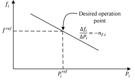
2. Droop Control Basics and Reference Operation

The power flow across a predominantly inductive line can be approximately decoupled such that the reactive power transfer is directly dependent on the voltage difference across the line and the active power is directly dependent on the power angle [10]. This decoupling ensures independent control of active and reactive power. In the distribution system with predominantly resistive lines, several methods, including inductive coupling, power transformation, and virtual impedance have been recommended to realize this power decoupling control [10,11,12]. The conventional droop control relies on this active and reactive power decoupling control. The black start restoration method developed in this paper assumes that the microgrid is controlled by conventional droop control with inductive coupling at the terminals of each droop-controlled DG.

Given a set of inverters in a microgrid, the equations describing the conventional droop control of the $i^{th}$ inverter is given as [9,27]:

$$f_i=f^{ref}-n_{f,i}(P_i-P_i^{ref}),$$

(1)

$$|{\overline{V}}_i|={|{\overline{V}}_i|}^{ref}-n_{v,i}(Q_i-Q_i^{ref}),$$

(2)

where $f^{ref}$ is the reference frequency in Hz assumed to be fixed and set to the nominal value for all droop inverters; $P_i^{ref}$ is the reference active power in per unit; $P_i$ is the active power output in per unit; $n_{f,i}$ is the frequency droop coefficient in Hz per unit power; ${|{\overline{V}}_i|}^{ref}$ is the reference voltage in per unit; $Q_i^{ref}$ is the reference reactive power in per unit; $|{\overline{V}}_i|$ is the output voltage in per unit; and $n_{v,i}$ is the voltage droop coefficient in per unit power.

Notice from (1) and (2), that if the output active power $P_i$ is equal to the reference active power setting, $P_i^{ref}$, then $f_i=f^{ref}$, and similarly if $Q_i=Q_i^{ref}$, then $|{\overline{V}}_i|={|{\overline{V}}_i|}^{ref}$. These two conditions are termed reference power operation throughout this paper. These conditions can be met or closely met when the droop reference power setpoints are chosen to match closely with the demanded power in the microgrid. Figure 1 below illustrates the reference power operation condition.

There is another way to express the droop equations in terms of idle frequency and voltage, as presented in [20]. However, the reference value-form of (1) and (2), though equivalent to the idle form, makes the calculation of the droop parameters easier by setting the reference frequency and voltage of each droop inverter at its reference (i.e., desired) active and reactive power setpoints, respectively.

3. Description of Islanded Microgrid to be Restored

The system is assumed to be an advanced distribution network (ADN) disconnected from the main grid with remote controlled switches (RCSs), conventional droop-controlled inverter-based DGs (grid-supporting DGs), dispatchable PQ inverter-based DGs (grid-feeding DGs), and switchable/non-switchable aggregated loads. Before the islanded microgrid is restored, we assume that an unforeseen emergency caused the system to be in a blackout state and thus, all resources in the system are de-energized to OFF state. In this completely de-energized state, the system would need to be black-started. An abstraction of the islanded distribution microgrid is shown in Figure 2.

Notice that in Figure 2, all the droop-controlled DGs are coupled to the distribution network via an inductor to enable active and reactive power decoupling. A two-way communication network is assumed to exist between the MGCC and the various devices in the system to facilitate status probing and setpoint corrections by the MGCC. The higher-level control (secondary and tertiary levels) are assumed to be executed by the MGCC, which sends set points to the DGs via a communication network.

4. Formulation of Black Start Restoration for Droop-Controlled Microgrid

In this section, an overview of the multi-master black start restoration is presented. This is followed by the detailed mixed-integer linear programming (MILP) model of the proposed restoration method. This MILP model starts by introducing the objective function followed by all the constraint equations. In the microgrid system considered, the objective function, constraint equations, and computation engine are expected to be stored and executed in the MGCC.

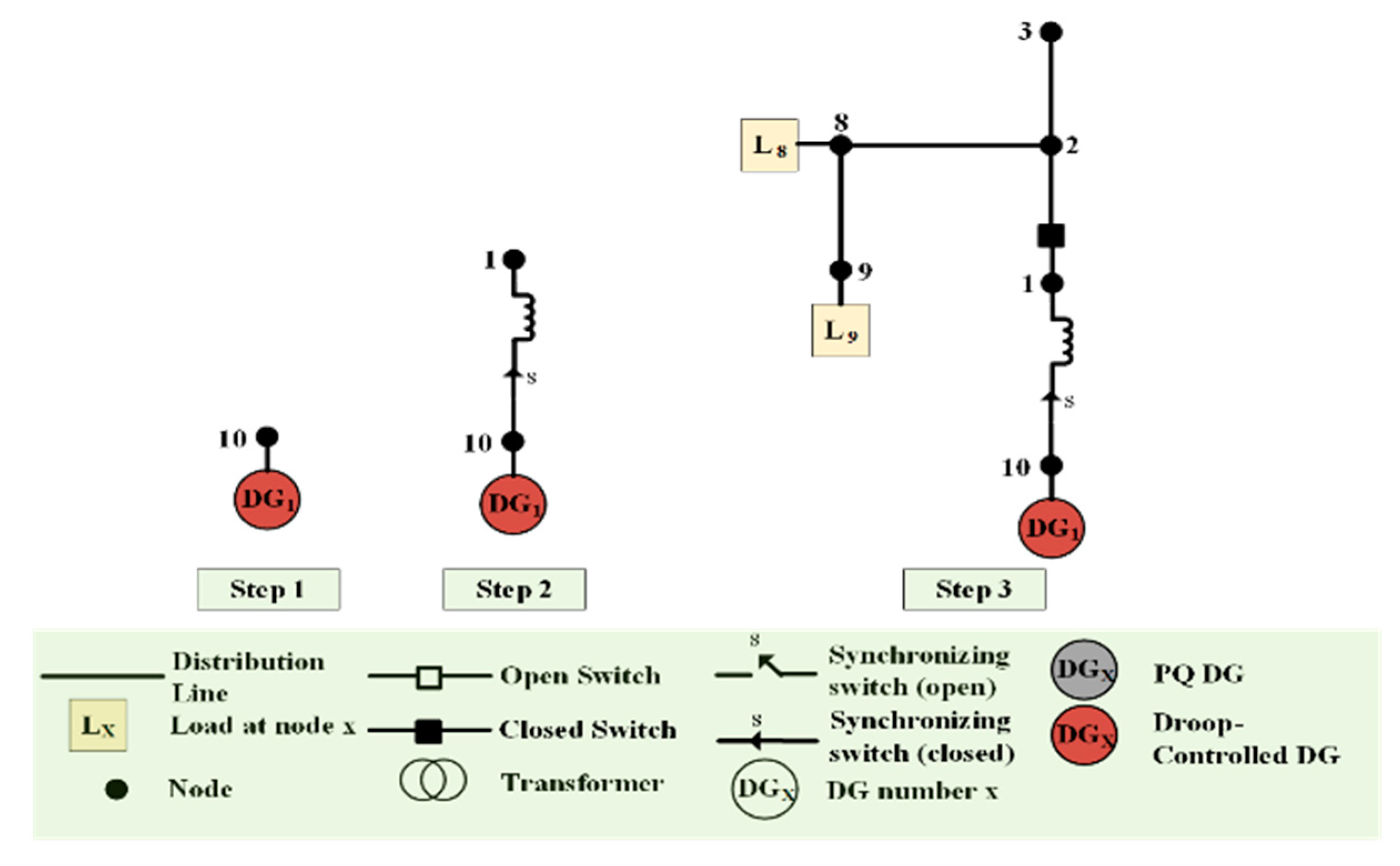
4.1. Overview of the Black Start Process

In multi-master mode, one or more grid-supporting DGs operating in droop mode are controlled to provide voltage reference for the system. Consider the 14-node distribution system in Figure 3 that needs to be restored after a blackout.

The goal is to restore the system and share the loads among the DGs. There are two three-phase grid-supporting DGs at nodes 10 and 14 which can act as a master for the system. There have been studies on sectionalizing distribution systems into multiple microgrids during restoration [13,15,16,17], however, interconnecting the multiple microgrids may become a challenge due to synchronization requirements, which we will show how to overcome below. Interconnected microgrids or forming larger microgrid will likely offer better reliability, load balancing, and energy coordination.

To solve the issue of synchronization of multiple microgrids, let us assume that the entire system starts expanding from one node, called a “build-up” node, with a grid supporting DG, and then connects with the other DGs as the build-up gets to the respective DG nodes. The following steps show an example build-up of the above 14-node islanded system for a black start restoration.

4.1.1. Step 1, 2, and 3

From Figure 3, nodes 10 and 14 are the nodes that are connected to droop-controlled DGs, therefore one of these two nodes can be chosen as a start-up node since the islanded system needs at least one master DG at any given time. Consider Figure 4 below. Let us assume that the central controller for the restoration chooses bus 10 as the build-up node after solving for the optimal system restoration sequence. Thus, the DG at node 10 is energized at the first restoration step as shown in Figure 4.

In step 2, the synchronizing switch of DG 1 is closed and node 1 becomes energized (in this step, the synchronizing switch is connecting to an unenergized system, therefore, there is no need for a synchronization check).

In step 3, the switch on the distribution line between nodes 1 to 2 is energized, leading to nodes 2, 3, 8, and 9 to become energized automatically since lines 2 to 3, 2 to 8, and 8 to 9 are non-switchable lines. In addition loads L8 and L9 are energized as well.

4.1.2. Step 4 and 5

In step 4, the line between nodes 3 and 5 is energized, which automatically energizes nodes 4, 5, 6, and 7. In addition, DG 2 is synchronized to the system and load L4 is energized too. The topology of the microgrid in this step is shown in Figure 5a.

Finally, in step 5, the droop-controlled DG at node 14 is synchronized to the system as shown in Figure 5b. For a stable connection, a precise synchronization method should be implemented in this droop-controlled DG. Even though the PQ DG needs to be synchronized as well, the synchronization of a droop-controlled DG is more critical since it is responsive to changes in the frequency and voltage of the microgrid.

However, if two microgrids were restored in parallel with each droop-controlled DG acting as a master for each microgrid, interconnecting both microgrids could become an issue. This is depicted in Figure 6. The boundary switch between the two microgrids at nodes 3 and 5 will not be able to adjust the frequency, voltage magnitude, and phase of both nodes for smooth synchronization. This is the motivation for building the microgrid from a single build-up node and then synchronizing each DG to the microgrid at their respective nodes since each DG is expected to have synchronization check capability.

In the subsections that follow, a mathematical model for the above multi-master black start restoration is formulated as a mixed-integer linear programming (MILP) problem. The flowchart of Figure 7 provides an overview of the proposed methodology. The symbols and parameters of the method are shown in

Table 1. Symbols and parameters of the proposed restoration method.

Sets
$n\left(A\right)$	The number of elements in set A
$B,B^S,B^F,C$	Set of branches, switchable and damaged branches, set of switchable branches between bus blocks
$G,G^{BS},G^{Dr},G^F,G^{PQ}$	Set of all DGs, subset of black start DGs, subset of droop-controlled DGs, subset of damaged DGs, subset of PQ DGs
$L,L^S,L^F$	Set of loads, subset of switchable loads, and subset of damaged load
$T$	Set of time steps $\left\{1,2,\dots ,N_T\right\}$ and $n\left(T\right)=N_T$
$N_p,N,K$	Set of phase nodes, nodes, bus blocks, $n\left(N_p\right)\ge n\left(N\right)\ge n\left(K\right)$
Binary Decision Variables (1–Energized, 0–Not Energized)
${\widehat{x}}_{i,t}^N,{\widehat{x}}_{j,t}^K$	Energization status of node $i$ at time step $t$, energization status of bus block $j$ at time step $t$
${\widehat{x}}_{g,t}^G$	Energization status of DG $g$ at time step $t$
${\widehat{x}}_{ij,t}^{BR},{\widehat{x}}_{ij,t}^K$	Energization status of line $\left(i,j\right)$ at time step, $t$, where $\left(i,j\right)\in B,C$ respectively
${\widehat{x}}_{l,t}^L$	Energization status of load $l$ at time step $t$
Continuous Decision Variables
$a,b,orc$	Used as subscript or superscript to denote variable or parameter in phase a, b or c respectively
${\widehat{P}}_{ph,k,t}^{dg}$, ${\widehat{Q}}_{ph,k,t}^{dg}$	Active and reactive power output of PQ DG $k$ at step $t$ and phase $ph\in \left\{a,b,c\right\}$
${\widehat{V}}_{n,t}^{re}$, ${\widehat{V}}_{n,t}^{im}$	Real and imaginary part of three-phase nodal voltage vector of node $n$ at step $t$
${\widehat{V}}_{n,t}^{re,ph}$, ${\widehat{V}}_{n,t}^{im,ph}$	Real and imaginary part of nodal voltage of node $n$ at step $t$ and phase $ph$
$n_{v,g,t}$	Voltage droop co-efficient of DG $g$, $g\in G^{Dr}$ at step $t$
$n_{f,g,t}$	Frequency droop co-efficient of DG $g$, $g\in G^{Dr}$ at step $t$
${\widehat{P}}_{ph,k,t}^{ref},{\widehat{Q}}_{ph,k,t}^{ref}$	Droop reference active and reactive power output of DG $k$ at step $t$, $k\in G^{Dr}$
${\widehat{P}}_{ph,l,t},{\widehat{Q}}_{ph,l,t}$	Nominal active and reactive power demand of load $l$, phase $ph$, at time step $t$
Parameters
$M$	A large number chosen deliberately to manipulate the constraint equations
$\Delta t$	time interval between restoration steps and is assumed to be a constant value for all intervals
$P_g^{G,ramp},Q_g^{G,ramp}$	Maximum absolute value of differential active and reactive power output of DG $g$ for each time step (DG ramp rate)
$P_g^{min},P_g^{max}$	Minimum and maximum active power output of DG $g$
$Q_g^{min},Q_g^{max}$	Minimum and maximum reactive power output of DG $g$
$P_{ph,l,t},Q_{ph,l,t}$	Nominal active and reactive power value of load $l$, phase $ph$, at time step $t$ (fixed to the same value for all time steps and is independent of whether the load has been restored or not)
$z_{i,j}=r_{i,j}+j{x}_{i,j}$	Impedance of line between nodes $i$ and $j$, and $y_{i,j}=\frac{1}{z_{i,j}}=g_{i,j}+j{b}_{i,j}$
$y_{i,j}^{sh}=g_{i,j}^{sh}+j{b}_{i,j}^{sh}$	Shunt admittance between nodes $i$ and $j$

. Decision variables are denoted with a hat. The formulation is a multi-step restoration approach that follows a similar sequence of the example presented in Figure 4 and Figure 5.

4.2. Objective Function

The objective function of the developed method is to maximize the energy restored in the time horizon under consideration while maintaining system operational constraints:

$$min-{\sum }_{t\in T}{\sum }_{l\in L}{\sum }_{ph\in \left\{a,b,c\right\}}{\widehat{P}}_{ph,l,t}.\Delta t,$$

(3)

where ${\widehat{P}}_{ph,l,t}={\widehat{x}}_{l,t}^L{P}_{ph,l,t}$. As defined in Table 1, ${\widehat{x}}_{l,t}^L$ is a binary variable which represents the energization status of the load $l$ at time step $t$, and $P_{ph,l,t}$ is the nominal value of load $l$ at time step $t$ for phase $ph$, $\Delta t$ is the time interval between steps and is assumed to be a constant value for all intervals.

The objective function of (3) is subject to the following operating constraints: initial sequencing constraints (Equations (4)–(6)), connectivity constraints (Equations (7)–(14)), synchronization enhancing constraints (Equations (15)–(22)), power flow constraints (Equations (30), (31), (41), (42), and (45)–(50)), DG and system operation constraints (Equations (51)–(54), (56)–(67)), and topology and sequencing constraints (Equations (68)–(72)). These constraints are discussed in the subsections that follow.

4.3. Initial Sequencing Constraints

The sequencing constraints ensure that the system builds up in the desired way. One node is selected as the build-up node by the dynamic optimization algorithm. These initial start-up conditions are expressed in Equations (4)–(6) below.

$${\sum }_{g\in \{G^{Dr}n{G}^{BS}\}}{\widehat{x}}_{g,t}^G=1,{\sum }_{g\in \{G\backslash (G^{Dr}n{G}^{BS})\}}{\widehat{x}}_{g,t}^G=0,t=1,$$

(4)

$${\widehat{x}}_{ij,t}^{BR}=0,(i,j)\in B^S\backslash B^F,t=1,$$

(5)

$${\widehat{x}}_{ij,t}^{BR}=0,{\widehat{x}}_{g,t}^G=0,{\widehat{x}}_{l,t}^L=0,(i,j)\in B^F,g\in G^F,l\in L^F,t\in T,$$

(6)

The first sum in Equation (4) ensures that one black start droop-controlled DG is started at time step 1 at the build-up node and the second sum ensures that all other DGs are not connected. Equation (5) ensures that all switchable lines are turned off at time step 1. Equation (6) ensures that the status of all damaged resources are de-energized by setting them to 0 for all time steps.

4.4. Connectivity Constraints

Connectivity constraints help to ensure acceptable interconnection between elements in the system. The concepts of these connectivity constraints were adapted from [16,17] to suit the multi-master microgrid architecture. In general, we consider the following interconnection acceptable for each step of the restoration:

• Whenever a DG is energized, then that DG’s node must have been energized in the same or previous time step as the DG energization time step (Equation (7))
• Once any DG, branch, or load is energized, it cannot be de-energized (EQUATIONS (8), (11), and (14) respectively)
• Both nodes of an energized switchable branch must be energized (Equation (9)) and the status of non-switchable branches are the same with its two nodes (Equation (10))
• A switchable load can only be energized once its node is energized (Equation (12)) and a non-switchable load is automatically energized when its node is energized (Equation (13))

These interconnection requirements are enforced according to the constraint equations below:

$${\widehat{x}}_{g,t}^G\le {\widehat{x}}_{g,t}^N,g\in G,t\in T,$$

(7)

$${\widehat{x}}_{g,t}^G-{\widehat{x}}_{g,t-1}^G\ge 0,g\in G,t\in T,$$

(8)

$${\widehat{x}}_{ij,t}^{BR}\le {\widehat{x}}_{i,t}^N,{\widehat{x}}_{ij,t}^{BR}\le {\widehat{x}}_{j,t}^N,\left(i,j\right)\in B^S\backslash B^F,t\in T,i,j\in N,$$

(9)

$${\widehat{x}}_{ij,t}^{BR}={\widehat{x}}_{i,t}^N,{\widehat{x}}_{ij,t}^{BR}={\widehat{x}}_{j,t}^N,\left(i,j\right)\in B\backslash B^S\backslash B^F,t\in T,i,j\in N,$$

(10)

$${\widehat{x}}_{ij,t}^{BR}-{\widehat{x}}_{ij,t-1}^{BR}\ge 0,\left(i,j\right)\in B^S\backslash B^F,t\in T,i,j\in N,$$

(11)

$${\widehat{x}}_{n,t}^L\le {\widehat{x}}_{n,t}^N,n\in L^S\backslash L^F,t\in T,$$

(12)

$${\widehat{x}}_{n,t}^L={\widehat{x}}_{n,t}^N,n\in L\backslash L^S\backslash L^F,t\in T,$$

(13)

$${\widehat{x}}_{n,t}^L-{\widehat{x}}_{n,t-1}^L\ge 0,n\in L^S\backslash L^F,t\in T,$$

(14)

4.5. Synchronization Enhancing Constraints

Connecting a grid-supporting DG to an already operating islanded microgrid is a complex interplay of all the controllers in the system, and because of the low inertia of the system, this can easily lead the system to instability. Conditions that can minimize angle, frequency, and voltage transients during synchronization of grid-supporting DGs can help enhance smooth synchronization. These conditions, which we call zero-dispatch synchronization, are identified as follows:

• At most one droop-controlled DG can be newly connected to the system per time step (Equation (15))
• “Freeze” the status/settings of every other element at any time step that a droop-controlled DG is synchronized to the system. This means that:
  • No additional load is restored at a synchronization time step (Equation (16)).
  • The status and dispatch settings of PQ DGs should remain the same as the previous time step just before the synchronization step (Equations (17)–(19)).
  • The active and reactive power reference settings of all droop DGs should remain the same as the previous time step just before the synchronization step, and the DG that is about to be synchronized to the system should do at zero power reference settings (Equations (20) and (21)). Equations (20) and (21) also ensure that the synchronized DG is connected with a zero reference power since its reference power at the previous step would be set to zero according to the DG operation constraints.
  • The status of all branches should remain the same as the previous time step just before the synchronization step except for one branch that can connect the synchronizing DG to the system, that is, only the branch that connects the DG to the system is allowed to change from “OFF” to “ON” (Equation (22)) if it was not already energized.

$${\sum }_{g\in \{G^{Dr}\}}{\widehat{x}}_{g,t+1}^G-{\sum }_{g\in \{G^{Dr}\}}{\widehat{x}}_{g,t}^G\le 1,t\in T,$$

(15)

$${\widehat{x}}_{n,t+1}^L-{\widehat{x}}_{n,t}^L\le M\left(1-{\sum }_{g\in \{G^{Dr}\}}\left({\widehat{x}}_{g,t+1}^G-{\widehat{x}}_{g,t}^G\right)\right),n\in L,t\in T,$$

(16)

$${\widehat{x}}_{g,t+1}^G-{\widehat{x}}_{g,t}^G\le M\left(1-{\sum }_{g\in \{G^{Dr}\}}\left({\widehat{x}}_{g,t+1}^G-{\widehat{x}}_{g,t}^G\right)\right),g\in G^{PQ},t\in T,$$

(17)

$$\begin{array}{l}-M\left(1-{\sum }_{g\in \{G^{Dr}\}}\left({\widehat{x}}_{g,t+1}^G-{\widehat{x}}_{g,t}^G\right)\right)\le {\widehat{P}}_{ph,k,t+1}^{dg}-{\widehat{P}}_{ph,k,t}^{dg}\\ \le M\left(1-{\sum }_{g\in \{G^{Dr}\}}\left({\widehat{x}}_{g,t+1}^G-{\widehat{x}}_{g,t}^G\right)\right),k\in G^{PQ},t\in T,\end{array}$$

(18)

$$\begin{array}{l}-M\left(1-{\sum }_{g\in \{G^{Dr}\}}\left({\widehat{x}}_{g,t+1}^G-{\widehat{x}}_{g,t}^G\right)\right)\le {\widehat{Q}}_{ph,k,t+1}^{dg}-{\widehat{Q}}_{ph,k,t}^{dg}\\ \le M\left(1-{\sum }_{g\in \{G^{Dr}\}}\left({\widehat{x}}_{g,t+1}^G-{\widehat{x}}_{g,t}^G\right)\right),k\in G^{PQ},t\in T,\end{array}$$

(19)

$$\begin{array}{l}-M\left(1-{\sum }_{g\in \{G^{Dr}\}}\left({\widehat{x}}_{g,t+1}^G-{\widehat{x}}_{g,t}^G\right)\right)\le {\widehat{P}}_{ph,k,t+1}^{ref}-{\widehat{P}}_{ph,k,t}^{ref}\\ \le M\left(1-{\sum }_{g\in \{G^{Dr}\}}\left({\widehat{x}}_{g,t+1}^G-{\widehat{x}}_{g,t}^G\right)\right),k\in G^{Dr},t\in T,\end{array}$$

(20)

$$\begin{array}{l}-M\left(1-{\sum }_{g\in \{G^{Dr}\}}\left({\widehat{x}}_{g,t+1}^G-{\widehat{x}}_{g,t}^G\right)\right)\le {\widehat{Q}}_{ph,k,t+1}^{ref}-{\widehat{Q}}_{ph,k,t}^{ref}\\ \le M\left(1-{\sum }_{g\in \{G^{Dr}\}}\left({\widehat{x}}_{g,t+1}^G-{\widehat{x}}_{g,t}^G\right)\right),k\in G^{Dr},t\in T,\end{array}$$

(21)

$${\sum }_{\left(i,j\right)\in B}{\widehat{x}}_{ij,t+1}^{BR}-{\sum }_{\left(i,j\right)\in B}{\widehat{x}}_{ij,t}^{BR}\le 1+M\left(1-{\sum }_{g\in \{G^{Dr}\}}\left({\widehat{x}}_{g,t+1}^G-{\widehat{x}}_{g,t}^G\right)\right),t\in T,$$

(22)

4.6. Power Flow Constraints

The power flow constraints for an islanded microgrid with droop-controlled inverters are a bit tricky to derive. First, there is no bus to approximate as a slack bus. In addition, there are additional nodes at the droop-controlled DGs’ nodes before the inductor coupling which have to be considered in the power flow formulation. In this subsection, we adapt the linear power flow derivation using the current injection approach for a multi-time step restoration with switchable and non-switchable branches.

4.6.1. Kirchhoff’s Current Law (KCL) at each Node

For balanced three-phase systems, the power flow is usually represented in terms of balanced single-phase per unit equivalence as in [28]:

$$\overline{Y}\overline{V}=\overline{I},$$

(23)

where $\overline{Y}$ is the complex bus admittance matrix, $\overline{V}$ is the complex bus voltage vector and $\overline{I}$ is the complex current injection vector. Equation (23) is derived by the application of KCL at each node. For three-phase unbalanced systems, the $\overline{Y}$ is computed considering each phase as a node (each phase node) and the unbalanced branch and shunt admittances. Let $\overline{Y}=G+jB$, $\overline{V}=V^{re}+j{V}^{im}$, and $\overline{I}=I^{re}+j{I}^{im}$, then (23) can be separated into real and imaginary parts:

$$\left[\begin{array}{cc}G& -B\\ B& G\end{array}\right]\left[\begin{array}{c}{V}^{re}\\ V^{im}\end{array}\right]=\left[\begin{array}{c}{I}^{re}\\ I^{im}\end{array}\right],$$

(24)

Ideally (24) would represent the system physics for a single time step solution where the status of the branches is known. However, in the case of multi-time step restoration, the status of the branches is not known ahead of time until after the restoration solution is returned by the optimization solver. Therefore, the bus admittance matrix, $\overline{Y}=G+jB$, has to be modified to include branch energization status which would determine whether a given branch admittance should be included (or not included) in the bus admittance matrix.

First, we show how to include the energization status of branches into Equations (23) and (24) using a simple three-node power system and then generalize to an arbitrary number of nodes. Consider Figure 8 below:

In Figure 8, there are three nodes labeled 1, 2, and 3, and each is assumed to be a three-phase node. This means that the voltage of each node, labeled $V_1$, $V_2$, and $V_3$, are each complex vectors of length equal to three as well as the current injections. $y_{21}$ and $y_{21}^{sh}$ are each a 3 × 3 complex branch admittance matrix and shunt admittance matrix respectively between nodes 2 and 1. $y_{31}$ and $y_{31}^{sh}$ are each a 3 × 3 complex branch admittance matrix and shunt admittance matrix, respectively, between nodes 3 and 1. $x_{2,1}^{BR}=x_{1,2}^{BR}$, and is considered the binary energization status of the branch between nodes 2 and 1. Likewise, $x_{3,1}^{BR}=x_{1,3}^{BR}$, and is considered binary energization status of the branch between nodes 3 and 1.

Application of Kirchhoff’s current law at node 1 will depend on the energization status of $x_{1,2}^{BR}$ and $x_{1,3}^{BR}$, and can be written following the assumed current direction indicated by the arrows in Figure 8 as follows.

$$x_{1,2}^{BR}{y}_{21}\left(V_1-V_2\right)+x_{1,2}^{BR}\frac{y_{21}^{sh}}{2}{V}_1+x_{1,3}^{BR}{y}_{31}\left(V_1-V_3\right)+x_{1,3}^{BR}\frac{y_{31}^{sh}}{2}{V}_1=I_1,$$

(25)

Note that in (25), the multiplication of energization status and a matrix or vector is a scalar multiplication. Equation (25) can be rearranged as follows.

$$\left(x_{1,2}^{BR}{y}_{21}+x_{1,3}^{BR}{y}_{31}+x_{1,3}^{BR}\frac{y_{31}^{sh}}{2}\right)V_1+\left(-x_{1,2}^{BR}{y}_{21}\right)V_2+\left(-x_{1,3}^{BR}{y}_{31}\right)V_3=I_1,$$

(26)

Similar KCL Equations as (26) can be written for nodes 2 and 3. Equation (26) can be written in matrix form where X has been used to represent equivalent elements for the KCL at nodes 2 and 3.

$$\underset{Y(x^{BR})}{\underbrace{\left[\begin{array}{ccc}{x}_{1,2}^{BR}{y}_{21}+x_{1,3}^{BR}{y}_{31}+x_{1,3}^{BR}\frac{y_{31}^{sh}}{2}& -x_{1,2}^{BR}{y}_{21}& -x_{1,3}^{BR}{y}_{31}\\ X& X& X\\ X& X& X\end{array}\right]}}\left[\begin{array}{c}{V}_1\\ V_2\\ V_3\end{array}\right]=\left[\begin{array}{c}{I}_1\\ X\\ X\end{array}\right],$$

(27)

Notice that the coefficient matrix, which is the complex Y bus admittance matrix, is now a function of branch energization status. Note that $y_{nm}=g_{nm}+j{b}_{nm}$, $y_{nm}^{sh}=g_{nm}^{sh}+j{b}_{nm}^{sh}$, $V_n=V_n^{re}+j{V}_n^{im}$, and $I_n=I_n^{re}+j{I}_n^{im}$. Without the energization status, the off-diagonal term of the bus admittance matrix is given by $Y_{nm}=-y_{nm}$. Note that $Y_{nm}=G_{nm}+j{B}_{nm}$, $\therefore G_{nm}=-g_{nm}$, $B_{nm}=-b_{nm}$. Substituting $y_{nm}=g_{nm}+j{b}_{nm}$, $y_{nm}^{sh}=g_{nm}^{sh}+j{b}_{nm}^{sh}$, $V_n=V_n^{re}+j{V}_n^{im}$, $I_n=I_n^{re}+j{I}_n^{im}$ into (26) and separating the resulting expression into real and imaginary gives the following:

$$\begin{array}{c}{\sum }_{\begin{array}{c}k:k\in \left\{1,2,3\right\}\\ k\ne 1\end{array}}(G_{1,k}{V}_k^{re}-B_{1,k}{V}_k^{im})x_{1,k}^{BR}+{\sum }_{\begin{array}{c}k:k\in \left\{1,2,3\right\}\\ k\ne 1\end{array}}(-G_{1,k}{V}_1^{re}+\frac{g_{1,k}^{sh}}{2}{V}_1^{im})x_{1,k}^{BR}\\ -{\sum }_{\begin{array}{c}k:k\in \left\{1,2,3\right\}\\ k\ne 1\end{array}}(-B_{1,k}{V}_1^{re}+\frac{b_{1,k}^{sh}}{2}{V}_1^{im})x_{1,k}^{BR}=I_n^{re},\end{array}$$

(28)

$$\begin{array}{c}{\sum }_{\begin{array}{c}k:k\in \left\{1,2,3\right\}\\ k\ne 1\end{array}}(B_{1,k}{V}_k^{re}+G_{1,k}{V}_k^{im})x_{1,k}^{BR}+{\sum }_{\begin{array}{c}k:k\in \left\{1,2,3\right\}\\ k\ne 1\end{array}}(-B_{1,k}{V}_1^{re}+\frac{b_{1,k}^{sh}}{2}{V}_1^{im})x_{1,k}^{BR}\\ +{\sum }_{\begin{array}{c}k:k\in \left\{1,2,3\right\}\\ k\ne 1\end{array}}(-G_{1,k}{V}_1^{re}+\frac{g_{1,k}^{sh}}{2}{V}_1^{im})x_{1,k}^{BR}=I_n^{im},\end{array}$$

(29)

Equations (28) and (29) are the real and imaginary parts of Equation (26), respectively, in expanded form. The first summation terms in Equations (28) and (29) are the product terms due to the off-diagonal Y bus terms written in rectangular coordinate. The next two terms in Equations (28) and (29) are the product terms due to the leading diagonal terms of the Y bus matrix. Similar equations can be written for the KCL at nodes 2 and 3 of Figure 8.

We can generalize Equations (28) and (29) for an arbitrary node $n$ of a microgrid with sets of nodes $N$ as follows, with additional step subscript for the time step indicated by $t$ as follows:

$$\begin{array}{c}{\sum }_{\begin{array}{c}k:k\in N\\ k\ne n\end{array}}(G_{n,k}{\widehat{V}}_{k,t}^{re}-B_{n,k}{\widehat{V}}_{k,t}^{im}){\widehat{x}}_{n,k,t}^{BR}+{\sum }_{\begin{array}{c}k:k\in N\\ k\ne n\end{array}}(-G_{n,k}{\widehat{V}}_{n,t}^{re}+\frac{g_{n,k}^{sh}}{2}{\widehat{V}}_{n,t}^{re}){\widehat{x}}_{n,k,t}^{BR}\\ -\sum _{\begin{array}{c}k:k\in N\\ k\ne n\end{array}}(-B_{n,k}{\widehat{V}}_{n,t}^{im}+\frac{b_{n,k}^{sh}}{2}{\widehat{V}}_{n,t}^{im}){\widehat{x}}_{n,k,t}^{BR}={\widehat{I}}_{n,t}^{re}\left({\widehat{V}}_{n,t}^{re},{\widehat{V}}_{n,t}^{im}\right),\end{array}$$

(30)

$$\begin{array}{c}{\sum }_{\begin{array}{c}k:k\in N\\ k\ne n\end{array}}(B_{n,k}{\widehat{V}}_{k,t}^{re}+G_{n,k}{\widehat{V}}_{k,t}^{im}){\widehat{x}}_{n,k,t}^{BR}+{\sum }_{\begin{array}{c}k:k\in N\\ k\ne n\end{array}}(-B_{n,k}{\widehat{V}}_{n,t}^{re}+\frac{b_{n,k}^{sh}}{2}{\widehat{V}}_{n,t}^{re}){\widehat{x}}_{n,k,t}^{BR}\\ +\sum _{\begin{array}{c}k:k\in N\\ k\ne n\end{array}}(-G_{n,k}{\widehat{V}}_{n,t}^{im}+\frac{g_{n,k}^{sh}}{2}{\widehat{V}}_{n,t}^{im}){\widehat{x}}_{n,k,t}^{BR}={\widehat{I}}_{n,t}^{im}\left({\widehat{V}}_{n,t}^{re},{\widehat{V}}_{n,t}^{im}\right),\end{array}$$

(31)

where $G_{n,k}=-g_{n,k}$ ($g_{n,k}$ is a matrix that represents the real part of the branch admittance between nodes $n$ and $k$) and $B_{n,k}=-b_{n,k}$ ($b_{n,k}$ is a matrix that represents the imaginary part of the branch admittance between nodes $n$ and $k$). Note that ${\widehat{V}}_{n,t}^{re}={\left[{\widehat{V}}_{n,t}^{re,a}{\widehat{V}}_{n,t}^{re,b}{\widehat{V}}_{n,t}^{re,c}\right]}^T$, ${\widehat{V}}_{n,t}^{im}={\left[{\widehat{V}}_{n,t}^{im,a}{\widehat{V}}_{n,t}^{im,b}{\widehat{V}}_{n,t}^{im,c}\right]}^T$, and ${\widehat{I}}_{n,t}^{re}$ and ${\widehat{I}}_{n,t}^{im}$ are similarly defined as three-phase current vectors.

To specify the linear power flow constraint for the microgrid to be restored, (30) and (31) have to be defined as constraints for every node and every step of the restoration. Just like in (28) and (29), the first summation terms in Equations (30) and (31) are the product terms due to the off-diagonal Y bus terms written in rectangular coordinate. The next two terms in Equations (30) and (31) are the product terms due to the leading diagonal terms of the Y bus matrix. The right hand side (RHS) terms are the sum of the three-phase current injection vectors at each node. The left hand side (LHS) of Equations (30) and (31) present bilinear vector terms which are products of rectangular voltage vectors (continuous) and branch energization status (binary)—these terms are linearized by introducing new variables for each bilinear term as explained below.

Given the product of an arbitrary binary variable, $b$, and an arbitrary continuous variable, $x$, where $x$ is bounded below and above by $x_{min}$ and $x_{max}$, respectively. Introduce and replace this product with a new variable $z=bx$ wherever it is found in the model. We can linearize this product as follows by including constraints (32) and (33) in the model.

$$x_{min}\le x\le x_{max},$$

(32)

$$x_{min}b\le z\le x_{max}b,x_{min}\left(1-b\right)\le x-z\le x_{max}\left(1-b\right),$$

(33)

4.6.2. Current Injection at Each Node

At any given generic phase $ph$ and node $n$, with power injections $P_{ph,n,t}^{inj}+j{Q}_{ph,n,t}^{inj}$, the current injection per phase can be written as follows in terms of the phase power injection and phase node voltage:

$${\overline{I}}_{ph,n,t}={\widehat{I}}_{n,t}^{re,ph}+j{\widehat{I}}_{n,t}^{im,ph}=\frac{P_{ph,n,t}^{inj}-j{Q}_{ph,n,t}^{inj}}{{\widehat{V}}_{n,t}^{re,ph}-j{\widehat{V}}_{n,t}^{im,ph}},$$

(34)

Equation (34) is derived from the complex power equation, which means that the current is equal to the complex conjugate of complex power divided by the complex conjugate of voltage. Separating the RHS of (34) into real and imaginary parts gives the following:

$${\widehat{I}}_{n,t}^{re,ph}=\frac{P_{ph,n,t}^{inj}{\widehat{V}}_{n,t}^{re,ph}+Q_{ph,n,t}^{inj}{\widehat{V}}_{n,t}^{im,ph}}{{\left|{\widehat{V}}_{n,t}^{re,ph}\right|}^2+{\left|{\widehat{V}}_{n,t}^{im,ph}\right|}^2},$$

(35)

$${\widehat{I}}_{n,t}^{im,ph}=\frac{P_{ph,n,t}^{inj}{\widehat{V}}_{n,t}^{im,ph}-Q_{ph,n,t}^{inj}{\widehat{V}}_{n,t}^{re,ph}}{{\left|{\widehat{V}}_{n,t}^{re,ph}\right|}^2+{\left|{\widehat{V}}_{n,t}^{im,ph}\right|}^2},$$

(36)

Note that ${\left|{\widehat{V}}_{n,t}^{ph}\right|}^2={\left|{\widehat{V}}_{n,t}^{re,ph}\right|}^2+{\left|{\widehat{V}}_{n,t}^{im,ph}\right|}^2$. The current injection for the droop-controlled DG, PQ DG, and load nodes are expressed as follows.

4.6.3. Current Injection at Droop Nodes

At each phase of the node of a droop-controlled DG, the RHSs of Equations (30) and (31) can be expressed by substituting the power injection terms in (35) and (36) with the reference power variables (assuming reference power operation for the droop DGs) of the droop DGs as follows:

$${\widehat{I}}_{n,t}^{re,ph}={\widehat{P}}_{n,t}^{ref,ph}\frac{{\widehat{V}}_{n,t}^{re,ph}}{{\left|{\widehat{V}}_{n,t}^{re,ph}\right|}^2+{\left|{\widehat{V}}_{n,t}^{im,ph}\right|}^2}+{\widehat{Q}}_{n,t}^{ref,ph}\frac{{\widehat{V}}_{n,t}^{im,ph}}{{\left|{\widehat{V}}_{n,t}^{re,ph}\right|}^2+{\left|{\widehat{V}}_{n,t}^{im,ph}\right|}^2},$$

(37)

$${\widehat{I}}_{n,t}^{im,ph}={\widehat{P}}_{n,t}^{ref,ph}\frac{{\widehat{V}}_{n,t}^{im,ph}}{{\left|{\widehat{V}}_{n,t}^{re,ph}\right|}^2+{\left|{\widehat{V}}_{n,t}^{im,ph}\right|}^2}-{\widehat{Q}}_{n,t}^{ref,ph}\frac{{\widehat{V}}_{n,t}^{re,ph}}{{\left|{\widehat{V}}_{n,t}^{re,ph}\right|}^2+{\left|{\widehat{V}}_{n,t}^{im,ph}\right|}^2},$$

(38)

There are two non-linear voltage quotients in (37) and (38) which are denoted as $g_{1,ph}$ and $g_{2,ph}$ ($g_{3,ph}$ and $g_{4,ph}$ are additional non-linear voltage quotients realized in the load injection subsection),

$$\begin{array}{c}{g}_{1,ph}=\frac{{\widehat{V}}_{n,t}^{re,ph}}{{\left|{\widehat{V}}_{n,t}^{re,ph}\right|}^2+{\left|{\widehat{V}}_{n,t}^{im,ph}\right|}^2},g_{2,ph}=\frac{{\widehat{V}}_{n,t}^{im,ph}}{{\left|{\widehat{V}}_{n,t}^{re,ph}\right|}^2+{\left|{\widehat{V}}_{n,t}^{im,ph}\right|}^2},g_{3,ph}=\frac{{\widehat{V}}_{n,t}^{re,ph}}{\sqrt{{\left|{\widehat{V}}_{n,t}^{re,ph}\right|}^2+{\left|{\widehat{V}}_{n,t}^{im,ph}\right|}^2}},g_{4,ph}=\\ \frac{{\widehat{V}}_{n,t}^{im,ph}}{\sqrt{{\left|{\widehat{V}}_{n,t}^{re,ph}\right|}^2+{\left|{\widehat{V}}_{n,t}^{im,ph}\right|}^2}},\end{array}$$

(39)

We adopted the technique used in [29] where each of the above functions is linearized for each phase around a compact set of expected operating regions in terms of rectangular voltages. The compact set for each phase is set such that the rectangular voltages, when expressed in polar form, vary within ±10% from $1pu$ magnitude and the angles within ±10° from 0°, −120°, and 120° for phases a, b, and c, respectively. The linearization for each of the functions was solved as a least-square estimation problem around the compact set to get the following linear form in rectangular voltages:

$${\tilde{g}}_{i,ph}({\widehat{V}}_{n,t}^{re,ph},{\widehat{V}}_{n,t}^{im,ph})=C_{1i,ph}{\widehat{V}}_{n,t}^{re,ph}+C_{2i,ph}{\widehat{V}}_{n,t}^{im,ph}+C_{3i,ph},i\in \left\{1,2,3,4\right\},$$

(40)

where $C_{1i,ph}$, $C_{2i,ph}$, and $C_{3i,ph}$ are solved constants per phase for each of the four functions.

Equations (37) and (38) can be rewritten with the linearized functions for the voltage quotient terms as follows,

$${\widehat{I}}_{n,t}^{re,ph}={\widehat{P}}_{n,t}^{ref,ph}{\tilde{g}}_{1,ph}({\widehat{V}}_{n,t}^{re,ph},{\widehat{V}}_{n,t}^{im,ph})+{\widehat{Q}}_{n,t}^{ref,ph}{\tilde{g}}_{2,ph}({\widehat{V}}_{n,t}^{re,ph},{\widehat{V}}_{n,t}^{im,ph}),$$

(41)

$${\widehat{I}}_{n,t}^{im,ph}={\widehat{P}}_{n,t}^{ref,ph}{\tilde{g}}_{2,ph}({\widehat{V}}_{n,t}^{re,ph},{\widehat{V}}_{n,t}^{im,ph})-{\widehat{Q}}_{n,t}^{ref,ph}{\tilde{g}}_{1,ph}({\widehat{V}}_{n,t}^{re,ph},{\widehat{V}}_{n,t}^{im,ph}),$$

(42)

where ${\tilde{g}}_{1,ph}$ and ${\tilde{g}}_{2,ph}$ are linear functions of the rectangular voltages. Notice that (41) and (42), despite the voltage quotient linearization, are still non-linear. The non-linear terms are the product of two continuous bounded variables and have to be linearized. These products are results of the droop reference powers and rectangular voltages being considered as decision control variables. The linearization of the product of two continuous bounded variables was accomplished using a similar piecewise linearization approach, which is covered in chapter 7 of [30]. More details of how this linearization is incorporated into the method can be found in the author’s dissertation [31].

Given that the current expression terms of (41) and (42) have to be defined for every droop node injection, every phase, and every time step, the number of piecewise linearization auxiliary variables and equations, which are defined for every product term, grows geometrically. These additional variables and equations typically increase the computational burden and numerical issues for the model. An alternative to the piecewise linearization approach is to approximate the rectangular voltage variables of the product terms to constants equal to their nominal values. This is justified by considering that the nodal voltages are constrained within margins that are quite close to the nominal values. This simpler alternative approach has been utilized in the linearization of current injections for time steps from $t=1$ to $n\left(T\right)-1$, that is, from first step to the penultimate step. The piecewise linearization was utilized for the last step only, $n\left(T\right)$.

4.6.4. Current Injection at Load Node

The loads are assumed to be single, double-phase, and three-phase ZIP loads connected in wye or delta to the system. The Z stands for constant impedance, I for constant current, and P for constant power components of the load. At each phase of a grounded wye-connected ZIP load node, assuming a nominal voltage of $1pu$, we can write the power injections as follows [32]:

$$P_{ph,n,t}^{inj}=P_{ph,n,t}[{\alpha }_n^Z{(|{\widehat{V}}_{n,t}^{ph}|)}^2+{\alpha }_n^I(|{\widehat{V}}_{n,t}^{ph}|)+{\alpha }_n^P)],$$

(43)

$$Q_{ph,n,t}^{inj}=Q_{ph,n,t}[{\alpha }_n^Z{(|{\widehat{V}}_{n,t}^{ph}|)}^2+{\alpha }_n^I(|{\widehat{V}}_{n,t}^{ph}|)+{\alpha }_n^P),$$

(44)

${\alpha }_n^Z$, ${\alpha }_n^I$, and ${\alpha }_n^P$ are the ZIP load coefficients for the constant impedance, current, and power components of the load and numerically sum to unity. $P_{ph,n,t}$ and $Q_{ph,n,t}$ are the nominal active and reactive power rating of load $n$ at phase $ph$. Note that the current injection should be negated to signify that the current is injected in the reverse direction into the network for ZIP load elements.

The derivation for the current injection at the load node follows similar steps as the current injection derived for the droop nodes in Section 4.6.3. This derivation is by plugging the ZIP load expressions of (43) and (44) into (35) and (36) and then linearizing the resulting voltage quotients using (40) to get the following,

$$\begin{array}{c}-{\widehat{I}}_{n,t}^{re,ph}=x_{n,t}^L{\alpha }_n^Z(P_{ph,n,t}{\widehat{V}}_{n,t}^{re,ph}+Q_{ph,n,t}{\widehat{V}}_{n,t}^{im,ph})+x_{n,t}^L{\alpha }_n^I[P_{ph,n,t}{\tilde{g}}_{3,ph}({\widehat{V}}_{n,t}^{re,ph},{\widehat{V}}_{n,t}^{im,ph})+\\ Q_{ph,n,t}{\tilde{g}}_{4,ph}({\widehat{V}}_{n,t}^{re,ph},{\widehat{V}}_{n,t}^{im,ph})]+x_{n,t}^L{\alpha }_n^P[P_{ph,n,t}{\tilde{g}}_{1,ph}({\widehat{V}}_{n,t}^{re,ph},{\widehat{V}}_{n,t}^{im,ph})+\\ Q_{ph,n,t}{\tilde{g}}_{2,ph}({\widehat{V}}_{n,t}^{re,ph},{\widehat{V}}_{n,t}^{im,ph})],\end{array}$$

(45)

$$\begin{array}{l}-{\widehat{I}}_{n,t}^{im,ph}=x_{n,t}^L{\alpha }_n^Z(P_{ph,n,t}{\widehat{V}}_{ph,k}^{im}-Q_{ph,n,t}{\widehat{V}}_{ph,k}^{re})\\ +x_{n,t}^L{\alpha }_n^I[P_{ph,n,t}{\tilde{g}}_{4,ph}({\widehat{V}}_{n,t}^{re,ph},{\widehat{V}}_{n,t}^{im,ph})-Q_{ph,n,t}{\tilde{g}}_{3,ph}({\widehat{V}}_{n,t}^{re,ph},{\widehat{V}}_{n,t}^{im,ph})]\\ +x_{n,t}^L{\alpha }_n^P[P_{ph,n,t}{\tilde{g}}_{2,ph}({\widehat{V}}_{n,t}^{re,ph},{\widehat{V}}_{n,t}^{im,ph})-Q_{ph,n,t}{\tilde{g}}_{1,ph}({\widehat{V}}_{n,t}^{re,ph},{\widehat{V}}_{n,t}^{im,ph})],\end{array}$$

(46)

${\tilde{g}}_{1,ph}$ to ${\tilde{g}}_{4,ph}$ are linear functions of the rectangular voltages derived for each phase. Note that the products of $x_{n,t}^L$ and ${\widehat{V}}_{n,t}^{re,ph}$ or ${\widehat{V}}_{n,t}^{im,ph}$ in (45) and (46) give bilinear terms which were linearized according to the same approach described in Section 4.6.1, Equations (32) and (33).

For delta-connected loads, Equations (43)–(46) are expressed similarly, with the phase voltages replaced by phase-to-phase voltages (i.e., the differences between the phase voltages). Given that (43) and (44) are implicitly written in per-phase base values, their equivalent expression for delta-connected loads in per phase base values should have correction factors of $1/3$ and $1/\sqrt{3}$ for the constant impedance and current terms, respectively. The current realized from the delta-connected loads using the equations above is then transformed to per-phase injection current using the relation below,

$$\left[\begin{array}{c}{\widehat{I}}_{n,t}^{re,a}\\ {\widehat{I}}_{n,t}^{re,b}\\ {\widehat{I}}_{n,t}^{re,c}\end{array}\right]=\left[\begin{array}{ccc}1& 0& -1\\ -1& 1& 0\\ 0& -1& 1\end{array}\right]\left[\begin{array}{c}{\widehat{I}}_{n,t}^{re,ab}\\ {\widehat{I}}_{n,t}^{re,bc}\\ {\widehat{I}}_{n,t}^{re,ca}\end{array}\right],$$

(47)

A similar equation can be written for the imaginary current components as follows:

$$\left[\begin{array}{c}{\widehat{I}}_{n,t}^{im,a}\\ {\widehat{I}}_{n,t}^{im,b}\\ {\widehat{I}}_{n,t}^{im,c}\end{array}\right]=\left[\begin{array}{ccc}1& 0& -1\\ -1& 1& 0\\ 0& -1& 1\end{array}\right]\left[\begin{array}{c}{\widehat{I}}_{n,t}^{im,ab}\\ {\widehat{I}}_{n,t}^{im,bc}\\ {\widehat{I}}_{n,t}^{im,ca}\end{array}\right],$$

(48)

4.6.5. Current Injection at PQ DG Nodes

The current injection for the PQ DG node is expressed similarly to those of load nodes with ${\alpha }_n^Z$, ${\alpha }_n^I=0$ and ${\alpha }_n^P=1$. Furthermore, the injection direction for the PQ node is opposite to those of load node injections. This injection is expressed as follows for each PQ DG’s phase node:

$${\widehat{I}}_{n,t}^{re,ph}={\widehat{P}}_{ph,k,t}^{dg}{\tilde{g}}_{1,ph}({\widehat{V}}_{n,t}^{re,ph},{\widehat{V}}_{n,t}^{im,ph})+{\widehat{Q}}_{ph,k,t}^{dg}{\tilde{g}}_{2,ph}({\widehat{V}}_{n,t}^{re,ph},{\widehat{V}}_{n,t}^{im,ph}),$$

(49)

$${\widehat{I}}_{n,t}^{im,ph}={\widehat{P}}_{ph,k,t}^{dg}{\tilde{g}}_{2,ph}({\widehat{V}}_{n,t}^{re,ph},{\widehat{V}}_{n,t}^{im,ph})-{\widehat{Q}}_{ph,k,t}^{dg}{\tilde{g}}_{1,ph}({\widehat{V}}_{n,t}^{re,ph},{\widehat{V}}_{n,t}^{im,ph}),$$

(50)

Equations (49) and (50) convey the challenge of linearizing the product of two continuous bounded variables, which are the PQ DG power dispatch and rectangular voltage. These products are linearized similarly to those of equivalent product terms of droop node in Section 4.6.3.

4.7. DG and System Operating Constraints

4.7.1. Phase Voltage Unbalance Rate Constraint (PVUR)

According to the IEEE standard test procedure for polyphase induction motors and generators 112–2017 [33], the percent voltage unbalance equals 100 times the maximum voltage deviation from the average voltage divided by the average voltage. This standard stipulates that voltage unbalance shall not exceed 0.5%. When we make use of the phase voltages to calculate the voltage unbalance, it is called a phase voltage unbalance rate ($\%PVUR$) [34]. To avoid the issue with linearizing the quotient in the voltage unbalance definition, we constrain the voltage across any two pair of phases of a droop node to within a difference of µ per unit:

$$-\mu -(1-x_{i,t}^N)M\le {\tilde{g}}_{5,p{h}_1}({\widehat{V}}_{n,t}^{re,ph},{\widehat{V}}_{n,t}^{im,ph})-{\tilde{g}}_{5,p{h}_2}({\widehat{V}}_{n,t}^{re,ph},{\widehat{V}}_{n,t}^{im,ph})\le \mu +(1-x_{i,t}^N)M,$$

(51)

where $p{h}_1,p{h}_2\in \{a,b,c\},p{h}_1\ne p{h}_2$ and ${\tilde{g}}_{5,ph}({\widehat{V}}_{n,t}^{re,ph},{\widehat{V}}_{n,t}^{im,ph})$ is the linearization of the non-linear square root function ($\sqrt{{|{\widehat{V}}_{n,t}^{re,ph}|}^2+{|{\widehat{V}}_{n,t}^{im,ph}|}^2}$) for converting a rectangular coordinate to magnitude and follows from the same linearization approach around a compact set discussed in Section 4.6.3 for the voltage quotients. Equation (51) ensures that for an energized node, the phase unbalance rate stays within an acceptable value; binary value, $x_{i,t}^N$, representing the energization state of a node ensures that (51) is disabled for the unenergized node.

4.7.2. Voltage Limit Constraint

The voltage limit constraint for each node can be expressed as

$$V^{min}-(1-x_{i,t}^N)M\le {\tilde{g}}_{5,ph}({\widehat{V}}_{n,t}^{re,ph},{\widehat{V}}_{n,t}^{im,ph})\le V^{max}+(1-x_{i,t}^N)M,$$

(52)

This limit maintains the voltage magnitude across an energized node to be within a certain limit, which is $[V^{min}{V}^{max}]$. The term, $(1-x_{i,t}^N)M$, is used to disable this constraint for an unenergized node, where M is a large number. For an unenergized node, $x_{i,t}^N=0$, thereby making (52) to be bounded between two large negative and positive numbers, $-M$ and $+M$; this large bound effectively disables this constraint.

4.7.3. DG Power Unbalance Constraints

These constraints apply only to the droop-controlled DGs. The droop-controlled DGs are three-phase controlled, and unbalanced loading negatively affects their controller and hence can lead to significant voltage unbalance in the system [35,36]. Therefore, it is desirable that the output power of the three phases be approximately balanced. This can be realized by constraining power differences between each of the two phases within tight margins as follows:

$$-{\epsilon }_P\le \left[\begin{array}{c}{\widehat{P}}_{a,k,t}^{ref}-{\widehat{P}}_{b,k,t}^{ref}\\ {\widehat{P}}_{b,k,t}^{ref}-{\widehat{P}}_{c,k,t}^{ref}\\ {\widehat{P}}_{c,k,t}^{ref}-{\widehat{P}}_{a,k,t}^{ref}\end{array}\right]\le {\epsilon }_P,$$

(53)

$$-{\epsilon }_Q\le \left[\begin{array}{c}{\widehat{Q}}_{a,k,t}^{ref}-{\widehat{Q}}_{b,k,t}^{ref}\\ {\widehat{Q}}_{b,k,t}^{ref}-{\widehat{Q}}_{c,k,t}^{ref}\\ {\widehat{Q}}_{c,k,t}^{ref}-{\widehat{Q}}_{a,k,t}^{ref}\end{array}\right]\le {\epsilon }_Q,$$

(54)

where ${\epsilon }_P$ and ${\epsilon }_Q$ are very small fractions of the active and reactive power limits.

4.7.4. Nominal System Load Unbalance Index (NSLUI) Constraints

We introduce $NSLUI$ below to quantify the unbalance presented by load demand. Let the total nominal active or reactive power demand ($P_{ph,T}^N$ or $Q_{ph,T}^N$) be defined for each phase as the sum of the nominal active or reactive power load plus the sum of active or reactive power supplied from the PQ DGs. Essentially, the total nominal power demand is the net power demand that the three-phase droop DGs are meant to share. We define the active power $NSLUI$, denoted $NSLU{I}_P$, as

$$NSLU{I}_P=\frac{ma{x}_{|x|}(\{P_{a,T}^N,P_{b,T}^N,P_{c,T}^N\}-avg(\{P_{a,T}^N,P_{b,T}^N,P_{c,T}^N\}))}{|avg(\{P_{a,T}^N,P_{b,T}^N,P_{c,T}^N\})|}\times 100\%,$$

(55)

where $ma{x}_{\left|x\right|}$ and $avg$ denote the absolute maximum and average value of a set, respectively. The $NSLU{I}_P$ quantifies the unbalanced active power demand by evaluating the maximum deviation from the average phase power. The reactive power $NSLUI$, denoted $NSLU{I}_Q$, is defined similarly with $P_{ph,T}^N$ replaced with $Q_{ph,T}^N$.

We include a complementary set of constraints to (53) and (54) to limit the NSLUI to within a given percentage, for instance, $\rho \%$, as follows:

$${\widehat{P}}_{avg,t}^N=\frac{1}{3}{\sum }_{l\in L}{\sum }_{ph\in \left\{a,b,c\right\}}{\widehat{P}}_{ph,l,t}-\frac{1}{3}{\sum }_{k\in G^{PQ}}{\sum }_{ph\in \left\{a,b,c\right\}}{\widehat{P}}_{ph,k,t}^{dg},$$

(56)

$${\widehat{Q}}_{avg,t}^N=\frac{1}{3}\sum _{l\in L}\sum _{ph\in \left\{a,b,c\right\}}{\widehat{Q}}_{ph,l,t}-\frac{1}{3}\sum _{k\in G^{PQ}}\sum _{ph\in \left\{a,b,c\right\}}{\widehat{Q}}_{ph,k,t}^{dg},$$

(57)

$$\frac{-\rho }{100}{\widehat{P}}_{avg,t}^N\le \sum _{l\in L}{\widehat{P}}_{ph,l,t}-\sum _{k\in G^{PQ}}{\widehat{P}}_{ph,k,t}^{dg}-{\widehat{P}}_{avg,t}^N\le \frac{\rho }{100}{\widehat{P}}_{avg,t}^N,$$

(58)

$$\frac{-\rho }{100}{\widehat{Q}}_{avg,t}^N\le \sum _{l\in L}{\widehat{Q}}_{ph,l,t}-\sum _{k\in G^{PQ}}{\widehat{Q}}_{ph,k,t}^{dg}-{\widehat{Q}}_{avg,t}^N\le \frac{\rho }{100}{\widehat{Q}}_{avg,t}^N,$$

(59)

Equations (56) and (57) represent average active and reactive power per phase served by the three-phase droop-controlled DGs. These equations are formed by simple energy balance, by subtracting the sum of PQ DG dispatch from the sum of loads restored per time step and dividing by 3 to get the average power per phase served by the droop DGs.

Equations (58) and (59) ensure that net power per phase served by the droop-controlled DGs is close to the average power values calculated in (56) and (57). Essentially, (58) and (59) ensure that the NSLUI, defined in (55), should be less than or equal to a certain $\rho \%$. The NSLUI helps to constrain the search space and ensure that the unbalance loads are well compensated for by the PQ DGs so that the droop-controlled three-phase DGs see approximately balanced loads at their terminals.

4.7.5. DG Output Constraints

The active and reactive power limit constraints for each of the droop controlled DGs, $k\in G^{Dr}$, can be written as follows:

$${\widehat{x}}_{g,t}^G{P}_k^{min}\le {\sum }_{ph\in \left\{a,b,c\right\}}{\widehat{P}}_{ph,k,t}^{ref}\le {\widehat{x}}_{g,t}^G{P}_k^{max},$$

(60)

$${\widehat{x}}_{g,t}^G{Q}_k^{min}\le {\sum }_{ph\in \left\{a,b,c\right\}}{\widehat{Q}}_{ph,k,t}^{ref}\le {\widehat{x}}_{g,t}^G{Q}_k^{max},$$

(61)

For dispatchable DGs operating in PQ mode, (60) and (61) are modified to the following equation for the PQ DGs (the PQ DGs are assumed to be single-phase in this formulation).

$${\widehat{x}}_{g,t}^G{P}_k^{min}\le {\widehat{P}}_{ph,k,t}^{dg}\le {\widehat{x}}_{g,t}^G{P}_k^{max},t\in T,ph\in \left\{a,b,c\right\},$$

(62)

$${\widehat{x}}_{g,t}^G{Q}_k^{min}\le {\widehat{Q}}_{ph,k,t}^{dg}\le {\widehat{x}}_{g,t}^G{Q}_k^{max},t\in T,ph\in \left\{a,b,c\right\},$$

(63)

4.7.6. Ramp Rate Constraints

While inverter-interfaced DGs can ramp up their power almost instantly, this could place significant stress on the DC prime mover of the DG. How much load can be picked up per step depends on a prime mover’s response [37]. In addition, changing active and reactive reference power settings can affect frequency/angle and voltage stability, respectively according to the droop control. Determining what would be the best allowable step change in active and reactive power settings of the DGs is beyond the scope of this work. Hence, we assume known ramp rates and specify the maximum absolute change in the active and reactive power settings of the DGs for any two adjacent time steps by the following constraints:

$$-{\widehat{x}}_{g,t}^G.P_g^{G,ramp}\le {\widehat{P}}_{ph,k,t}^{dg}-{\widehat{P}}_{ph,k,t-1}^{dg}\le {\widehat{x}}_{g,t}^G.P_g^{G,ramp},g\in G/G^{Dr},t\in T,$$

(64)

$$-{\widehat{x}}_{g,t}^G.Q_g^{G,ramp}\le {\widehat{Q}}_{ph,k,t}^{dg}-{\widehat{Q}}_{ph,k,t-1}^{dg}\le {\widehat{x}}_{g,t}^G.Q_g^{G,ramp},g\in G/G^{Dr},t\in T,$$

(65)

$$-{\widehat{x}}_{g,t}^G.P_g^{G,ramp}\le {\sum }_{ph\in \left\{a,b,c\right\}}{\widehat{P}}_{ph,k,t}^{ref}-{\sum }_{ph\in \left\{a,b,c\right\}}{\widehat{P}}_{ph,k,t-1}^{ref}\le {\widehat{x}}_{g,t}^G.P_g^{G,ramp},g\in G^{Dr},t\in T,$$

(66)

$$-{\widehat{x}}_{g,t}^G.Q_g^{G,ramp}\le {\sum }_{ph\in \left\{a,b,c\right\}}{\widehat{Q}}_{ph,k,t}^{ref}-{\sum }_{ph\in \left\{a,b,c\right\}}{\widehat{Q}}_{ph,k,t-1}^{ref}\le {\widehat{x}}_{g,t}^G.Q_g^{G,ramp},g\in G^{Dr},t\in T,$$

(67)

Equations (64) and (65) specify the ramp limits for the PQ DGs while (66) and (67) specify the ramp limits for the three-phase droop-controlled DGs.

4.8. Topology and Sequencing Constraints

We first introduce the concept of a bus block, described in [16,17]. A bus block is a group of nodes connected by non-switchable branches. Grouping the distribution system nodes into a set of bus blocks, $K$, decreases the size of the distribution graph in which edges are represented by a set of switchable branches between bus blocks, $C$. Figure 9 shows an example of forming a graph from a distribution system using bus blocks.

The topology and sequencing constraints ensure that the system maintains a tree topology for all restoration step and are summarized below. While a tree topology has the same graphical characteristics as radial topology, we use tree here to mean that there is no restriction on the power flow direction. The following constraints, (68)–(72), adapted from [16] and [38] are given below.

$${\widehat{x}}_{i,t}^N={\widehat{x}}_{j,t}^K,iϵN,jϵK,tϵT,$$

(68)

Equation (68) ensures that the energization status of each node, $i$, within a bus block is the same as the status of the bus block.

$$({\widehat{x}}_{i,t}^K-{\widehat{x}}_{i,t-1}^K)+({\widehat{x}}_{j,t}^K-{\widehat{x}}_{j,t-1}^K)\ge {\widehat{x}}_{ij,t}^K-{\widehat{x}}_{ij,t-1}^K,(i,j)\in C,t\in T,t>1,i,j\in K,$$

(69)

Equation (69) ensures that if two bus blocks at both terminals on a switchable branch are already energized in the previous step, then this branch cannot be energized to maintain tree topology.

$${\sum }_{i:(i,j)\in C}({\widehat{x}}_{ij,t}^K-{\widehat{x}}_{ij,t-1}^K)+{\sum }_{i:(k,i)\in C}({\widehat{x}}_{ki,t}^K-{\widehat{x}}_{ki,t-1}^K)\le 1+M{x}_{i,t-1}^K,i\in K,t\in T,t>1,$$

(70)

Equation (70) ensures that if a bus block is not energized at a previous step, then it can only be energized by at most one switchable branch. Recall that $x_{i,t-1}^K$ is the energization status of bus block $i$ at time step $t-1$, and M is a large number. If this bus block is not energized, then $M{x}_{i,t-1}^K=0$ and thus forces the RHS of (70) to be equal to 1; when the RHS is one, then at most only one switchable branch can energize bus block $i$. When bus block $i$ becomes energized, then $M{\widehat{x}}_{i,t-1}^K$ becomes a large number and disables this constraint.

$${\sum }_{i\in N}{\widehat{x}}_{i,t}^N-{\sum }_{(i,j)\in B}{\widehat{x}}_{ij,t}^{BR}=1,i\in N,t\in T,$$

(71)

Equation (71) ensures that a tree topology is maintained for the entire system. The RHS of (71) is set to 1 because the goal is to eventually form one microgrid system, or else it could be set otherwise. As shown in [38], constraint (71) is not sufficient to maintain tree topology; however, combined with (69) and (70), it can be shown that a tree structure is maintained.

Then lastly,

$${\widehat{x}}_{ij,t}^{BR}\le {\widehat{x}}_{i,t-1}^N+{\widehat{x}}_{j,t-1}^N,\left(i,j\right)\in B^S\backslash B^F,t\in T,i,j\in N,t>1,$$

(72)

Equation (72) ensures that each switchable branch can only be switched on if at least one of its nodes is energized in the previous step.

5. Example Case Study and Discussions

In this section, we present an example case run on an islanded microgrid adapted from the IEEE 13 node test feeder. This is followed by verification of the restoration solution using detailed PSCAD time-domain simulation.

5.1. Description of the Test System

A one-line diagram of the base test system is shown in Figure 10. This test system is made up of two three-phase droop-controlled DGs at nodes 2632 and 2671, and three single-phase PQ DGs at nodes 632, 671, and 675. The system is assumed to have experienced a blackout following the failure of the bulk power grid due to a severe occurrence such as a hurricane; thus, the system was islanded from the bulk system to initiate a black start procedure. In the diagram of Figure 10, the thickest lines are three-phase branches, the medium-thick lines are two-phase branches, and the least thick lines are single-phase branches. Phase information for the two-phase and single-phase branches has been shown as well.

Without loss of generality, the DGs’ information has been specified as shown in

Table 2. DGs’ information for the test system.

Label	Node	Type	${\mathit{f}}^{\mathit{r}\mathit{e}\mathit{f}}$ (Hz)	Per Phase BaseMVA	Per Phase baseKV	Pu Coupling X	Pmax (KW)	Pmin (KW)	Qmax (KVAR)	Qmin (KVAR)	Phase	Status	Blackstart	Ramp Rate %
DG1	2671	Droop	60	1	2.4018	0.5	600	0	300	−50	ABC	1	1	50
DG2	2632	Droop	60	1	2.4018	0.5	600	0	300	−50	ABC	1	1	50
DG3	671	PQ	NA	NA	2.4018	NA	200	0	120	0	C	1	0	50
DG4	675	PQ	NA	NA	2.4018	NA	200	0	120	0	A	1	0	50
DG5	632	PQ	NA	NA	2.4018	NA	200	0	120	0	B	1	0	50

.

In Table 2, the $f^{ref}$ column is the reference frequency for the droop-controlled DGs. The “pu (per unit) coupling X” column is the value of the inductor coupling between the droop-controlled DG’s node and its adjacent node in per unit. The pu X is calculated using the “baseMVA” and “baseKVA” columns. “Pmax” and “Pmin” columns contain the maximum and minimum allowable active power for each DG. “Qmax” and “Qmin” columns contain the maximum and minimum allowable reactive power for each DG. The “phase” column is the phase of the node where the DG is connected. Droop-controlled DGs are connected to all three phases while PQ DGs are assumed to be connected to one phase. The “status” column is used to denote whether a DG can participate in the restoration; “1” means that the DG is healthy and can participate while “0” means it cannot participate. The “ramp rate” column gives the allowable step change in the DG’s output active and reactive power expressed as a percentage of the Pmax and Qmax.

5.2. Restoration Solution

The restoration methodology is implemented as a MATLAB program. The mathematical modeling in MATLAB is written with the YALMIP toolbox [39] and solved using the Gurobi 9.0.2 optimization solver [40]. The program was solved in a Windows computer with Intel Core i7 2.80 GHz CPU, 8 GB of RAM, and 64-bit operating system. The microgrid restoration was solved with a solver time (or computation time) of 291 s and an optimality gap of 0%.

Without loss of generality, all loads are assumed to be switchable and the ZIP load co-efficient for every load has been set to 0.4, 0.3, and 0.3 for constant impedance, current, and power components, respectively. The node voltage magnitude has been constrained to [0.95 1.05] per unit for all energized nodes, except for the droop-controlled DG nodes, which are constrained to [0.95 1.1] per unit. The droop-controlled DG nodes have a higher upper limit for the voltage magnitude because of their inductor coupling, which can drop the voltage transmitted to the adjacent node. The phase voltage magnitude difference between any two phases at a droop-controlled node has been constrained to be less than 0.01 per unit. The active and reactive power difference between any two phases of a three-phase droop-controlled DG has been constrained to be no more than 0.05% of the values of $P_{max}$ and $Q_{max}$ of the DG. In addition, the nominal system load unbalance index (NSLUI) for the active and reactive power load has been constrained and compensated to be no more than 2%.

The shunt admittance of the lines has been ignored for all steps except for the last step. Because the distribution lines are relatively shorter compared to the bulk power system transmission lines, the shunt admittance can be ignored without incurring significant errors. This is similar to the linear power flow approach used in DistFlow in which the shunt admittance is ignored [41,42]. The reason for ignoring the shunt admittance for all the earlier steps is because the relatively small value of the shunt admittance can increase numerical instability and pose tolerance issues for the solver, especially for steps when most of the components are still in de-energized states.

The restoration step parameter was set to five steps. The one-line diagram of the restoration sequence for each of the five steps is shown in Figure 11a–e.

For the restoration sequence of Figure 11a–e, only the restoration of the nodes, branches, and DGs have been shown; the restoration steps of the loads is shown in

Table 3. Load Details and Restoration Steps.

Node	Config	P(a/B/C) KW	Q(A/B/C) KVAR	Turn-On Step
611	Y	0/0/85	0/0/40	4
634	Y	83/60/30	55/45/15	4
645	Y	0/82/0	0/62.5/0	4
646	D	0/115/0	0/66/0	5
652	Y	100/0/0	55/0/0	5
671	D	110/90/90	60/50/50	4
671	Y	2.835/11/19.5	1.665/6.335/11.35	2
675	Y	100/34/70	45/30/40	5
692	D	0/0/85	0/0/75.5	Off
5632	Y	5.665/22/39	3.335/12.665/22.65	2

. The restoration starts in Figure 11a with the energization of the droop-controlled DG at node 2671. Nodes, DGs, and branches energized in the current step are shown in green. In Figure 11b, which is the second step of the restoration, the switchable branch between nodes 2671 and 671 is energized, which then automatically energizes the non-switchable branches connected to node 671 and their corresponding nodes (i.e., nodes 5632, 632, and 633). This is following the topological and sequencing constraint. In addition, during this second restoration step, the PQ DGs at nodes 671 and 632 are energized.

In Figure 11c, which is the third step of restoration, we notice that the droop-controlled DG at node 2632 is synchronized and connected to the microgrid. In keeping with the zero-dispatch synchronization, only one branch is energized to connect this DG to the microgrid. The fourth and final restoration steps shown in Figure 11d,e follow the expected sequence.

Table 3 shows the load details and their restoration steps. All loads were restored except the delta connected load at node 692 (connected between phase C and A). Notice that no load was restored in step 3, which is the synchronization step, in accordance with the zero-dispatch synchronization of droop-controlled DGs. The DG at node 675, which is a phase A PQ DG, was energized at the last restoration step, and can ramp up to at most 50% in this single step. If this DG had higher ramp rate, it would have ensured that the load at node 692 is energized by providing phase load balancing compensation on phase A.

Results of additional studies showed that increasing the DG ramp rates by a factor of 1.67 ensured that all loads were restored under the same condition as the case reported here. For other case studies where a given DG has better capacity and ramp rate over another DG, the algorithm showed its flexibility by starting the restoration from the node that would lead to the optimal solution (which is usually the node of the DG with greater capacity and ramp rate). In general, capacity range can improve the quality of the restoration solution returned from the proposed methodology, and vice versa.

Figure 12 and Figure 13 show the DG dispatch for droop and PQ DGs, respectively. Notice that the dispatch at the third step, which is the synchronization step, is the same as the second step in accordance with the synchronization enhancing constraints.

The method ensured that the voltages were constrained within the limits set according to the voltage limit constraints. Because of the linearization that was utilized to convert the rectangular voltages for each node into magnitude form, the voltages at the nodes occasionally violated the voltage constraint bounds (specified in Section 5.1) by less than 0.01 per unit. Only the last step of the base case is in Figure 14.

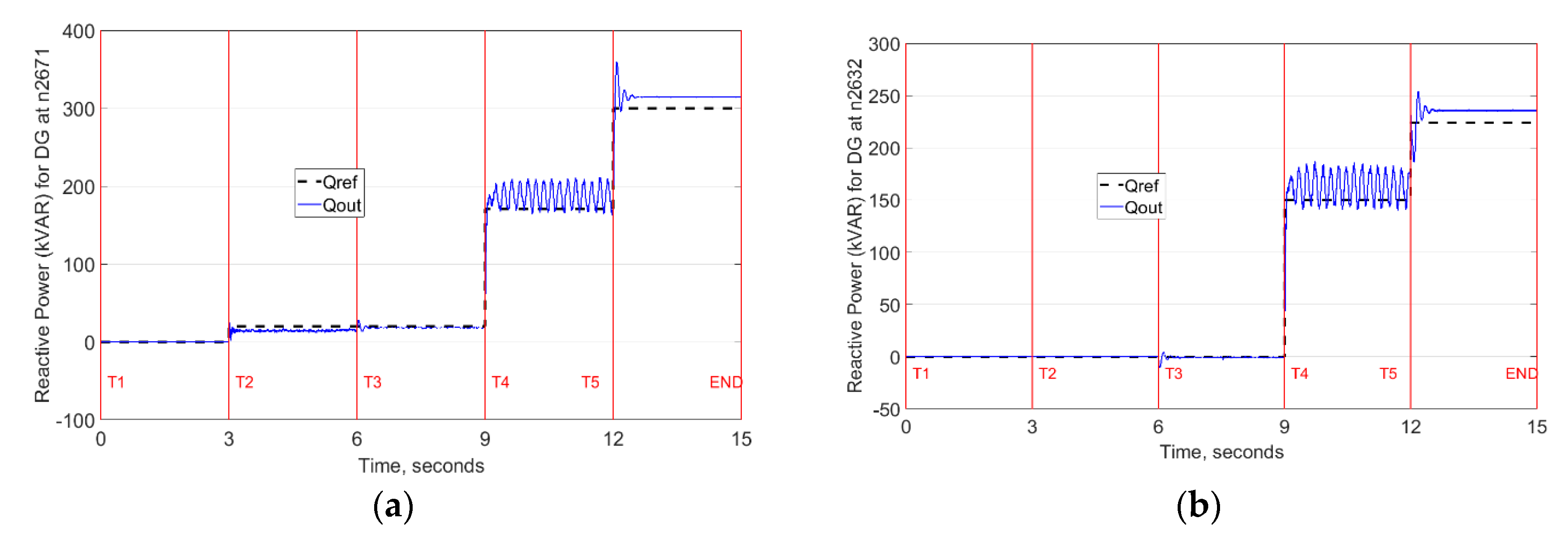
5.3. Solution Verification Using PSCAD Simulation as Benchmark

The restoration solution was set up for a time-domain simulation in PSCAD. Recall that in the power flow constraints section (Section 4.6), the power injection (output) for each droop DG has been set to be its reference active and reactive power. These ensure that each droop-controlled DG has an output voltage magnitude and frequency equal to its reference voltage and reference frequency, respectively, according to the droop equations. This, in turn, eliminates the droop co-efficient from its power injection expression since its output powers track their reference power setting.

It is more realistic that the reference powers of the droop-controlled DGs are not always accurately tracked, considering both physical and analytical concerns. Physical concerns are related to changing load profiles with time and power losses, which can lead to a power mismatch between the droop reference power settings and its output power. Analytical concerns are related to errors (such as linearization errors) in modeling the system, which could lead to power mismatch. Because of this power mismatch, the droop co-efficient plays a role in deciding how this mismatched power is shared among the droop-controlled DGs [43]. In addition, the droop coefficient plays a role in determining the stability of the system [44] and is thus an important parameter that affects the stable transition from one restoration step to the next. For the PSCAD simulation run in this section, the frequency droop coefficient was fixed to 0.0667 Hz per unit power and the voltage droop co-efficient was fixed to 0.00667 per unit power for all restoration steps. Both coefficients are expressed using the per phase power base of 1 MVA. The time interval between steps was fixed to 3 s. Determining threshold values for the droop coefficient settings and the time interval between any two adjacent steps for stable transition would be an interesting area for future work.

The metrics used for comparing results obtained from solving the restoration model with equivalent steady-state PSCAD results is the relative error. The relative error, ${\epsilon }_x$, of calculated quantity obtained from solving the restoration model, $x$, with respect to its reference PSCAD value (this PSCAD value is read when the transients have decayed/reached steady-state for each restoration step), $x_{ref}$, is defined as follows:

$${\epsilon }_x=\frac{\left|x-x_{ref}\right|}{\left|x_{ref}\right|}\times 100\%$$

(73)

The mean relative error, ${\overline{\epsilon }}_x$, of a set of calculated quantities is the mean of the relative errors of each element of the set.

Each component has been modeled with a detailed controller in PSCAD. Recall that the restoration solution was solved using a time step of 5. Assuming a time interval of 3 s between two adjacent time steps gives a total simulation time of 15 s. The PSCAD setup was run for a simulation time of 15 s. The power setpoint of the PQ DGs, droop reference power settings, load values and ZIP parameters, turn-on times for branches, loads, and DGs were set in the PSCAD according to the results obtained from the black start restoration solution of Section 5.2.

Figure 15 shows the droop reference active power for the two droop-controlled DGs. The red vertical lines are used to denote the time steps: T1, T2, etc. DG at node 2632 was synchronized to the microgrid at 6 s using the proposed zero-dispatch synchronization method. Notice that the synchronization is smooth. There is a sustained oscillation at the start of step 4. This sustained oscillation is mostly a function of the controller parameters. Readjusting these parameters to realize an exponentially stable step will involve detailed controller analysis and will be a focus for future study. By the start of step 5, the system became exponentially stable once again. Figure 15 shows that the droop DGs are able to track their reference active power setting across the restoration steps.

Figure 16 shows the droop frequency for the two droop-controlled DGs at nodes 2671 and 2632. Notice that they are regulated to approximately 60 Hz as desired. Furthermore, the DG at node 2632 has a pretty smooth synchronization to the microgrid at 6 s, which is the third restoration step.

Figure 17 shows the droop reference reactive power for the two droop-controlled DGs. Notice that there is a sustained oscillation at the start of step 4 just like in the active power and frequency plot of Figure 15 and Figure 16. This is because of the coupling between these parameters, as a sustained oscillation will manifest in several quantities at the same time. Just like in Figure 15, Figure 17 shows that the droop DGs are able to track their reference reactive power setting across the restoration steps.

The mean error of the nodal voltage magnitude across all nodes was calculated to be 1.40% when compared to the nodal voltages of the PSCAD simulation at the last restoration step. This means that on average the nodal voltage error of the restoration solution is in the order of ±0.014 per unit of the actual voltage magnitude. This mean error is further reduced to 0.058% by averaging out the unbalanced voltage effect due to filters and DGs’ controller response to unbalanced operation. This additional error due to filters and DGs’ controller response suggests that despite the system-wide unbalance compensation that the proposed restoration method handles, negative sequence compensation at the three-phase controlled DGs are necessary to improve voltage balance across all nodes in the microgrid.

6. Conclusions and Future Work

In this paper, a novel black start restoration formulation for an islanded microgrid was developed. The developed method enables the inter-connection of multiple droop-controlled master DGs to form the microgrid. The objective function was defined to maximize the total energy restored in the restoration steps of interest. Several operational constraints were identified and linearized to yield a mixed-integer linear programming (MILP) problem. Novel linear power flow constraints based on the current injection approach were formulated for an islanded droop-controlled microgrid without slack bus, and incorporated into the problem. The restoration method was used to solve for the restoration solution of an islanded microgrid adapted from the IEEE 13 node test feeder. Detailed PSCAD simulation was set up to verify the accuracy of the restoration solution. The PSCAD simulation shows that the DGs’ output power tracked their reference power, and suggests that despite load balancing constraints enforced by the restoration method, additional negative sequence compensation at the three-phase droop-controlled DGs is needed.

The number of restoration time steps influences the computational burden and size of the model. Increasing the number of time steps increases the model size and vice versa. Using a graph heuristic approach to determine the necessary number of steps to realize a better restoration solution will be considered in future work, and can help ensure that the model size is neither over-sized nor under-sized. Future work will also explore the use of the non-dispatchable DGs and loads with demand response, to enhance the restoration solution of the multi-master droop-controlled microgrids.

References

1. Hussain, A.; Bui, V.-H.; Kim, H.-M. Microgrids as a resilience resource and strategies used by microgrids for enhancing resilience. Appl. Energy 2019, 240, 56–72. [Google Scholar] [CrossRef]
2. Teimourzadeh, S.; Tor, O.B.; Cebeci, M.E.; Bara, A.; Oprea, S.V. A three-stage approach for resilience-constrained scheduling of networked microgrids. J. Mod. Power Syst. Clean Energy 2019, 7, 705–715. [Google Scholar] [CrossRef] [Green Version]
3. Cohn, L. California Microgrids Flex Their Skills During Blackouts. 2020. Available online: https://microgridknowledge.com/california-blackouts-microgrids-flexible-load/ (accessed on 15 September 2020).
4. Merchant, E.F. As Hurricane Season Approaches, More Microgrids Crop Up in Puerto Rico. Available online: https://www.greentechmedia.com/articles/read/as-hurricane-season-approaches-more-microgrids-cropping-up-in-puerto-rico (accessed on 4 June 2018).
5. Cohn, L. Microgrid Kept Power On Even as the California Wildfires Caused Outages. Available online: https://microgridknowledge.com/islanded-microgrid-fires/ (accessed on 29 November 2017).
6. Peters, A. New Microgrids Are Helping Australia Get Power Back after the Fires. Available online: https://www.fastcompany.com/90465605/new-microgrids-are-helping-australia-get-power-back-after-the-fires (accessed on 15 September 2020).
7. Farrokhabadi, M.; Cañizares, C.A.; Simpson-Porco, J.W.; Nasr, E.; Fan, L.; Mendoza-Araya, P.A.; Tonkoski, R.; Tamrakar, U.; Hatziargyriou, N.; Lagos, D.; et al. Microgrid Stability Definitions, Analysis, and Examples. IEEE Trans. Power Syst. 2020, 35, 13–29. [Google Scholar] [CrossRef]
8. Farrokhabadi, M.; König, S.; Cañizares, C.A.; Bhattacharya, K.; Leibfried, T. Battery Energy Storage System Models for Microgrid Stability Analysis and Dynamic Simulation. IEEE Trans. Power Syst. 2018, 33, 2301–2312. [Google Scholar] [CrossRef]
9. Chandorkar, M.C.; Divan, D.M.; Adapa, R. Control of parallel connected inverters in standalone AC supply systems. IEEE Trans. Ind. Appl. 1993, 29, 136–143. [Google Scholar] [CrossRef]
10. Rocabert, J.; Luna, A.; Blaabjerg, F.; Rodríguez, P. Control of Power Converters in AC Microgrids. IEEE Trans. Power Electron. 2012, 27, 4734–4749. [Google Scholar] [CrossRef]
11. Brabandere, K.D.; Bolsens, B.; Keybus, J.V.d.; Woyte, A.; Driesen, J.; Belmans, R. A Voltage and Frequency Droop Control Method for Parallel Inverters. IEEE Trans. Power Electron. 2007, 22, 1107–1115. [Google Scholar] [CrossRef]
12. Guo, W.; Mu, L. Control principles of micro-source inverters used in microgrid. Prot. Control Mod. Power Syst. 2016, 1, 5. [Google Scholar] [CrossRef]
13. Wang, Z.; Wang, J. Self-Healing Resilient Distribution Systems Based on Sectionalization Into Microgrids. IEEE Trans. Power Syst. 2015, 30, 3139–3149. [Google Scholar] [CrossRef]
14. Wang, Y.; Xu, Y.; He, J.; Liu, C.; Schneider, K.P.; Hong, M.; Ton, D.T. Coordinating Multiple Sources for Service Restoration to Enhance Resilience of Distribution Systems. IEEE Trans. Smart Grid 2019. [Google Scholar] [CrossRef] [Green Version]
15. Chen, C.; Wang, J.; Qiu, F.; Zhao, D. Resilient Distribution System by Microgrids Formation After Natural Disasters. IEEE Trans. Smart Grid 2016, 7, 958–966. [Google Scholar] [CrossRef]
16. Chen, B.; Chen, C.; Wang, J.; Butler-Purry, K.L. Sequential Service Restoration for Unbalanced Distribution Systems and Microgrids. IEEE Trans. Power Syst. 2018, 33, 1507–1520. [Google Scholar] [CrossRef]
17. Chen, B.; Chen, C.; Wang, J.; Butler-Purry, K.L. Multi-Time Step Service Restoration for Advanced Distribution Systems and Microgrids. IEEE Trans. Smart Grid 2018, 9, 6793–6805. [Google Scholar] [CrossRef]
18. Gilani, M.A.; Kazemi, A.; Ghasemi, M. Distribution system resilience enhancement by microgrid formation considering distributed energy resources. Energy 2020, 191, 116442. [Google Scholar] [CrossRef]
19. Fu, L.; Liu, B.; Meng, K.; Dong, Z.Y. Optimal Restoration of An Unbalanced Distribution System into Multiple Microgrids Considering Three-Phase Demand-Side Management. IEEE Trans. Power Syst. 2020. [Google Scholar] [CrossRef]
20. Lopes, J.A.P.; Moreira, C.L.; Madureira, A.G. Defining control strategies for MicroGrids islanded operation. IEEE Trans. Power Syst. 2006, 21, 916–924. [Google Scholar] [CrossRef] [Green Version]
21. Katiraei, F.; Iravani, M.R.; Lehn, P.W. Micro-grid autonomous operation during and subsequent to islanding process. IEEE Trans. Power Deliv. 2005, 20, 248–257. [Google Scholar] [CrossRef]
22. Che, L.; Khodayar, M.; Shahidehpour, M. Only Connect: Microgrids for Distribution System Restoration. IEEE Power Energy Mag. 2014, 12, 70–81. [Google Scholar] [CrossRef]
23. Nuschke, M. Development of a microgrid controller for black start procedure and islanding operation. In Proceedings of the 2017 IEEE 15th International Conference on Industrial Informatics (INDIN), Emden, Germany, 24–26 July 2017; pp. 439–444. [Google Scholar]
24. Vandoorn, T.L.; Vasquez, J.C.; Kooning, J.D.; Guerrero, J.M.; Vandevelde, L. Microgrids: Hierarchical Control and an Overview of the Control and Reserve Management Strategies. IEEE Ind. Electron. Mag. 2013, 7, 42–55. [Google Scholar] [CrossRef] [Green Version]
25. Kaur, A.; Kaushal, J.; Basak, P. A review on microgrid central controller. Renew. Sustain. Energy Rev. 2016, 55, 338–345. [Google Scholar] [CrossRef]
26. Bassey, O.; Butler-Purry, K.L.; Chen, B. Dynamic Modeling of Sequential Service Restoration in Islanded Single Master Microgrids. IEEE Trans. Power Syst. 2020, 35, 202–214. [Google Scholar] [CrossRef]
27. Simpson-Porco, J.W.; Dörfler, F.; Bullo, F. Droop-controlled inverters are Kuramoto oscillators. IFAC Proc. Vol. 2012, 45, 264–269. [Google Scholar] [CrossRef]
28. Saadat, H. Power System Analysis McGraw-Hill Series in Electrical Computer Engineering; Mcgraw-Hill College: New York, NY, USA, 1999. [Google Scholar]
29. Ahmadi, H.; Martı´, J.R.; von Meier, A. A Linear Power Flow Formulation for Three-Phase Distribution Systems. IEEE Trans. Power Syst. 2016, 31, 5012–5021. [Google Scholar] [CrossRef]
30. Williams, H.P. Model Building in Mathematical Programming; John Wiley & Sons: Hoboken, NJ, USA, 2013. [Google Scholar]
31. Bassey, O. Control and Black Start Restoration of Islanded Microgrids; Texas A&M University: College Station, TX, USA, 2020. [Google Scholar]
32. Renmu, H.; Ma, J.; Hill, D.J. Composite load modeling via measurement approach. IEEE Trans. Power Syst. 2006, 21, 663–672. [Google Scholar] [CrossRef]
33. IEEE Standard Test Procedure for Polyphase Induction Motors and Generators in IEEE Std 112-2017 (Revision of IEEE Std 112-2004); IEEE: New York, NY, USA, 2018; pp. 1–115.
34. Pillay, P.; Manyage, M. Definitions of voltage unbalance. IEEE Power Eng. Rev. 2001, 21, 50–51. [Google Scholar] [CrossRef]
35. Peng, L.; Bai, D.; Kang, Y.; Chen, J. Research on three-phase inverter with unbalanced load. In Proceedings of the Applied Power Electronics Conference and Exposition (APEC’04), Anaheim, CA, USA, 22–26 February 2004; Volume 121, pp. 128–133. [Google Scholar]
36. Bassey, O.; Butler-Purry, K.L. Modeling Single-Phase PQ Inverter for Unbalanced Power Dispatch in Islanded Microgrid. In Proceedings of the 2019 IEEE Texas Power and Energy Conference (TPEC), College Station, TX, USA, 7–8 February 2019; pp. 1–6. [Google Scholar]
37. Adibi, M.; Clelland, P.; Fink, L.; Happ, H.; Kafka, R.; Raine, J.; Scheurer, D.; Trefny, F. Power System Restoration—A Task Force Report. IEEE Trans. Power Syst. 1987, 2, 271–277. [Google Scholar] [CrossRef]
38. Lavorato, M.; Franco, J.F.; Rider, M.J.; Romero, R. Imposing Radiality Constraints in Distribution System Optimization Problems. IEEE Trans. Power Syst. 2012, 27, 172–180. [Google Scholar] [CrossRef]
39. Lofberg, J. YALMIP: A toolbox for modeling and optimization in MATLAB. In Proceedings of the 2004 IEEE International Conference on Robotics and Automation (IEEE Cat. No.04CH37508), New Orleans, LA, USA, 2–4 September 2004; pp. 284–289. [Google Scholar]
40. Gurobi Optimization. Available online: http://www.gurobi.com/ (accessed on 15 September 2020).
41. Baran, M.E.; Wu, F.F. Network reconfiguration in distribution systems for loss reduction and load balancing. IEEE Trans. Power Deliv. 1989, 4, 1401–1407. [Google Scholar] [CrossRef]
42. Gan, L.; Low, S.H. Convex relaxations and linear approximation for optimal power flow in multiphase radial networks. In Proceedings of the 2014 Power Systems Computation Conference, Wroclaw, Poland, 18–22 August 2014; pp. 1–9. [Google Scholar]
43. Bassey, O.; Butler-Purry, K.L.; Chen, B. Active and Reactive Power Sharing in Inverter Based Droop-Controlled Microgrids. In Proceedings of the 2019 IEEE Power & Energy Society General Meeting (PESGM), Atlanta, GA, USA, 4–8 August 2019; pp. 1–5. [Google Scholar]
44. Barklund, E.; Pogaku, N.; Prodanovic, M.; Hernandez-Aramburo, C.; Green, T.C. Energy Management in Autonomous Microgrid Using Stability-Constrained Droop Control of Inverters. IEEE Trans. Power Electron. 2008, 23, 2346–2352. [Google Scholar] [CrossRef] [Green Version]
Figure 1. Droop graph for (a) frequency droop (b) voltage droop, with reference/desired operation points.
Energies 13 05996 g001
Figure 2. Islanded microgrid representation with loads, droop controlled distributed generators (DGs) and PQ DGs.
Energies 13 05996 g002
Figure 3. 14-Node distribution system waiting to be restored.
Energies 13 05996 g003
Figure 4. Step 1, 2, and 3 of an Example Restoration Process.
Energies 13 05996 g004
Figure 5. (a) Step 4 and (b) Step 5 of the Example Restoration Process.
Energies 13 05996 g005
Figure 6. Parallel restoration with master DG and problem with synchronization and interconnecting the restored microgrids.
Energies 13 05996 g006
Figure 7. Flowchart of the proposed restoration method.
Energies 13 05996 g007
Figure 8. Three-node example to illustrate power flow constraints for droop-controlled microgrids.
Energies 13 05996 g008
Figure 9. Illustration of bus block reduction using Modified IEEE 13 node test feeder.
Energies 13 05996 g009
Figure 10. One-line diagram of modified IEEE 13 node test feeder.
Energies 13 05996 g010
Figure 11. Restoration Sequence Result, with (ae) representing step 1, 2, to 5 respectively.
Energies 13 05996 g011
Figure 12. (a) Droop three-phase active power reference (b) Droop three-phase reactive power reference.
Energies 13 05996 g012
Figure 13. (a) PQ DG active power setpoint (b) PQ DG reactive power setpoint.
Energies 13 05996 g013
Figure 14. Voltage magnitude across all nodes at the last restoration step.
Energies 13 05996 g014
Figure 15. Droop reference active power and output active power for DGs at nodes (a) 2671 and (b) 2632 as obtained from PSCAD simulation.
Energies 13 05996 g015
Figure 16. Droop frequency for DGs at nodes 2671 and 2632 as obtained from PSCAD simulation.
Energies 13 05996 g016
Figure 17. Droop reference reactive power and output reactive power for DGs at nodes (a) 2671 and (b) 2632 as obtained from PSCAD simulation.
Energies 13 05996 g017