Early Fault Detection of Gas Turbine Hot Components Based on Exhaust Gas Temperature Profile Continuous Distribution Estimation

Abstract

Failures of the gas turbine hot components often cause catastrophic consequences. Early fault detection can detect the sign of fault occurrence at an early stage, improve availability and prevent serious incidents of the plant. Monitoring the variation of exhaust gas temperature (EGT) is an effective early fault detection method. Thus, a new gas turbine hot components early fault detection method is developed in this paper. By introducing a priori knowledge and quantum particle swarm optimization (QPSO), the exhaust gas temperature profile continuous distribution model is established with finite EGT measuring data. The method eliminates influences of operating and ambient condition changes and especially the gas swirl effect. The experiment reveals the presented method has higher fault detection sensitivity.

1. Introduction

The hot components are the crucial components of gas turbines, including the combustors and turbines. A higher gas temperature at the outlet of the combustors brings higher efficiency to the gas turbine but also brings higher potential safety hazards to the gas turbine hot components. The hot components failures often cause serious incidents and huge economic losses. Early fault detection is a particularly significant way to improve the availability and reliability of hot components.

Exhaust gas temperature (EGT) is usually used as an indicator to detect the fault in the gas turbine hot components. Several thermocouples with uniform distribution at the turbine exhaust section are used to measure the EGT. The healthy hot components cause a uniform EGT profile, whereas the hot component faults could cause the uneven EGT profile. Therefore, some indicators which describe the uniformity of the EGT profile are presented. The system [1] produced by GE monitors the variance of EGT values about the mean. An increasing temperature variance usually indicates a hot component malfunction. The MARK VI system [2], another monitor system produced by GE and as one of the most widely used system, utilizes temperature differences between the maximum and the three minimum EGT values. It defines a parameter, allowable exhaust temperature dispersion, which is a function of the average EGT and the compressor outlet temperature. The higher the ratio of the temperature differences to the allowable exhaust temperature dispersion, the greater the possibility of fault. Gulen et al. [3] introduced a heavy-duty industrial gas turbine real-time online performance diagnostic system. In the system, excessive and sudden changes or consistent upward trends in the ratio of the maximum EGT to the average of EGT indicate the potential combustor faults. However, in practical operation, these methods are not sensitive to fault signals. When the detection system alarms, the components have been seriously damaged [4].

The temperature differences between different EGT values could be caused not only by the hot component faults but also by various ambient and operating conditions. It sometimes has a greater influence on EGT than the faults. Therefore, it is hard to identify the faults from the interference. The above methods cannot achieve satisfactory sensitivity simply by monitoring the temperature differences.

Several EGT models are presented, and the abnormalities are detected by high residuals between actual and estimated EGT values. Yılmaz [5] and Song et al. [6] present two multiply linear regression EGT models using different operating parameters, respectively. Tarassenko et al. [7] build an EGT model based on artificial neural networks (ANN), and ANN is used to learn the relationship between various EGTs. Yan [8] presents a data-driven EGT model based on deep learning and proposed a deep semi-supervised anomaly detection (deepSSAD). Basseville et al. [9,10] describe an EGT physical model and detect the changes in the coefficient of the model. Based on the simple Brayton cycle, Medina et al. [11] propose an EGT model that considered the rotation of hot gas in turbines. Liu et al. [12] present an indicator that characterizes the intrinsic structure information of hot components and describes the relationship between the EGT value and the average of all the EGT values. Talaat et al. [13] established a thermodynamic model to simulate gas turbine performance and proposed a diagnosis system based on ANN to detect the deterioration of engine performance. Chen [14] used a data mining algorithm based on radial basis function (RBF) neural networks to predict the EGT. Pi et al. [15] proposed the improved quantum-behaved particle swarm optimization support vector regression model to predict EGT. It can be found that the establishment of the EGT model is developing from a mechanism model based on the thermodynamic cycle to a data-driven model combined with a large number of algorithms. The EGT model proposed in this paper is based on the integration of gas turbine prior knowledge and intelligent algorithm and possesses a more reasonable model structure. The influence of different ambient and operating conditions on EGT includes two aspects. The first one is the EGT profile scaling with the ambient and operating conditions. With the change of ambient and operating conditions, every EGT value increases and decreases simultaneously. Moreover, the air and fuel mix at a high temperature in the combustor, and then the hot gas drives the turbine to spin and rotates with the turbine blades. Hence, there is a swirl angle between the combustor and the exhaust thermocouple measuring the temperature of the hot gas from this combustor. The swirl angle changes with the ambient and operating conditions. Hence, the second aspect is the EGT profile swirl with the ambient and operating conditions. However, most previous work focus on the scaling effect and few studies consider the swirl effect. In the EGT model presented by Basseville et al. [9,10], the swirl angle is considered and calculated by the physical principles. However, it is based on some hypotheses, and some details of the gas turbine need to be known, for example, the size of the gas turbine.

To improve detecting sensitivity, the influence of different ambient and operating conditions on the EGT profile should be fully considered, especially the swirl effect. Actually, before and after the ambient or operating conditions change, one exhaust thermocouple measuring results may reveal the performance of different combustor because of the swirl effect. However, there exists an intrinsic relationship between the thermocouple measuring points, so a continuous circumferential EGT profile distribution model can be developed with finite EGT measuring data, and accurate EGT evaluation under the swirl effect can be obtained.

Based on the characteristics of the EGT profile, a novel early fault detection method of gas turbine hot components is developed. The developed method fully considers the influence of different ambient and operating conditions on the EGT profile by estimating the EGT profile’s continuous distribution.

The remainder of this paper is organized as follows: The second section proposes an early fault detection method based on continuous EGT distribution evaluation. The third section verifies the availability of the proposed method with experiments, follows, which is the conclusion.

2. Early Fault Detection Method

2.1. Influence of Gas Rotation on EGT Profile

The temperature at the exit of the combustion chamber is so high that the conventional thermocouple cannot work in such an environment for a long time. Therefore, the EGT, which is measured by several thermocouples evenly distributed at the turbine outlet, is widely used to indirectly monitor the performance of hot components. The distribution of the combustion chamber and thermocouple of a gas turbine is shown in Figure 1. Ideally, the structure of each combustor is basically identical, and the temperature measured by each thermocouple is basically the same. However, when a combustor faults, its outlet temperature will be affected, which shows local high temperature or local low temperature. This abnormal signal will be transmitted to thermocouples, and the corresponding thermocouple’s reading is going to be different from others. Therefore, when the gas turbine is operating normally, the EGT profile is uniform, and when the EGT profile is locally uneven, it indicates that the hot components have faulted, as shown in Figure 2. The greater the temperature discrepancy between different thermocouple readings, the greater the possibility of hot component faults.

Operating and ambient conditions also cause temperature discrepancies. In previous work [12], the EGT profile scaling under different operating and ambient conditions are mainly discussed. The EGT profile also swirls under different operating and ambient conditions with the rotation of the turbine, as described in Figure 3. As a result, the gas temperature measured by the thermocouple is not from the combustor at the same angular position. There is a swirl angle, which depends on the operating and ambient conditions, between the combustor and the thermocouple measuring the temperature of the hot gas from this combustor. As depicted in Figure 4, the position of the thermocouples is fixed, and the EGT profile swirls under different operating and ambient conditions. It can be seen that the change of the swirl angle may cause the temperature discrepancies between different thermocouple readings to change.

As described above, temperature discrepancies can be caused by either hot components fault or operating and ambient change. Therefore, in actual applications, in order to reduce the false alarm rate, the fault detection threshold is generally set larger. This also leads to a high missing alarm rate, which reduces the sensitivity of detection and makes faults unable to be detected as early as possible. Therefore, the influences of operating and ambient condition change, and especially the swirl effect, should be eliminated in gas turbine hot components early fault detection.

2.2. EGT Profile Continuous Distribution Estimation

2.2.1. EGT Profile Model

Hot gas from different combustors mix and rotate in the turbine; therefore, the reading of a certain EGT thermocouple is affected by gas from more than one combustor. Suppose the influence of a combustor on EGT thermocouple reading presents normal distribution, and the influence scope of each combustor is the same. Then according to Ref. [11], the EGT distribution can be described as:

$$T_{4,i}=\mathrm{A}·{{\displaystyle \sum }}_{j=1}^n{T}_{4c}^j·\frac{1}{\sqrt{2\pi }\sigma }\exp \left(-{\left(\frac{{\mathsf{\Phi }}_i^t-{\mathsf{\Phi }}_j^c}{\sigma }\right)}^2\right)$$

(1)

where $T_{4,i}$ is the i-th thermocouple EGT reading, $T_{4c}^j$ is the j-th turbine channel (namely, the turbine at the same angle with the j-th combustor) outlet temperature, n is the number of combustor and turbine channel. ${\mathsf{\Phi }}_i^t$ is the position of the i-th thermocouple, ${\mathsf{\Phi }}_j^c$ is the position of the j-th combustor, and $\sigma$ is the variance of the normal distribution, which reflects each combustor’s influence scope on exhaust temperature. $\sigma$ is determined by experience; a larger $\sigma$ value represents a larger influence scope and vice versa.

It should be noticed that $T_{4c}^j$ does not actually exist, it is an imaginary j-th EGT value when no swirl happens, and it can be calculated by turbine average outlet temperature:

$$T_{4c}^j={\theta }_j{T}_{4,avg}$$

(2)

Then

$$T_{4,i}=\mathrm{A}·{{\displaystyle \sum }}_{j=1}^n{\theta }_j{T}_{4,avg}·\frac{1}{\sqrt{2\pi }\sigma }\exp \left(-{\left(\frac{{\mathsf{\Phi }}_i^t-{\mathsf{\Phi }}_j^c}{\sigma }\right)}^2\right)$$

(3)

Suppose that gas swirl angle is D and exhaust temperature can be written as the following:

$$T_{4,i}=\mathrm{A}·{{\displaystyle \sum }}_{j=1}^n{\theta }_j{T}_{4,avg}·\frac{1}{\sqrt{2\pi }\sigma }\exp \left(-{\left(\frac{{\mathsf{\Phi }}_i^t-{\mathsf{\Phi }}_j^c-D}{\sigma }\right)}^2\right)$$

(4)

Gas flow character in the turbine rotor and stator can be calculated with the method raised by Zhang [16]. However, considering the complexity of this method, in this paper, the swirl angle is obtained by multiple linear regression fitting with average EGT, compressor outlet pressure and ambient temperature, as:

$$D=a{T}_{4,avg}+b{P}_2+c{T}_1+d$$

(5)

where $T_{4,avg}$ is turbine average exhaust temperature, $P_2$ is compressor outlet pressure, and $T_1$ is ambient temperature. As shown in Figure 5 and Figure 6, the swirl angle is well fitted.

Then Equation (4) can be rewritten as the following:

$$T_{4,i}=\mathrm{A}·{{\displaystyle \sum }}_{j=1}^n\left({\theta }_j{T}_{4,avg}\right)·\frac{1}{\sqrt{2\pi }\sigma }\exp \left(-{\left(\frac{{\mathsf{\Phi }}_i^t-{\mathsf{\Phi }}_j^c-\left(a{T}_{4,avg}+b{P}_2+c{T}_1+d\right)}{\sigma }\right)}^2\right)$$

(6)

Of all the parameters in Equation (6), $\mathrm{A}$ and $\sigma$ characterize the influence scope of every combustor and can be decided by experience. If $\left({\theta }_j,a,b,c,d\right)$ can be estimated, the EGT profile continuous distribution can be determined.

In this paper, a priori knowledge is introduced to establish the EGT profile model. The model reveals the relationship between EGT thermocouple readings, and the effect of gas swirl angle is considered. With this model, continuous circumferential EGT distribution at any moment can be determined with finite EGT measuring data.

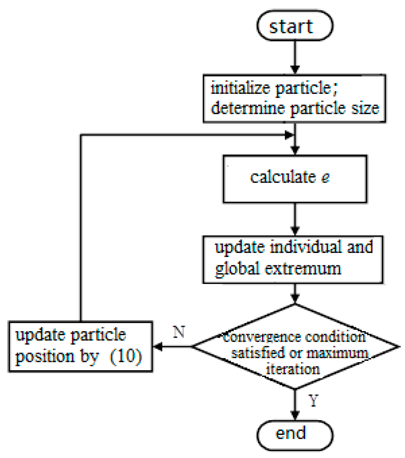
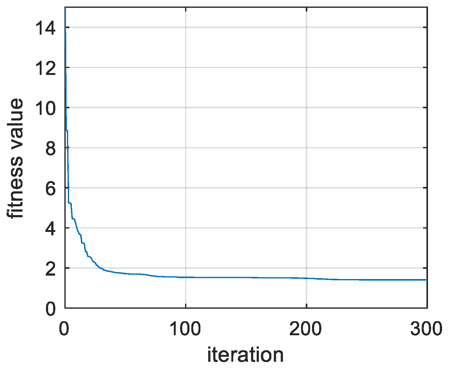
2.2.2. Parameter Evaluation

In this part, the quantum particle swarm optimization (QPSO) method [17] is introduced to estimate parameter $\left({\theta }_j,a,b,c,d\right)$ from Equation (6). QPSO method decides a group of random particles (namely, random solutions) as the initial value. Through continuous iteration, each particle updates to the optimal solution by following the current optimal particle. QPSO method updates particle position as following:

$$P_{ij}^t=\left({\phi }_1{p}_{ij}^t+{\phi }_2{p}_{gj}^t\right)/\left({\phi }_1+{\phi }_2\right)$$

(7)

$$mbest=\frac{1}{M}{\displaystyle \sum }_{i=1}^M{p}_i$$

(8)

$$b=1-0.5\times \frac{t}{maxgeneration}$$

(9)

$$x_{ij}^{t+1}=P_{ij}^t\pm \alpha \left|mbest-x_{ij}^t\right|\times ln\frac{1}{u}$$

(10)

where $mbest$ is the middle position of $p_i$, the individual optimum position of M particles. $b$ is contraction factor, $t$ is the current number of generation, and $maxgeneration$ is the maximum number of generations. $\alpha$ and $u$ are random numbers from (0,1). When u < 0.5, the operation ‘$\pm$’ in function (10) is ‘−’.

To find the parameters that minimize the deviation between exhaust gas temperature and model output result, the fitness function is defined as:

$$e=\sqrt{\frac{1}{m}{{\displaystyle \sum }}_{i=1}^m{\left({\widehat{T}}_{4,i}-T_{4,i}\right)}^2}$$

(11)

$${\widehat{T}}_{4,i}={{\displaystyle \sum }}_{j=1}^n\left({\widehat{\theta }}_j{T}_{4,avg}\right)·\frac{1}{\sqrt{2\pi }\sigma }\exp \left(-{\left(\frac{{\mathsf{\Phi }}_i^t-{\mathsf{\Phi }}_j^c-\left(\widehat{a}{T}_{4,avg}+\widehat{b}{P}_2+\widehat{c}{T}_1+\widehat{d}\right)}{\sigma }\right)}^2\right)$$

(12)

The parameter process of the QPSO method evaluation model is shown in Figure 7. First, the parameter set $\left({\theta }_j,a,b,c,d\right)$ is initialized with random particles. We substitute the particles into Equation (11) to calculate a fit value e and update the individual and global extrema of the group. If e satisfies the convergence condition or the number of iterations reaches the maximum, we stop the iteration. Else, we update the particle position by Equation (10). Moreover, the final position of the particles is the parameter set to evaluate.

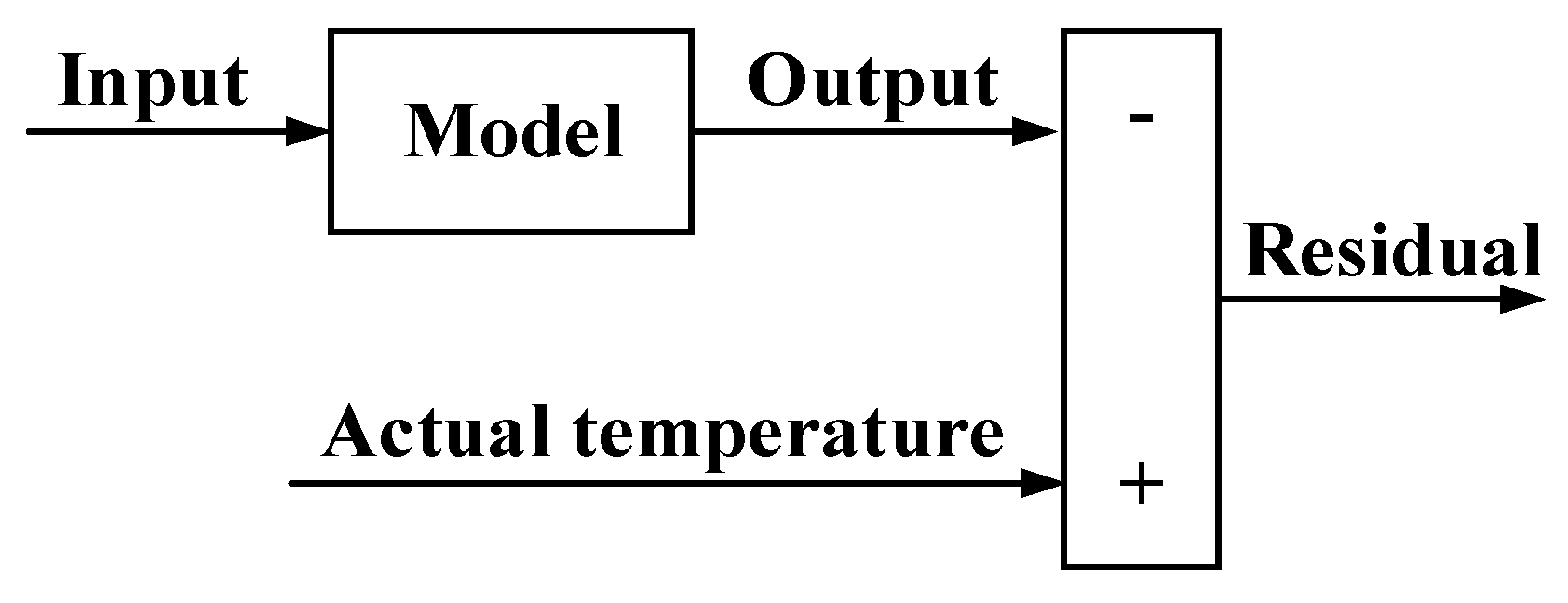
2.3. Gas Turbine Hot Components Early Fault Detection

The EGT profile continuous distribution estimation method proposed in this paper takes a priori knowledge into consideration and enables estimating gas turbine continuous circumferential EGT distribution with finite measuring data. Therefore, the thermocouple readings can be accurately evaluated when gas swirl happens.

The early fault detection method based on the proposed EGT distribution model is shown in Figure 8. The parameters are evaluated with gas turbine normal operation data, and the output of the model is estimated thermocouple reading. If the gas turbine is healthy, the estimated thermocouple reading and actual thermocouple reading are almost the same, and the residual will be stable. In contrast, if there is something wrong with the hot components, the estimated thermocouple reading and actual thermocouple reading are totally different, and the residual will increase.

3. Experiments

In this section, the sensitivity of the developed method is evaluated. The training dataset is simulated by the gas turbine model from [16,18]. Exhaust temperature and swirl angle during this time period is shown in Figure 9 and Figure 10. The tested gas turbine has 6 combustors and 31 EGT thermocouple measuring points. The model proposed in this paper is compared with a multiple linear regression model proposed in [12]. The multiple linear regression model is an EGT evaluation model with average exhaust temperature, compressor outlet pressure and ambient temperature, but the model does not take the influence of gas swirl into account.

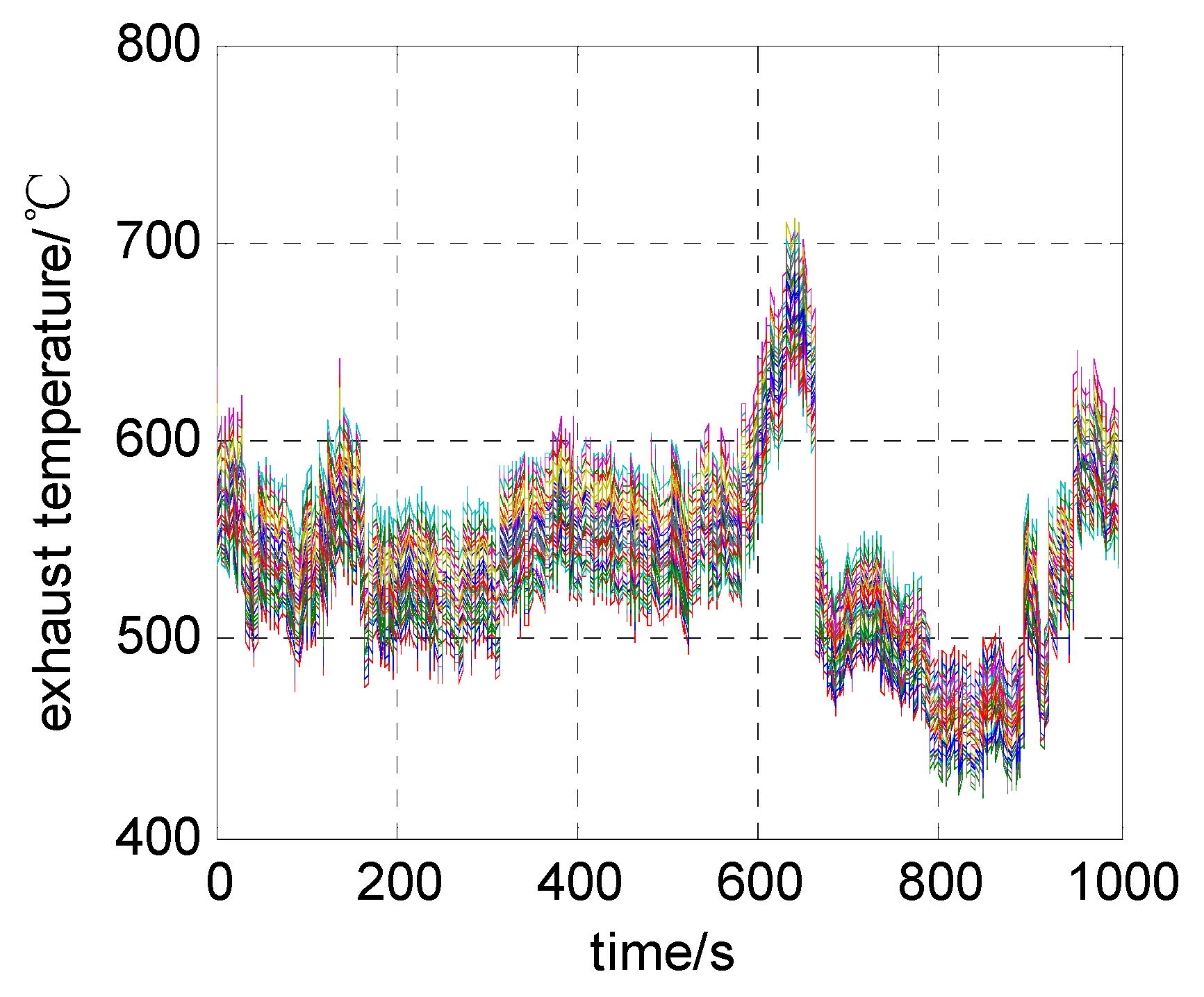
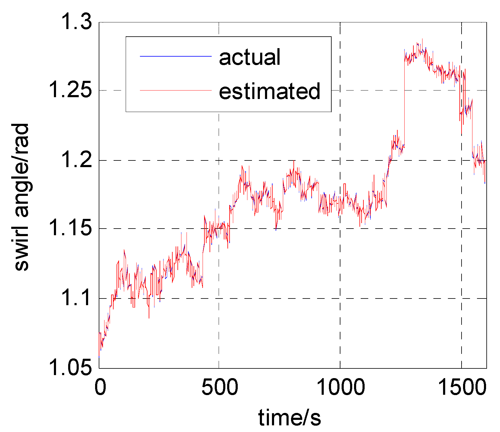
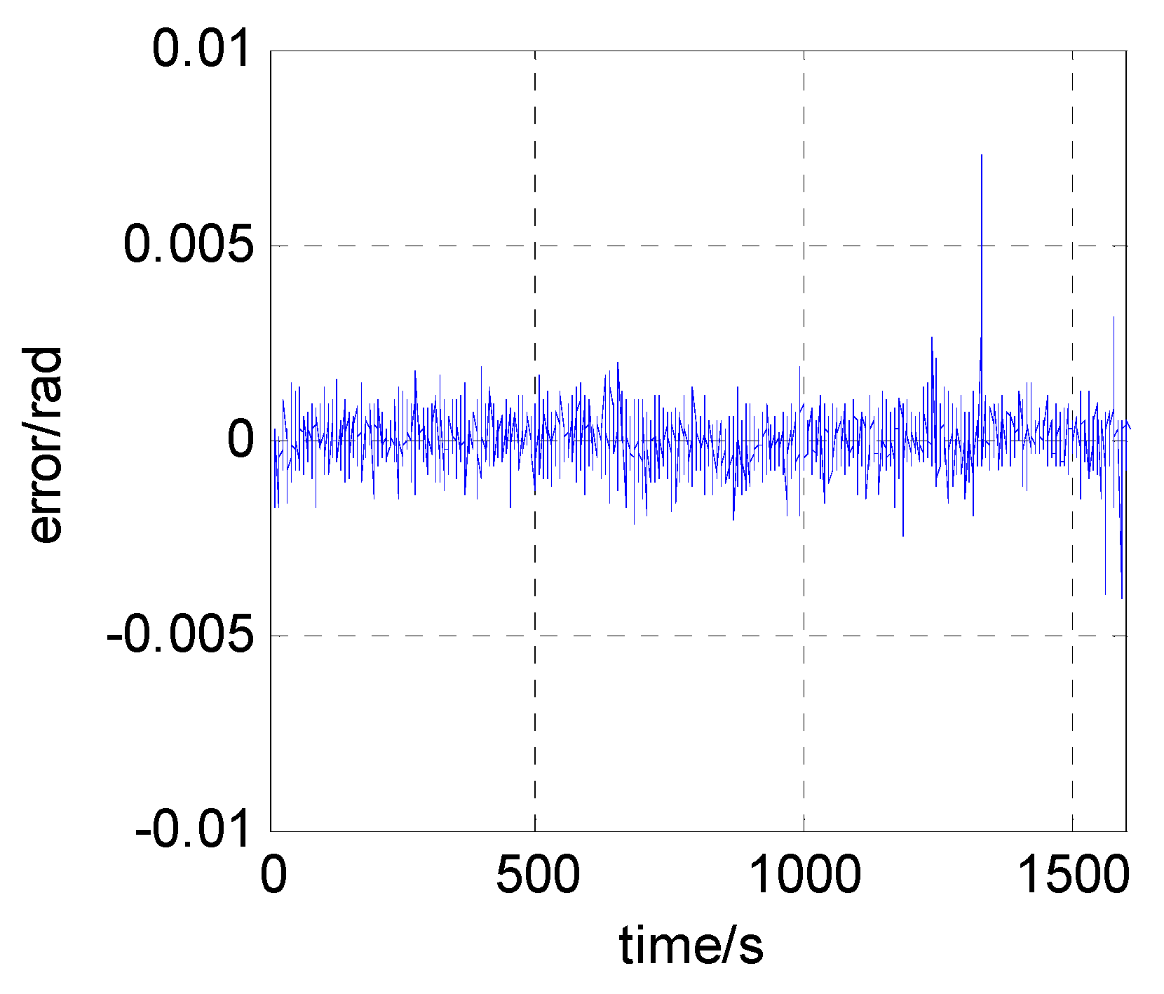
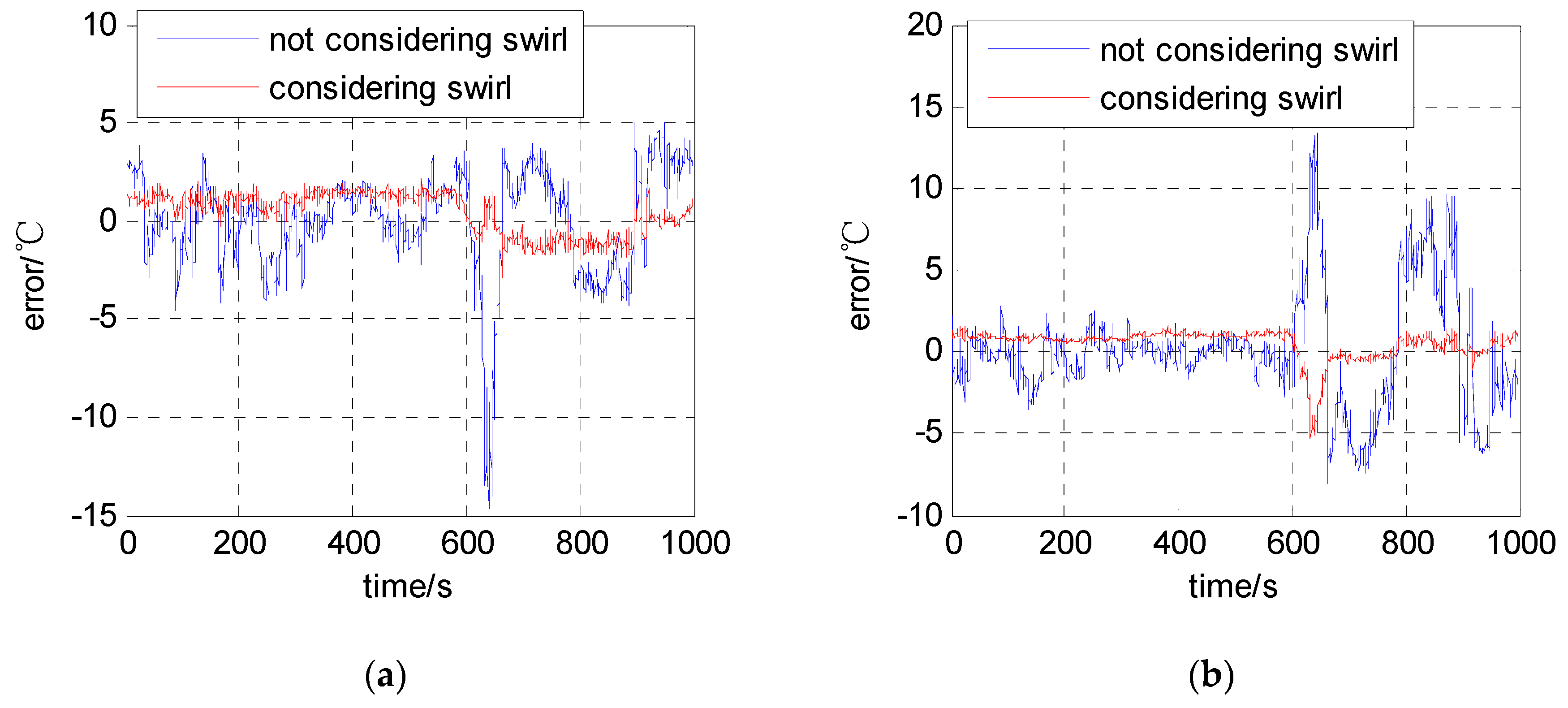
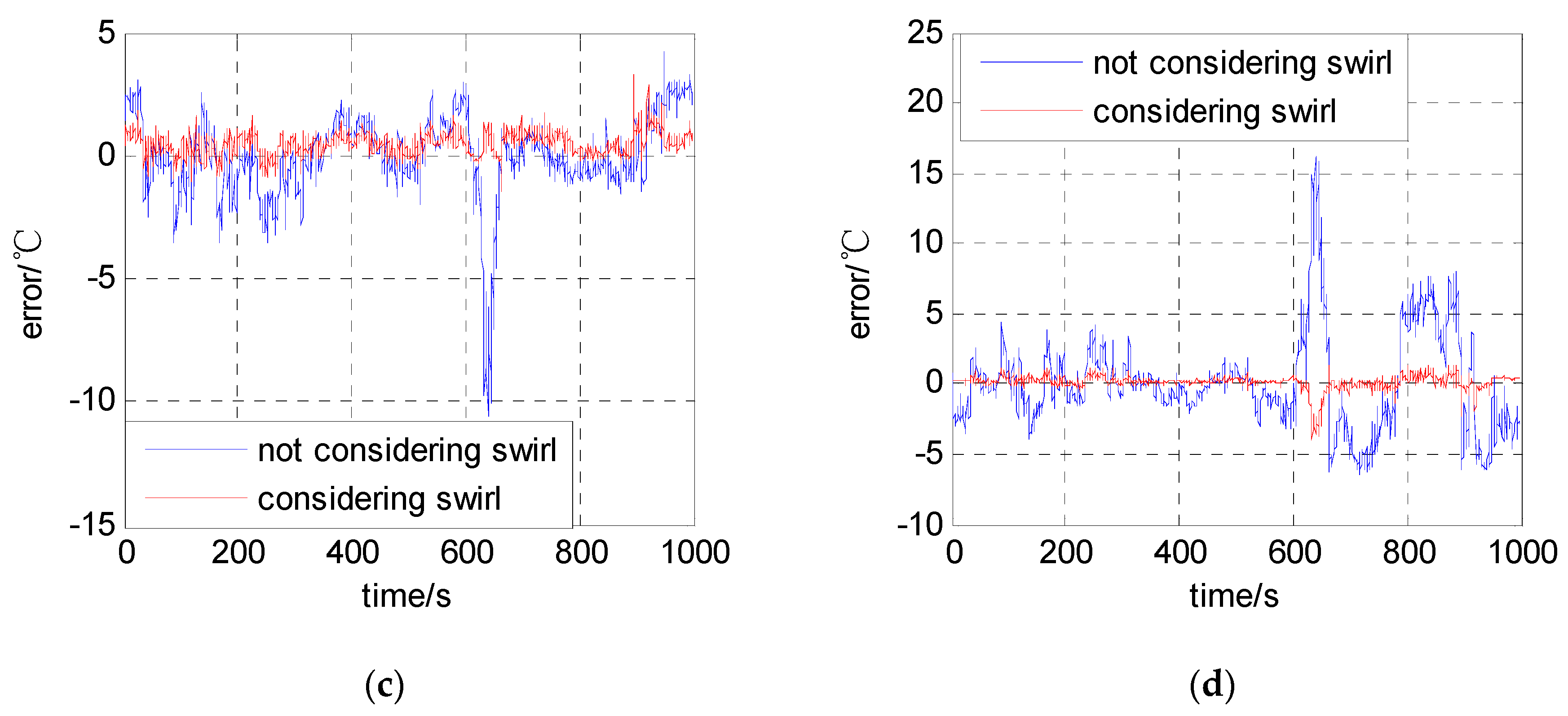
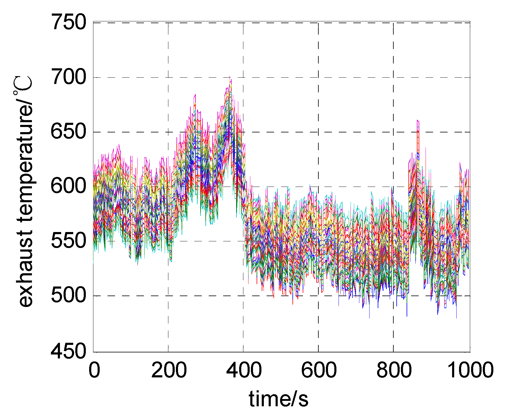
3.1. EGT Profile Estimation Result

First, parameter $\left({\theta }_j,a,b,c,d\right)$ is evaluated with data from 31 EGT measuring points. The parameter process of the QPSO method-based evaluation model is shown in Figure 7, and the initialization parameters are shown in

Table 1. Initialization parameters of the QPSO method.

Parameters	Initial Value
${\theta }_j$	$\left[0.9,1.1\right]$
a	$\left[-1,0\right]$
b	$\left[-1,0\right]$
c	$\left[-1,0\right]$
d	$\left[0,2\right]$
Number of evolutions	300
Particle group size	300

.

The fitness function of QPSO is calculated by Equation (11). It guarantees that the parameter set minimizes the deviation between actual exhaust temperature and model result. The QPSO method optimal curve is shown in Figure 11. After 300 iterations, the fitness value is small and stable enough, and the error is acceptable. The parameter evaluation result is shown in

Table 2. Parameter evaluation result.

Parameters	Value	Parameters	Value
${\theta }_1$	1.006	${\theta }_6$	0.987
${\theta }_2$	0.977	a	−0.318
${\theta }_3$	0.994	b	−0.397
${\theta }_4$	1.022	c	−0.254
${\theta }_5$	1.012	b	1.497

. Moreover, he obtained parameters can be used in Equation (6).

The error of evaluation between models proposed in this paper (considering the swirl effect) and that proposed in reference [12] (not considering swirl effect) is shown in Figure 12. It is obvious that when a gas swirl happens, the model not considering the swirl effect has a larger error value. Define the maximum and minimum residuals between the actual values and the model output values of each measuring point as threshold values for early fault detection; this is shown in

Table 3. Threshold values of two detection methods.

Measuring Point NO.	Not Considering Swirl Effect		Considering Swirl Effect		Measuring Point NO.	Not Considering Swirl Effect		Considering Swirl Effect
	Upper Limit /°C	Lower Limit /°C	Upper Limit/°C	Lower Limit/°C		Upper Limit /°C	Lower Limit /°C	Upper Limit /°C	Lower Limit /°C
$T_{4,1}$	12.74	−6.95	1.86	−5.40	$T_{4,17}$	14.49	−5.10	2.82	−2.08
$T_{4,2}$	5.55	−3.84	2.45	−4.35	$T_{4,18}$	5.92	−9.43	3.76	−2.43
$T_{4,3}$	6.92	−10.77	2.10	−2.75	$T_{4,19}$	8.13	−14.24	5.65	−2.02
$T_{4,4}$	5.03	−14.63	2.12	−2.83	$T_{4,20}$	3.83	−9.32	2.40	−2.26
$T_{4,5}$	8.68	−5.37	2.60	−3.46	$T_{4,21}$	9.99	−6.88	1.51	−3.20
$T_{4,6}$	13.34	−8.11	1.58	−5.31	$T_{4,22}$	12.91	−5.05	1.50	−4.13
$T_{4,7}$	8.97	−3.71	1.51	−2.50	$T_{4,23}$	3.74	−7.47	1.89	−2.64
$T_{4,8}$	6.57	−10.37	2.84	−1.27	$T_{4,24}$	7.20	−13.85	3.16	−1.19
$T_{4,9}$	5.72	−14.52	4.25	−2.27	$T_{4,25}$	4.23	−10.61	3.25	−1.52
$T_{4,10}$	7.72	−4.04	4.18	−3.14	$T_{4,26}$	11.17	−7.33	2.75	−3.02
$T_{4,11}$	14.64	−8.29	3.81	−4.00	$T_{4,27}$	16.20	−6.53	1.41	−3.84
$T_{4,12}$	13.93	−4.93	3.98	−3.42	$T_{4,28}$	5.76	−5.75	3.05	−3.20
$T_{4,13}$	7.01	−10.46	4.16	−3.35	$T_{4,29}$	8.38	−11.29	4.72	−2.90
$T_{4,14}$	7.44	−14.22	5.92	−2.29	$T_{4,30}$	4.64	−13.25	3.39	−3.43
$T_{4,15}$	4.51	−5.43	3.65	−2.37	$T_{4,31}$	8.71	−5.26	2.18	−4.06
$T_{4,16}$	11.53	−7.28	2.45	−2.48

. The model proposed in this paper reduces the influence of gas swirl effectively, compresses fault detection threshold, and increases fault detection sensitivity.

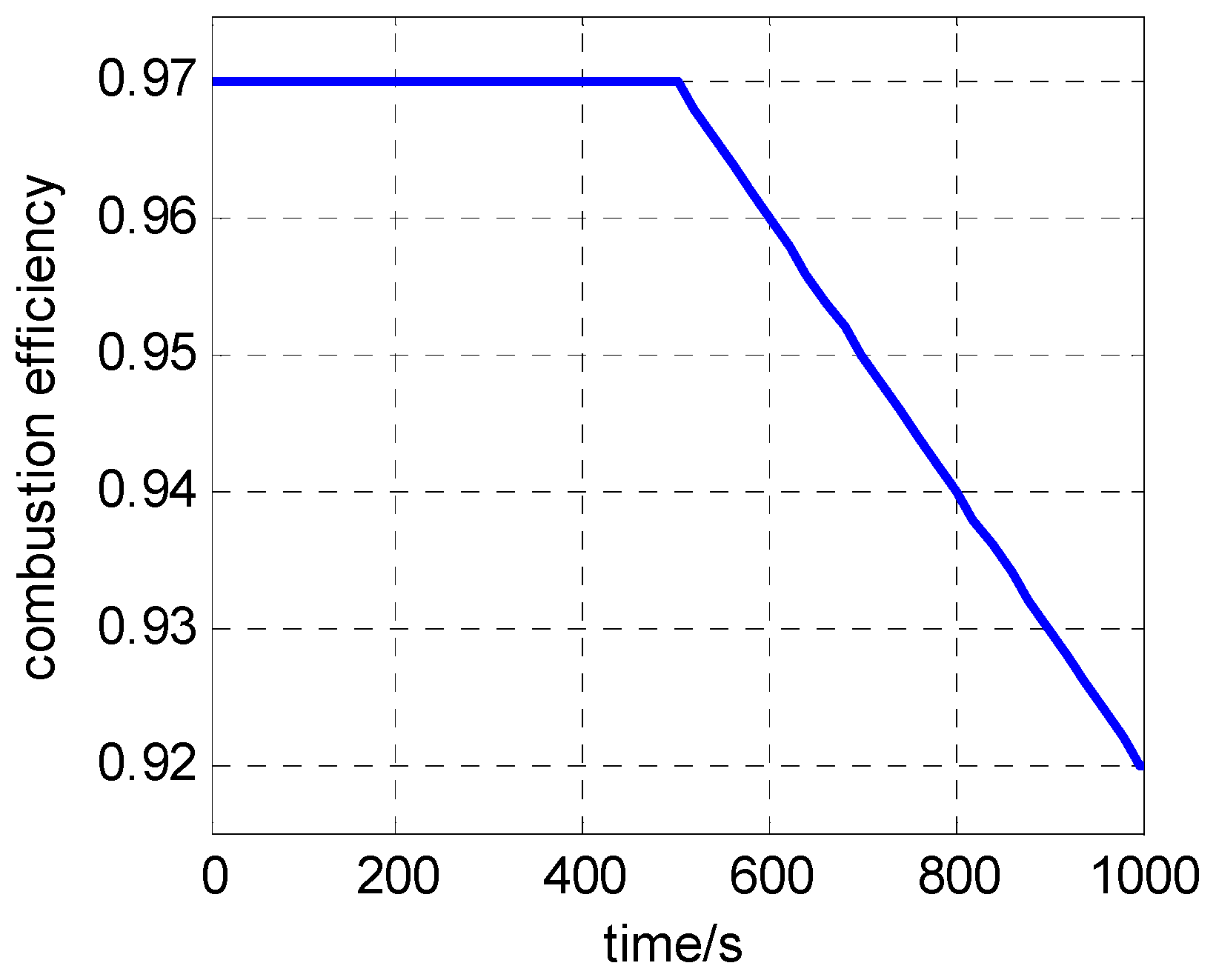
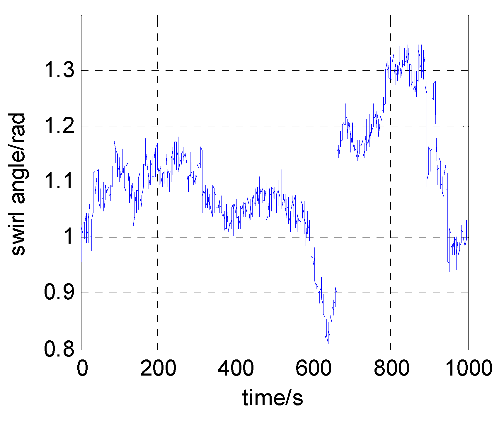
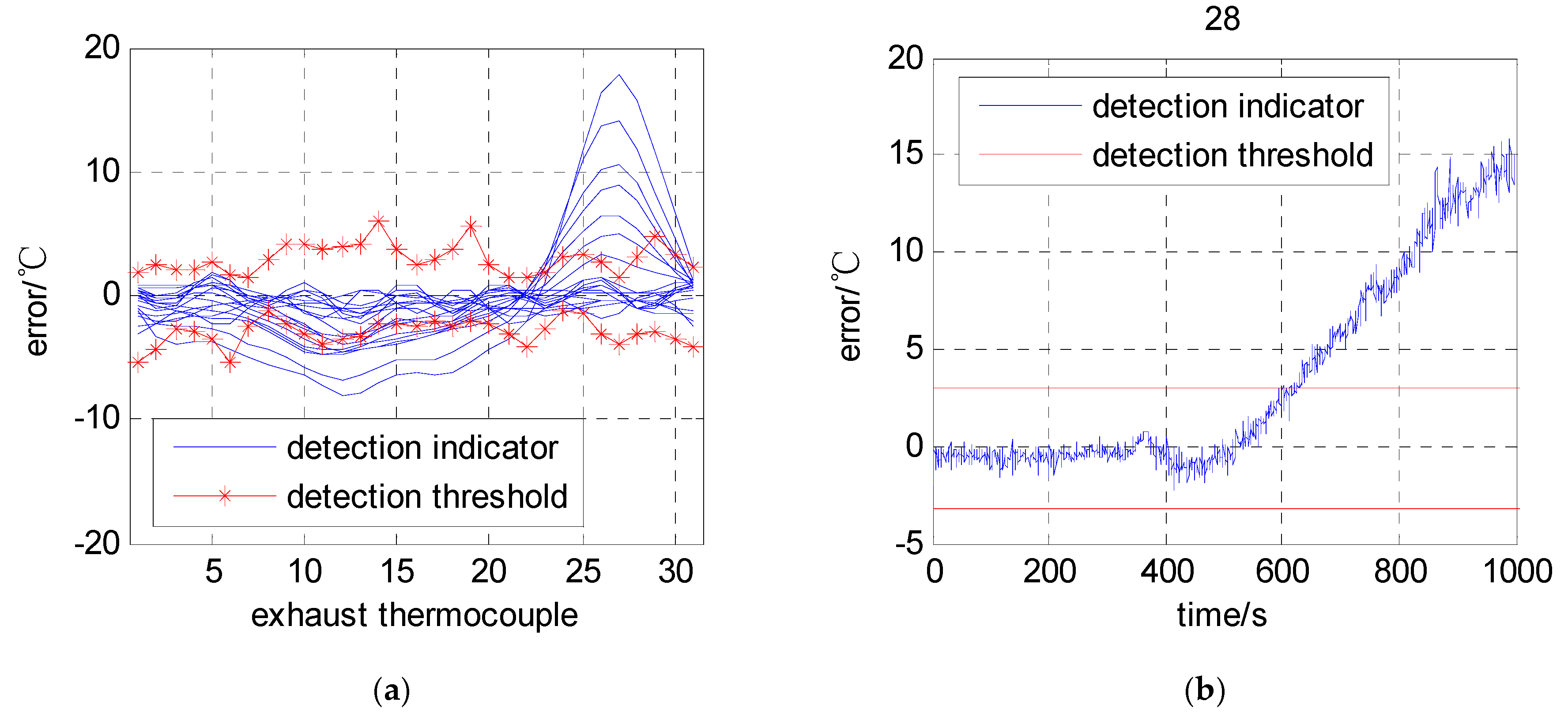
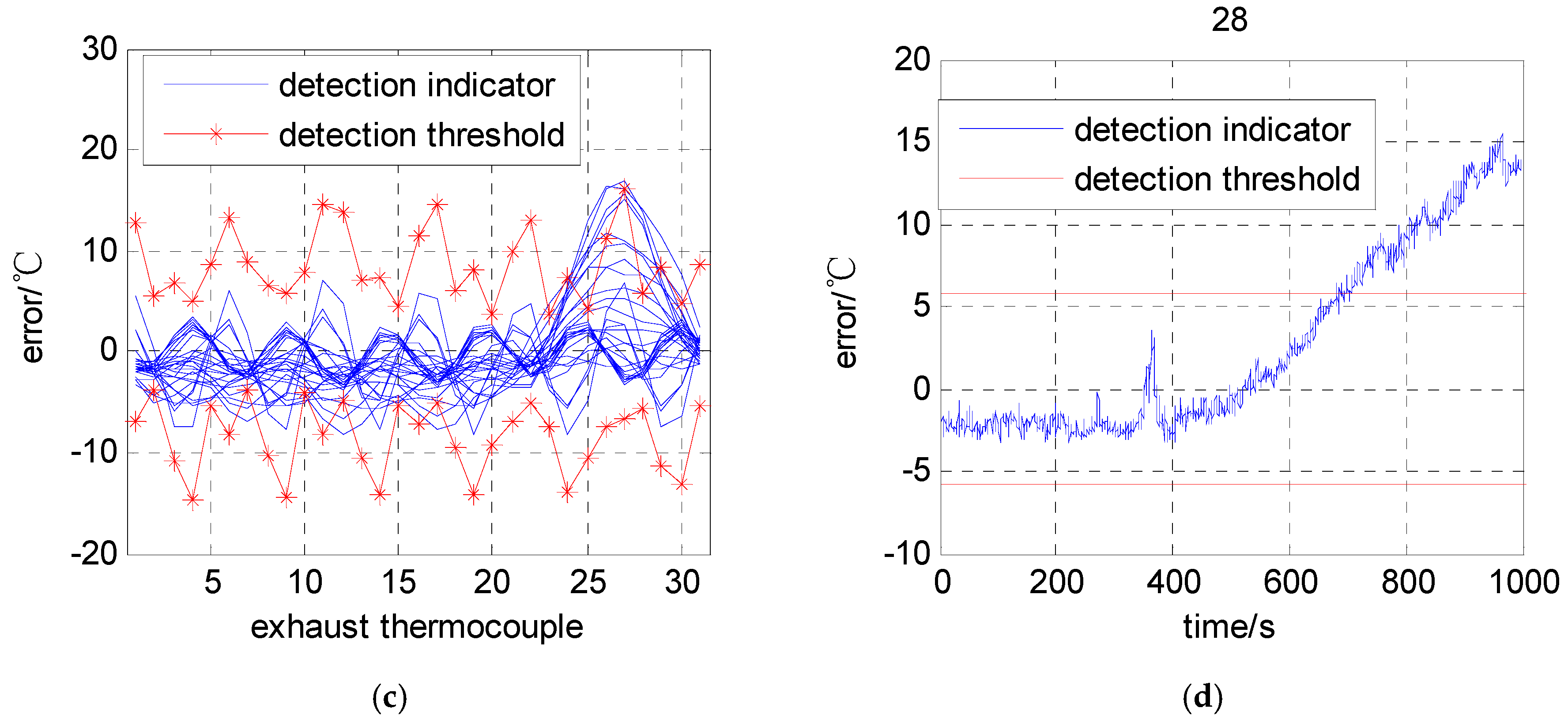
3.2. Fault Detection Result

In this section, the effectiveness of the proposed method, when used in hot component early fault detection, is stated. The methods with and without considering the swirl effect, as stated in Section 3.1, are compared by test dataset got from the simulation. EGT of the test dataset is shown in Figure 13, as the plant operates normally until 500 s, when the combustion efficiency of a combustor decreases slowly by 5%, as shown in Figure 14. The hot component early fault detection results by two models are shown in Figure 15. Since the error change near the 28th thermocouple in Figure 15a,c is the most severe, its error change is used for fault detection in Figure 15b,d. When the gas turbine is operating normally, the exhaust temperature error does not exceed the threshold. Both the models detect hot component early fault successfully, but the detection time of the model, which does not consider the swirl effect is longer because of a larger threshold value range. This means considering the swirl effect can improve hot component early fault detection sensitivity. Meanwhile, at about 380 s, when the gas swirl angle fluctuates to a relatively large value, the error of the model not considering the swirl effect also has a large fluctuation, but the other one remains stable error value. This further proved the fact that the method proposed in this paper can eliminate the influence of gas swirl on the exhaust temperature profile. It is also proved that the fault of one combustor has an influence on more than one exhaust temperature measuring result.

Because of the gas swirl effect, an exhaust temperature thermocouple measuring result reveals the performance of a different combustor. This is why the model based on multiple linear regression has larger error values when the swirl angle is relatively large. In contrast, the method proposed in this paper utilizes the internal relationship between the measuring points to establish the exhaust gas temperature distribution profile model. The variation of the operating and ambient conditions and especially the gas swirl effect is well-considered, and early fault detection sensitivity is improved effectively.

4. Conclusions

In this paper, a method used for early warning of gas turbine hot components is developed. The sensitivity of gas turbine hot components early fault detection is low because exhaust gas temperature is affected by not only faults but also the change of operating and ambient condition and gas swirl effect. When a fault is at an early stage, its influence on exhaust gas temperature is easy to be covered by other factors, which causes weak fault detection ability. From gas turbine basic principles, there is a relationship between exhaust gas temperature measuring points. In this paper, an exhaust gas temperature profile continuous distribution model is established. The model considers change of the operating and ambient conditions, and especially the swirl effect. The model is evaluated with the quantum particle swarm optimization (QPSO) method. The effectiveness of the method is tested by comparing it with another model based on multiple linear regression. As for the fault situation in this paper, the fault occurs at 500 s, the method, not considering swirl, exceeds the threshold at 680 s, while the method proposed in this paper exceeds the threshold at 600 s. Moreover, the accuracy rate of the method considering swirl reaches 90%, while that of the method not considering swirl is only 82%. The results show that the method proposed in this paper is more sensitive to hot components early fault when operating and ambient condition change or gas swirl effect happens. In other words, the method is not sensitive to the change of the operating and ambient conditions but still maintains sensitivity to the hot component faults.

References

1. General Electric Company. Heavy Duty Gas Turbine Monitoring & Protection; General Electric Company: Reno, NV, USA, 2015. [Google Scholar]
2. Yu, L.; Jin, J. Study on Deflection Laws of 9FA Gas-Turbine Exhaust Temperature Field. Electr. Power Constr. 2009, 3, 26. [Google Scholar] [CrossRef]
3. Gulen, S.C.; Griffin, P.R.; Paolucci, S. Real-time on-line Performance Diagnostics of Heavy-duty Industrial Gas Turbines. ASME J. Eng. Gas Turbines Power 2002, 124, 910–921. [Google Scholar] [CrossRef]
4. Liu, J. The Research for Exhaust Temperature Anomaly Detection in Gas Turbine. Master’s Thesis, Harbin Institute of Technology, Harbin, China, 2014. [Google Scholar]
5. Yılmaz, İ. Evaluation of the relationship between exhaust gas temperature and operational parameters in CFM56-7B engines. Proc. Inst. Mech. Eng. Part G J. Aerosp. Eng. 2009, 223, 433–440. [Google Scholar] [CrossRef]
6. Song, Y.X.; Zhang, K.X.; Shi, Y.S. Research on Aeroengine Performance Parameters Forecast Based on Multiple Linear Regression Forecasting Method. J. Aerosp. Power 2009, 24, 427–431. [Google Scholar]
7. Tarassenko, L.; Nairac, A.; Townsend, N.; Buxton, I.; Cowley, P. Novelty detection for the identification of abnormalities. Int. J. Syst. Sci. 2000, 31, 1427–1439. [Google Scholar] [CrossRef]
8. Yan, W. Detecting Gas Turbine Combustor Anomalies Using Semi-supervised Anomaly Detection with Deep Representation Learning. Cognit. Comput. 2020, 12, 398–411. [Google Scholar] [CrossRef]
9. Basseville, M.; Benveniste, A.; Mathis, G.; Zhang, Q. Monitoring the Combustion Set of a Gas Turbine. IFAC Proc. Vol. 1994, 27, 375–380. [Google Scholar] [CrossRef]
10. Zhang, Q.; Basseville, M.; Benveniste, A. Early warning of slight changes in systems. Automatica 1994, 30, 95–113. [Google Scholar] [CrossRef]
11. Medina, P.; Saez, D.; Roman, R. On Line Fault Detection and Isolation in Gas Turbine Combustors; ASME Paper No. GT2008-51316; ASME: New York, NY, USA, 2008. [Google Scholar]
12. Jinfu, L.; Jiao, L.; Jie, W.; Zhongqi, W.; Daren, Y. Early Fault Detection of Hot Components in Gas Turbines. ASME J. Eng. Gas Turbines Power 2017, 139, 021201. [Google Scholar] [CrossRef]
13. Talaat, M.; Gobran, M.H.; Wasfi, M. A hybrid model of an artificial neural network with thermodynamic model for system diagnosis of electrical power plant gas turbine. Eng. Appl. Artif. Intell. 2018, 68, 222–235. [Google Scholar] [CrossRef]
14. Chen, Q.; Li, H.; Li, M.; Xie, Z.; Xiu, J. Prediction of Aeroengine Exhaust Gas Temperature Based on RBF Neural Networks. J. Ordnance Equip. Eng. 2019, 6, 183. [Google Scholar]
15. Pi, J.; Huang, J.; Huang, L.; Gao, S.; Liu, G. Aeroengine Exhaust Gas Temperature Prediction Based on IQPSO-SVR. J. Vib. Meas. Diagn. 2019, 2, 18. [Google Scholar]
16. Zhang, Q. Contribution à la Surveillance de Procédés Industriels. Ph.D. Thesis, University of Rennes 1, Rennes, France, 1991. [Google Scholar]
17. Sun, J.; Feng, B.; Xu, W. Particle swarm optimization with particles having quantum behavior. In Proceedings of the 2004 Congress on Evolutionary Computation, Portland, OR, USA, 19–23 June 2004. [Google Scholar]
18. Camporeale, S.M.; Fortunato, B.; Mastrovito, M. A Modular Code for Real Time Dynamic Simulation of Gas Turbines in Simulink. J. Eng. Gas Turbines Power 2006, 128, 506–517. [Google Scholar] [CrossRef]
Figure 1. Combustors and thermocouples distribution.
Energies 13 05950 g001
Figure 2. Comparison between normal and abnormal operation.
Energies 13 05950 g002
Figure 3. Rotation of hot gas in a turbine.
Energies 13 05950 g003
Figure 4. Influence of exhaust gas temperature (EGT) profile swirl.
Energies 13 05950 g004
Figure 5. Swirl angle fitting result.
Energies 13 05950 g005
Figure 6. Residual of swirl angle.
Energies 13 05950 g006
Figure 7. Parameter process of quantum particle swarm optimization (QPSO) method evaluation model.
Energies 13 05950 g007
Figure 8. Parameter process of QPSO method evaluation model.
Energies 13 05950 g008
Figure 9. Exhaust temperature of train dataset (measuring points displayed in different colors).
Energies 13 05950 g009
Figure 10. Swirl angel of train dataset.
Energies 13 05950 g010
Figure 11. QPSO method optimal curve.
Energies 13 05950 g011
Figure 12. Comparison of error of fitting thermocouple exhaust temperature: (a) 4th thermocouple result; (b) 6th thermocouple result; (c) 25th thermocouple result; (d) 27th thermocouple result.
Energies 13 05950 g012aEnergies 13 05950 g012b
Figure 13. EGT of the test set (measuring points in different colors).
Energies 13 05950 g013
Figure 14. Fault combustion efficiency.
Energies 13 05950 g014
Figure 15. Detection results by two models: (a) Detection result considering swirl effect; (b) 28th thermocouple detection result considering swirl effect; (c) Detection result without considering swirl effect; (d) 28th thermocouple detection result without considering swirl effect.
Energies 13 05950 g015aEnergies 13 05950 g015b