Efficient Load Management for BEV Charging Infrastructure in Multi-Apartment Buildings

Abstract

Interest in and demand for battery electric vehicles (BEVs) is growing strongly due to the increasing awareness of climate change and specific decarbonization goals. One of the largest challenges remains the provision of large-scale, efficient charging infrastructure in multi-apartment buildings. Successful load management (LM) for BEV charging directly influences the technical requirements and the economic and environmental aspects of charging infrastructure and can prevent costly distribution grid expansion. The main objective of this paper is to evaluate potential LM approaches in multi-apartment buildings to avoid an increase in existing electricity demand peaks with BEV diffusion. Using our model parameters, off-peak charging achieved a 40% reduction in the building’s demand peak at 100% BEV diffusion compared to uncontrolled charging and reduced the correlation between BEV charging and the national share of thermal power generation. The most efficient charging capacity in the private network was achieved at 0.44 kW/BEV. A verification of the model results with the demonstration phase of the “Urcharge” project supports our overall findings. Our results outline the advantages of LM across a large-scale BEV charging network to control the impact on the electricity system along with the diffusion of e-mobility.

1. Introduction

Interest in and demand for battery electric vehicles (BEVs) is growing strongly. Reasons for this growth include increasing awareness of climate change, as well as the obligation of car manufacturers to reduce the CO2 emissions of their fleets substantially by 2030 [1]. One of the largest keys to success associated with this development is the provision of appropriate charging infrastructure (IS) [2]. Since BEV charging currently remains largely connected to single homes with private charging stations or charging at public stations, large-scale load management (LM) applications are still not commonly applicable. Major questions include not only where charging can take place (e.g., private and public charging, charging at work, etc.) and at which charging speed and capacity but also how the potential temporal distribution of this load behaves. The successful management of BEV charging demand is directly related to the economic aspects of charging IS installations and distribution grid performance and expansion requirements. This work is a result of the Austrian research project “Urcharge”, which aims at an extension of currently available LM functionalities for large-scale private charging IS at the technical, economic, and customer levels [3,4]. From a technical perspective, Urcharge aims at substantial enhancements of LM functionalities from a static management across a maximum of 15 sub-stations towards the dynamic management of more than 150 charging points, including improved data gathering and analysis, appropriate billing functionalities, and efficiency improvements. This is one of the few projects globally currently investigating private charging IS on such a large scale. Three projects in the US–in San Diego [5], Los Angeles [6] and Columbus–Ohio [7]–and one in Germany [8] aim at higher availability of BEV charging points in multi-unit dwellings.

For public fast charging, single-family buildings, and small company applications, many projects have already been conducted, with Hall et al. [9] providing a global best practice overview, IEA [10] describing the Nordic EV outlook, two projects for BEV charging IS in Denmark [11,12], and Project Better Energy in the UK [13], as well as one in Germany [14]. Nevertheless, our literature review reveals that research on large-scale charging IS with optimal load management (LM) in residential buildings remains scarce. Efficient LM is also referred to as smart charging in the literature, defined as an adaption of the BEV charging cycle to both the restrictions of the distribution grid and the needs of BEV users [15]. International Renewable Energy Agency (IRENA) [15] claims that smart BEV charging enables peak shaving, network congestion management, and reduced grid capacity investments. Various studies cover research on the electricity demand profiles of BEVs and potential peak increases. Van Vliet et al. [16] discovered the negative effects of uncontrolled BEV charging on the distribution grid and found that with a BEV diffusion of 30%, the Dutch peak electricity demand would grow by 7%, and the household (HH) or overall building peak demand would grow by 54%. Several studies observed the benefit of off-peak charging, in which the base load is increased while the national peak load remains untouched. While van Vliet et al. [16] highlighted the benefit of off-peak charging for the energy use cost and CO₂ emissions of BEVs, Bitar and Xu [17] suggested a price that decreases with the deadline that is granted by the user for the completion of the charging process. Limmer and Rodemann [18] highlighted the cost aspects of peak charging at public stations. They argued that although the majority of public charging stations for BEVs are presently uncontrolled, controlled charging should offer a price that decreases with the latest deadline the user allows for charging to increase the availability of the BEV at the station. From our perspective, however, this pricing-scheme requires an appropriate interface for the user and would lead to parking lots being blocked for a considerable amount of time. This scheme, therefore, is designated for applications with an assigned parking lot.

Several studies on LM for BEV charging widely address pricing mechanisms to limit negative effects on the distribution grid. Some suggest a time-of-use (ToU) pricing mechanism that incentivizes off-peak charging with a lower charging price [19,20]. New peaks, however, may still arise if too much charging power is pushed into off-peak times. Therefore, so-called dynamic load-based pricing is a potential solution in which charging power decreases with the amount of BEVs charged at a time [17,19]. Dynamic pricing while the BEV is already plugged in, however, represents high price uncertainty and would need to be based on a forecast of charging demand. It has to be kept in mind that such an LM or restrictions on charging power can also be implemented top-down from the control station across the charging points to guarantee distribution grid performance. On the other hand, Yan et al. [21] found that traffic jam and weather forecasting can enhance the operation of LM. Temperatures have an impact on battery performance and heating and cooling demands, while the traffic conditions influence the electricity consumption of driving.

Recently, an increasing number of studies has been published concerning the impact of e-mobility on the distribution grid, power quality, and power generation capacities. Crozier et al. [22] observed that controlled charging has a significant benefit for Great Britain’s electricity network. It can reduce expansion requirements for electricity generation capacities, as well as investment into the distribution network. Das et al. [23] focused on the grid integration of BEV charging IS, whereas Khalid et al. [24] emphasized the power quality aspects in the utility grid and Brinkel et al. [25] analyzed the need for grid reinforcement because of growing e-mobility. The benefits of controlled charging have also been discussed within the context of smart grids and smart cities, in which an optimal charging scheduling is carried out to improve grid system operation, voltage, and efficiency [26,27]. Another paper developed an optimized charging framework using knowledge of the upcoming trip schedule of the BEVs [28]. However, such detailed information is difficult to obtain.

Using the battery of the BEV to switch flexibly between charging and providing energy to the power grid has been analyzed from various perspectives throughout the last decade. Some focus on the potential of vehicle-to-grid (V2G) for BEV integration into smart grids [29,30] and its impact on the grid in general [31]. From a user perspective, V2G sometimes is regarded as the potential missing link for the acceptance of BEVs as a cost-effective support policy. Chen et al. [32], for example, found that in Nordic countries, V2G capability—apart from charging time—is a technical aspect that improves BEV adoption. Sortomme and El-Sharkawi [33] studied optimal charging strategies for V2G application. Various studies, however, analyze the techno-economic feasibility of V2G [34,35,36] and find that, economically, this strategy may only be feasible in specific scenarios which highly depend on the battery degradation costs related to V2G cycling. Noel et al. [37] and Parsons et al. [38] investigated the willingness to pay for V2G applications and concluded that V2G is only relevant in countries with higher overall education or knowledge of the technology. Furthermore, the concept needs to provide a financial incentive for the user to be successful. While Habib et al. [39] studied the impact of V2G technology and charging strategies on the distribution network, the parker project represented a field test of V2G infrastructure and found that V2G can be commercialized by providing frequency containment reserves [40]. Rezania [41] even concluded in a study on Austria that, from an electricity system point of view, the participation of BEVs can hardly be competitive in the frequency reserve market. The competition from other providers with technological and cost advantages, such as heat pumps and pumped hydro, is too strong and the battery degradation cost limits the potential economic benefit.

Some recent studies also investigate in the ability of LM to reduce greenhouse gas (GHG) emissions and promote the integration of variable renewable energy (VRE). Apart from the cost and emission optimization of BEV charging by Brinkel et al. [25], Tu et al. [42] optimized BEV charging to minimize the emissions from electricity consumption. Additionally, Dixon et al. [43] modelled a BEV charging schedule that minimizes carbon intensity and seeks to absorb otherwise curtailed renewable electricity. Their method achieved an average 25% reduction of the CO₂/km compared to uncontrolled charging from Great Britain’s grid.

Nevertheless, despite this technique’s great potential, limited work is available that focuses specifically on private BEV charging IS and the potential of large-scale LM in multi-apartment buildings. Lopez-Behar et al. [44] claim that in many cities, most of the residents live in multi-apartment buildings not yet equipped with proper BEV charging IS. Simulation results based on real-world driving data by Wang et al. [45] show that home charging is able to meet the energy demands of the majority of BEVs under average conditions. Kim et al. [46] analyzed residential BEV charging behavior. Additionally, Yi et al. 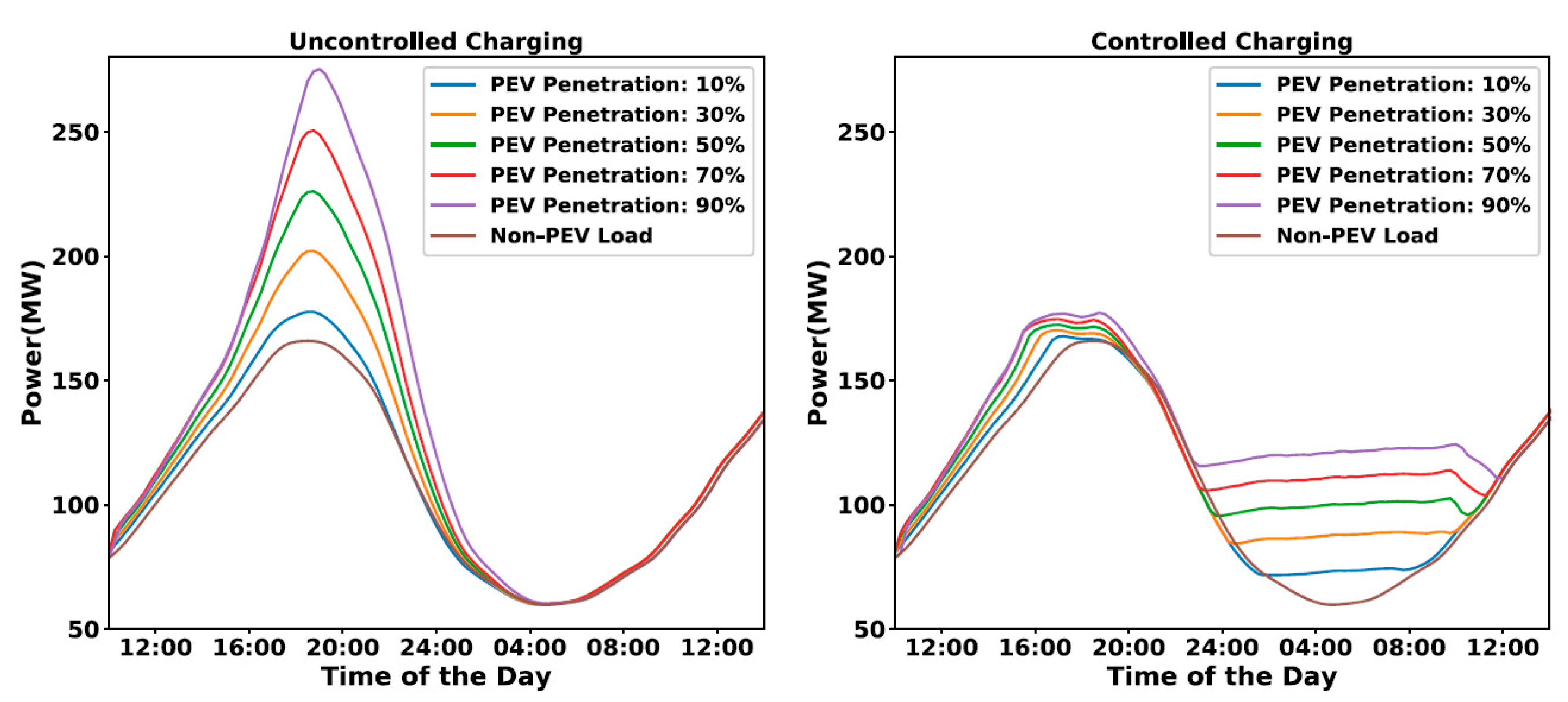[20] optimized the charging of BEVs via charging behavior models based on a real-world data set of a Nissan Leaf during weekdays, measured from thousands of charging points over several years. The authors found that BEV charging tends to occur together with distribution grid peak loads. Five different scenarios with varying BEV penetrations were simulated to show the difference between uncontrolled and controlled charging (Figure 1). Each scenario includes 100,000 HHs and considers BEV penetrations between 10% and 90%. Jang et al. [47] eventually optimized residential BEV charging to avoid peak loads and minimize charging cost for the user and Khalkhali et al. [48] investigated a residential smart parking lot to control grid performance.

The main objective of this paper is to evaluate the potential LM approaches for BEV diffusion to avoid an increase in existing HH electricity demand peaks in multi-apartment buildings and thus substantial long-term, system-wide capacity investments and operational costs. While the 6-month demonstration phase within Urcharge tested LM for 51 BEVs representing 50% E-mobility in this area, our model provides a framework to analyze the impact on electricity demand profiles up to 100% E-Mobility. We compare the situation of uncontrolled charging to the results with LM approaches and address the environmental effects of a substitution of conventional cars with BEVs and their electricity consumption. Another important goal within this analysis is to define the minimum charging capacity required for each BEV (kW/BEV) as an indicator for cost-efficient sizing. Once the power connection assigned to the area is exceeded by the HH plus BEV electricity demand, substantial costs occur to reinforce the power cables or even buy additional power capacity from the grid operator. Our contribution mainly benefits from being embedded in a holistic research project for Austria, and our model results are verified by experience from the project’s demonstration phase in Section 4.2.

This paper begins with a description of our methodology, model parameters, and assumptions and the considered charging strategies. In Section 3, we present the results of this research. We also describe the existing HH electricity demand, and the impact of E-mobility with uncontrolled BEV charging, compared with the changes through LM and the minimum required charging capacity for each BEV. Finally, in Section 4, we carry out a detailed discussion of our modelling results with a verification using the monitoring data from the project demonstration phase in Section 4.2. The environmental impact of E-mobility is evaluated in Section 4.3, and Section 5 provides the comprehensive conclusions of our work.

2. Materials and Methods

To analyze the impact of different LM approaches on the building’s electricity demand, we first define a yearly HH load profile for a residential area with 106 households. The BEV charging demands and availability times at home or public charging points, depending on the trip’s start time and length, are taken from a modeling paper by Hiesl et al. [49] based on an Austrian traffic survey. The approach is briefly outlined in Section 2.2. Our model coordinates individual passenger BEV charging in the home network according to the constraints for each charging scenario (Section 2.3.1). The results allow assessing the impact of LM on large-scale BEV charging on electricity demand peaks and valleys. The model parameters largely reflect the common technical standards on battery capacity, charging speed, and efficiency for private stations.

On the one hand, our model analysis is subject to simplifications from more detailed, real-world technical functionalities to enable more generally applicable conclusions. On the other hand, it helps us to carry out additional analyses that were not tested throughout the Urcharge demonstration phase and draw conclusions on the impact of E-mobility toward 100% BEV diffusion. Simplifications to the model include the operation of the LM optimization model under full information of BEV electricity consumption and the trip start times across one year, as well as the assumption of one uniform battery size and uniform technical characteristics for all BEVs. Furthermore, our model operates under knowledge of the battery’s state of charge, which is currently not the case in a real setting. A detailed description of the differences between the modeled and real environment in the project, as well as a verification of the model results, are provided in Section 4.2. The model does not cover any load flows of the distribution grid or V2G approaches but instead focuses on an analysis of potential LM approaches to reduce the impact of e-mobility on the overall building load.

2.1. Household Electricity Demand

For our analysis, the electricity demand profile throughout the day is of greatest importance. Of course, demand may vary with parameters such as the HH size and the habitants’ ages and types of profession. Furthermore, the HH electricity demand profile is subject to changes due to increasing electrification. However, we only considered the relative impact of e-mobility on existing building electricity demand and did not model any future scenarios.

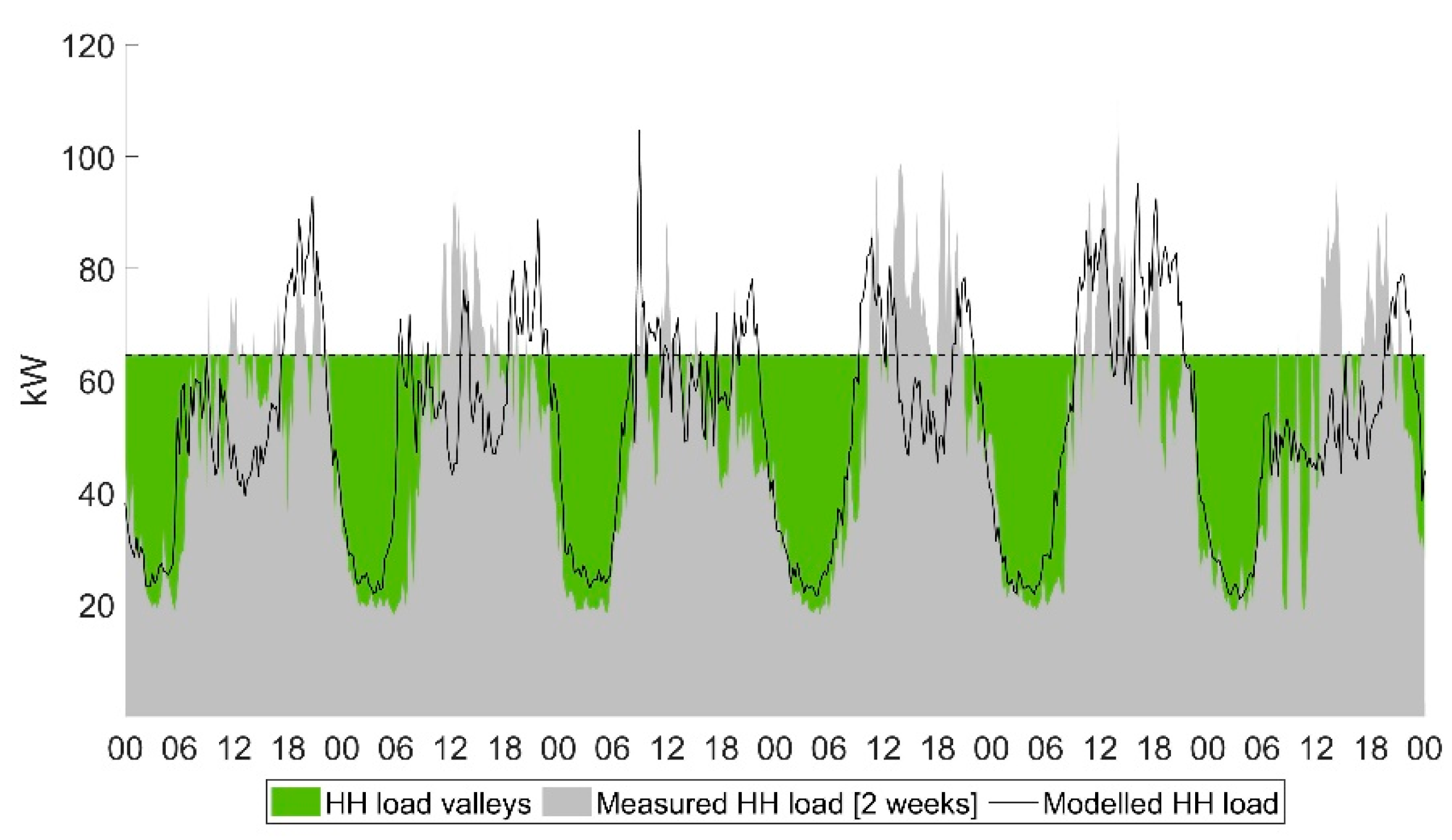
To determine the aggregate HH electricity demand that largely resembles the demonstration site’s 106 HHs, two weeks of data were measured on-site at the respective building’s power connection. To achieve a realistic yearly profile for our model, an alternative yearly dataset from a similar project was used. We extrapolated this alternative yearly dataset to the demand level during the measured two weeks at the Urcharge demo site such that the average electricity demand during the same two-week time periods matched. Eventually, the patterns were similar, and the adapted yearly data were considered feasible for our study. The two weeks of measured Urcharge HH electricity demands and the aligned yearly data are shown in Figure 2.

For our further analysis, a threshold to differentiate the HH load valleys and peaks using the 70th percentile (P70) was defined, which is also described in Figure 2. This parameter represents the threshold that 70% of all HH load values lie below, which is 64.5 kW. Then, the LM approaches mostly aim at minimizing the impact on the peaks or shifting BEV charging demands in the HH load valleys. The detailed approaches for LM are described in Section 2.3.1.

The impact of e-mobility on the existing building electricity demand and the effectiveness of LM approaches was evaluated according to the specific indicators determined to be appropriate, as described in

Table 1. Important result parameters (see Figure 2).

Parameter	Description
Maximum demand (kW)	Maximum electricity demand discovered in the year
Minimum demand (kW)	Minimum electricity demand discovered in the year
Peak demand volume (MWh)	Electricity demand volume exceeding the P70 threshold
Base demand volume (MWh)	Electricity demand volume within the HH load valleys beneath P70

.

2.2. BEV Driving Profiles

To determine common BEV charging demands, the driving profiles according to Hiesl et al. [49] are applied, which were derived from an Austrian traffic survey [50], as a static input for our optimization model. Eight typical driving purposes with the relevant distribution of common distances, related electricity consumption, and potential start times for urban Austrian car users were applied to determine when and after which level of energy consumption each BEV is parked and ready to charge within the private IS [50]. The modeled energy consumption aims at meeting the traffic survey results for Austrian cities (excluding Vienna) with an average yearly distance traveled by each driver of 12.237 km/a.

BEV consumption is modeled as an interpolation between 15 kWh/100 km in summer and 17 kWh/100 km in winter due to the additional power consumption for heating and the temperature sensitivity of the batteries [51]. Due to computing performance, the model calculates the distribution of BEV charging availability for 10 different BEV profiles. Assuming one parking lot for each HH, we extrapolated these charging profiles to the number of BEVs for specific percentages of BEV diffusion according to

Table 2. Number of BEVs in the modeled multi-apartment building for BEV diffusion.

No. of BEVs	BEV Diffusion
11	10%
32	30%
53	50%
80	75%
106	100%

.

2.3. Optimization Model

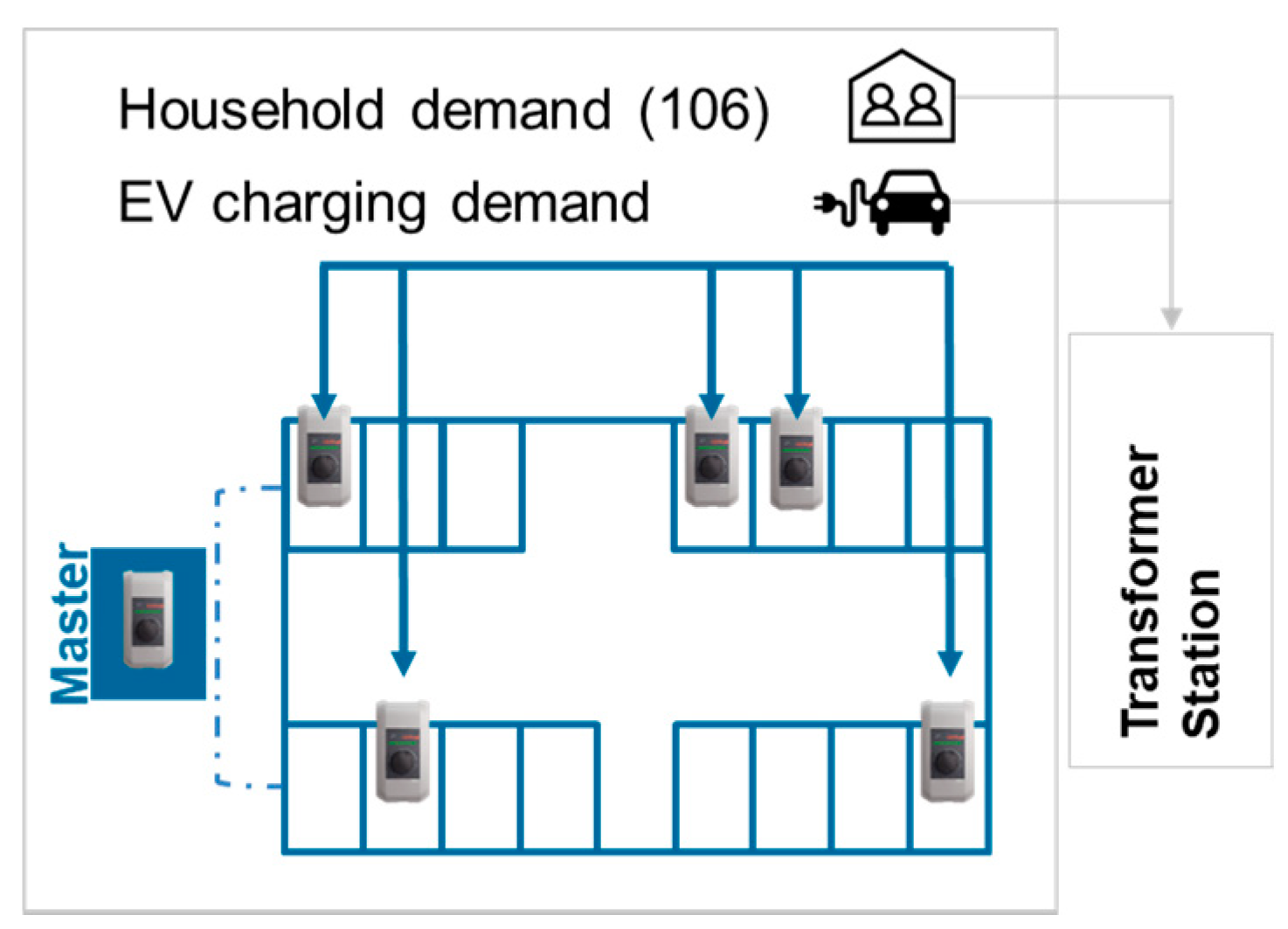
The BEV charging demand is controlled within a charging network including one central control or master station, thereby coordinating charging for each private sub-station in the area (Figure 3).

The maximum charging power of private stations is defined as 3.7 kW, whereas public charging stations operate at 22 kW. 3-phase charging is not examined, with which a vehicle can charge at a speed of 11 kW (3 × 3.7) at home, but only 1-phase charging. The battery capacity of the individual passenger BEVs is set to 40 kWh. We do not aim at modeling a specific vehicle model. The current battery state of charge is determined by the state at the end of the former time step and the energy consumed and charged in the current time step.

Our model optimizes private charging in 15 min time-steps based on the full information of the yearly BEV power consumption, potential charging times, and HH load and is established as a linear optimization model. The objective function aims at minimizing the costs of BEV charging $({\mathrm{c}}^{\mathrm{ch}}$) depending on the cost (c) and consumed charging power (p) at the home (h) and public (p) charging point in each time step t (see Equation (1)). The BEV demand is a static input to this LM model from Hiesl et al. [49] and depends on the distance traveled for each driving purpose and the respective electricity consumption (see Section 2.2). Overall, charging should primarily be carried out within the private, controlled network, while public charging should only take place at times of urgent need.

$$\underset{\begin{array}{c}\left\{p_t^p{, p}_t^h\right\}\\ {\{c}_t^p{,c}_t^h\}\end{array}}{\mathit{min}}{\mathrm{c}}^{\mathrm{ch}}\left(p, c\right)$$

(1)

This objective function derives the optimal allocation of charging power across all time steps to fulfill the BEVs demands within the constraints for each BEV charging scenario described in Section 2.3.1. This function aims at recharging the BEV before the next journey starts. Obviously, reality this far does not provide any information on the upcoming consumption of the BEV. Nevertheless, modeling with full yearly information offers valuable insights into the benefits of exact customer information.

2.3.1. Charging Strategies

The BEV charging strategies represent different approaches for the control of charging power by the master station top–down across all charging points (Figure 3). We use an uncontrolled charging scenario, without any control measure, as a reference. This represents the start of charging once the BEV is plugged in at the home station. Then, these results are compared to the expected improvements with two LM approaches aimed at a specific distribution of BEV electricity demand. For all charging approaches, it is assumed that the BEVs are plugged in and available for charging while parked at home.

The following BEV charging approaches are being analyzed:

• Uncontrolled charging (UC)
  As a reference scenario, there are no LM measures applied.
• Low charging capacity (LCC) LM approach
  The LCC approach refers to slow charging at very low charging power for each BEV to avoid excessive peaks in charging demand. Charging is operated a high simultaneity rate.
• Time-of-use (ToU) LM approach
  With the ToU approach, the master station shifts BEV charging power from the HH load peaks into the valleys, as described in Figure 2. The HH load peaks are defined as any value exceeding the threshold P70 (see Section 2.1).

As important indicators of the impact of different charging strategies on the distribution of charging power and the length of charging processes, we analyze the simultaneity factor, the average charging power applied, and the charging time ratio. These factors are also compared to the results of the project demonstration phase in Section 4.2.

• Simultaneity factor
  The simultaneity factor describes the average amount of vehicles charging at the same time across the whole year. Therefore, LM approaches that promote longer charging time periods result in a higher factor of simultaneously charging BEVs.
• Charging time ratio
  This indicator relates the time a vehicle is charged to the time it is parked. This factor is expected to be much higher for the LM scenarios ToU and LCC than for the uncontrolled approach, which leads to shorter charging time periods at higher charging power.
• Average and maximum charging power
  The average charging power refers to the average power the BEV is charged at during active charging. We also analyze the maximum charging power to reveal the charging load peak, which is an indicator for the speed at which charging is processed. It is assumed that uncontrolled charging, that does not promote the management of charging power, will lead to a higher average charging power than the ToU or LCC approach.

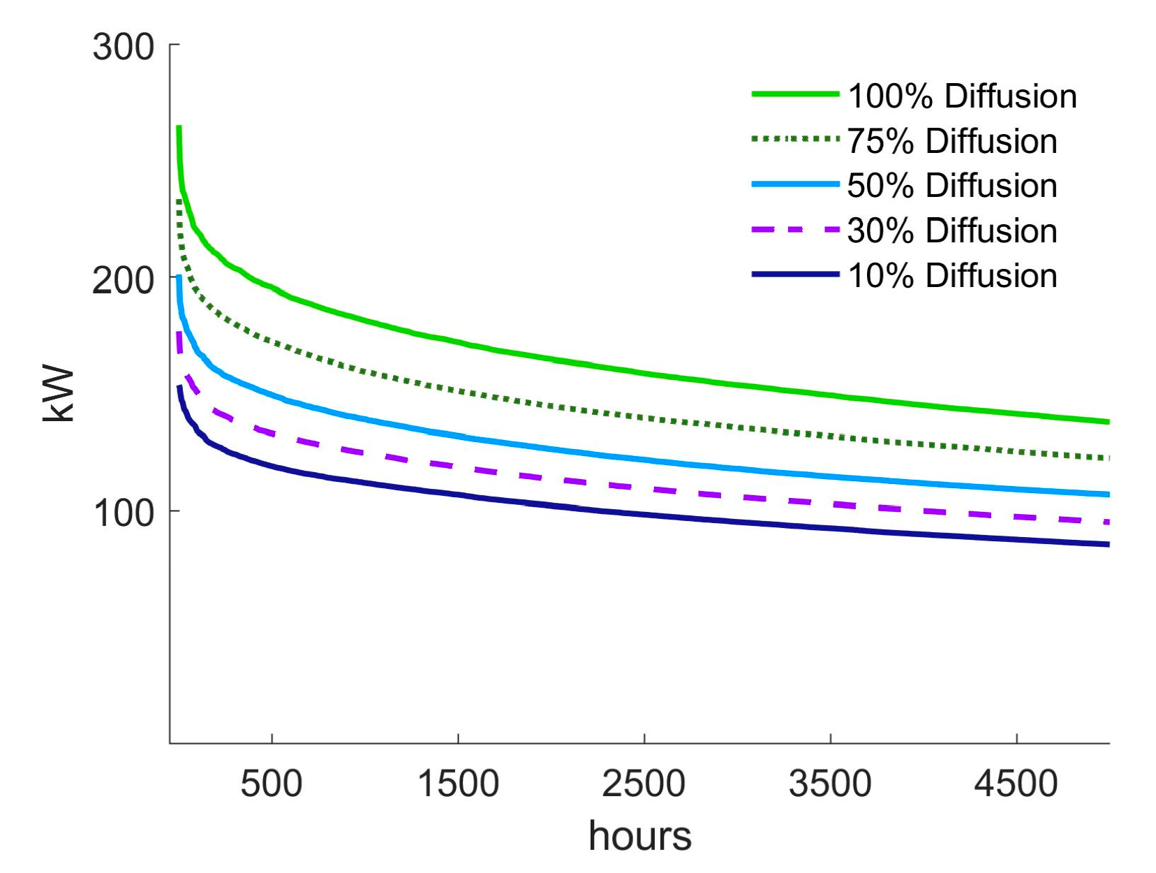
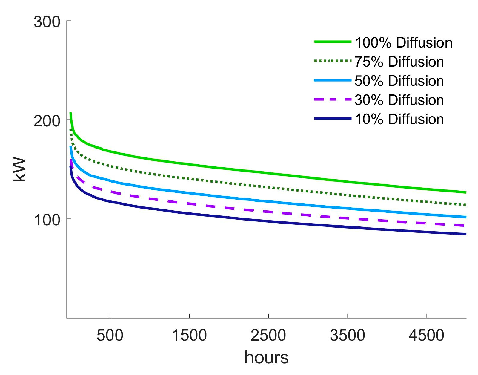
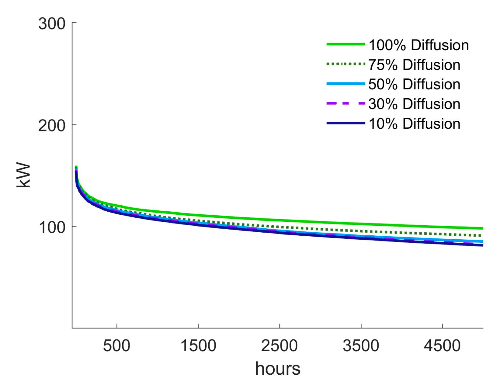
2.4. Minimum Charging Capacity

Determining the charging capacity required for each BEV involves an investigation independent of the optimization described in Section 2.3. This analysis can reveal the most efficient sizing for charging capacity down to a level at which there is no flexibility left for load shifting. This means an operation at the highest simultaneity of charging processes at the slowest possible speed resulting in the highest distribution of charging power across time.

The cost for charging capacity for the whole area is subject to step fixed costs, which increase substantially once the regional power connection capacity needs to be expanded. This analysis uses the objective function described in Equation (2) to minimize the average charging power ($p_{}^h)$ consumed across the number of all charging points (n) in each time step (t). The minimum charging capacity that needs to be installed for the charging network is derived from the highest charging power consumed by the sum of all home charging points across a year (see Equation (3)). To eliminate outliers in the BEV electricity demand from rare very high BEV electricity consumption due to few long-distance trips, the highest 5% of charging power consumed are removed. Then, this aggregated capacity is divided by the amount of charging points to arrive at the desired indicator kW/BEV. This indicator represents the minimum charging power for each BEV required to fulfill the demand throughout the year.

Two modeling approaches representing different levels of information are applied: yearly optimization with full information and daily rolling optimization. For the daily approach, a higher required minimum capacity is expected due to the inability to balance charging over more than one day.

$$\underset{\left\{p_{n, t}^h\right\}}{min}{\displaystyle \sum }_n{p}_t^h$$

(2)

$${cap}^{h }= max ({\displaystyle \sum }_n{p}_t^h)$$

(3)

2.5. Environmental Impact of e-Mobility

Considering the results of the former analyses, the environmental impact of e-mobility in the considered residential area are evaluated based on the following aspects:

• Savings in GHG emissions from the substitution of fossil-fuel-powered vehicles with BEVs

The savings in CO₂-eq, particulate matter (PM), and nitrogen oxide (NOx) are analyzed through the continuous substitution of conventional vehicles using diesel- or petrol-powered internal combustion engines with BEVs across the whole life cycle from vehicle and battery construction to energy provision and driving. This is based on the average yearly km traveled by each car from our model results and the Austrian data on specific emissions for each type of fuel [52]. Scenarios on the future development of individual transport, such as a shift to public transport or bicycles along with the energy transition or an increase in BEV use resulting from a rebound effect due to driving without regret of air pollution are not included. The emissions are based on current measures and will likely decrease further in the future for conventional and battery-powered vehicles. The CO₂-eq emissions are 178 g/km for diesel and 225 g/km for petrol-powered vehicles. However, diesel includes much higher amounts of NOx, with 0.385 g/km compared to petrol with 0.162 g/km. PM emissions amount to 0.021 g/km and 0.024 g/km for diesel and petrol, respectively. The Austrian shares of diesel and petrol vehicles from the stock of 2019 are applied, whose diesel share of 56% is much higher than the European average [53].

According to the Austrian climate goals, by 2030, national electricity generation must be 100% renewable ([54,55]). For our scenario of 10% BEV diffusion, which represents the status in 2020, we, therefore, use the specific emissions of the current Austrian electricity mix represented in the UBA scenario “BEV(Aut-Mix)” [52]. Between 30% and 100% BEV diffusion, representing the situation from 2030 onwards, the electricity consumed is assumed to be almost fully renewable with specific emissions, as in the UBA “BEV(UZ-46-Mix)” [52] scenario.

2.

Impact of LM on the environmental aspect of the electricity mix consumed for charging

Based on the correlation between the Austrian fossil electricity generation ($p_{\mathit{foss}}$) from coal and gas [56] and the BEV charging power consumption ($p_{\mathit{ch}}$) from the model, we evaluate the potential effect on the environmental aspect of electricity consumption:

$${\mathrm{r}}_{\mathrm{foss}}= \frac{{\mathrm{Cov}}_{p_{\mathit{ch}}, p_{\mathit{foss}}}}{{\mathsf{\sigma }}_{p_{\mathit{ch}}}{,\mathsf{\sigma }}_{p_{\mathit{foss}}}}.$$

(4)

3.

Environmental impact of E-mobility and LM on potential grid expansion

From the resulting impact of uncontrolled and controlled charging on the maximum and peak demand, as well as the importance of the minimum charging capacity, conclusions on the consequences for grid expansion and its environmental effects are derived.

3. Results

The modeling results in this section are structured as follows.

Section 3.1 describes the existing HH electricity demand as a basis to evaluate the impact of e-mobility on the building load. Section 3.2 and Section 3.3 show the effects of BEV charging with uncontrolled charging and by applying the LM approaches (LCC and ToU). Section 3.4 addresses the minimum charging capacity that must be available for each BEV. In general, we observe that throughout the diffusion of e-mobility up to 100%, the model mainly uses the private charging network, while public charging only fulfills up to 3% of the yearly demand. Therefore, we conclude that the sufficient availability of efficient private charging IS reduces the need for fast charging options, at least for common daily business.

3.1. Household Electricity Demand Characteristics

The HH electricity demand is the basis for our analysis of the impact of increasing BEV diffusion and has a duration curve, as shown in Figure 4. The yearly total demand accounts for 487 MWh, and the profile shows the characteristics outlined in

Table 3. Household load characteristics.

Parameter
Maximum demand (kW)	153.8
Minimum demand (kW)	19.2
Peak demand volume (MWh)	49.2
Base demand volume (MWh)	437.6

.

While the LM approaches aim at minimizing an increase in the building’s maximum and peak volume demand through e-mobility, a successful shift into the HH load valley will result in an increase of the minimum and base volume demand (see Figure 2). This will result in a more balanced daily building demand profile with less variability. On the one hand, this can mean greater predictability and stability in the building load profile for the distribution grid. On the other hand, the increasing electrification of a growing number of applications could result in additional or new peaks in the future. However, the HH load valleys largely coincide with the overall national electricity demand valleys. Therefore, a BEV load shift into these times may avoid the expansion requirements for the distribution grid and electricity generation capacities for a reasonable amount of time. The material production, infrastructure implementation, land-use associated with the installation of power plants and cables, and disposal obviously entail substantial environmental and economic impacts.

3.2. Uncontrolled Charging

As explained in the introduction, charging without any load control mechanism increases electricity demand peaks, showing a strong correlation between the electricity demand for BEV charging and that for the HHs. Without any LM approach, most BEV users return home during the evenings and immediately plug in their vehicle for charging. Figure 5 shows the impact of BEV charging on electricity demands without control for an exemplary day along with the diffusion of e-mobility. In this uncontrolled scenario, only 50% of all vehicles charge at the same time (simultaneity factor) and on average, the vehicles only charge 9% of the time they are parked (charging time ratio). The latter proves the short time period during which charging is completed, which implies high charging power in the uncontrolled scenario. The average charging power consumed per BEV is 0.40 kW, and the maximum charging power consumed accounts for 1.80 kW.

The impact of uncontrolled BEV charging on the electricity demand peaks becomes even more visible in the duration curve shown in Figure 6, where the total building electricity demand (BEV charging plus HHs) is ranked from the highest to the lowest for the highest 4500 h in a year. This curve reveals a remarkable increase in the building’s maximum and peak volume demand along with growing e-mobility. Toward 100% BEV diffusion, the maximum electricity demand increases by 72% from 153.8 kW without e-mobility to 265.2 kW, and the peak volume demand grows almost four-fold. This increase in peak electricity demand may have severe consequences for the distribution grid and capacity investment in the area. The minimum electricity demand remains untouched, since charging usually coincides with higher HH electricity demand. The base volume demand also only increases by 20% up to 100% BEV diffusion. Therefore, the next section outlines the advantages of the defined LM approaches.

3.3. Load Management Scenarios

LM can have a significant impact on the characteristics and distribution of the BEV electricity demand profile. If the BEVs are available for charging for a sufficient amount of time, the charging demand can successfully be shifted away from the HH load peaks into the valleys, as indicated in Figure 2. The results of the two LM approaches are also compared to uncontrolled charging. A more detailed quantitative discussion of all charging strategies is provided in Section 4.1.

Figure 7 shows the results for the LCC approach whose slow charging speed leads to a greater BEV load distribution over time compared to uncontrolled charging. In this scenario, on average, 86% of all vehicles charge at the same time, and the vehicles charge 16% of the time they are parked. This represents very long charging times and great simultaneity, though at substantially reduced charging power. The charging times still correlate with the evening HH load peaks. Nevertheless, the extreme peaks in the evening times experienced with uncontrolled charging are reduced substantially with the limitations on overall charging capacity. The duration curve of the building electricity demand in Figure 8 reveals a much smaller peak increase throughout BEV diffusion with a steadier distribution of BEV charging power compared to uncontrolled charging.

The ToU approach achieves the best results in shifting the charging demand away from the HH load peaks (see Figure 9). On average, 81% of all vehicles charge at the same time, which is a bit less than with the LCC approach, and again the vehicles charge 15% of the time they are parked. For both LM approaches, the average charging power consumed per BEV is cut down to 0.24 kW; this is only half of that with uncontrolled charging, and the maximum charging power consumed only accounts for 0.67 kW. This clearly proves the greater distribution of BEV charging power with the LM approaches. The duration curve in Figure 10 proves the capability of this approach to minimize the impact of e-mobility on electricity demand peaks in the building. Here, we observe an increase of only 4% in the yearly maximum demand under the full diffusion of BEVs.

3.4. Minimum Charging Capacity

Using our approach described in Section 2.4, first the minimum charging capacity for each BEV is calculated applying yearly optimization with full information. The yearly information of charging demand allows for a very efficient dimensioning of charging capacity. The minimum charging capacity that needs to be available accounts for 0.44 kW/BEV. However, charging mostly takes place at home, and only 4% of the BEV power demand is covered by public stations. Figure 11 depicts the resulting distribution of BEV charging demand, which largely relies on the availability of BEVs over time.

If now daily rolling optimization is applied, charging can only be carried out based on the information available for one day, without any knowledge of later demand. In our model, less information leads to a substantially higher minimum charging capacity of 1.3 kW/BEV. This capacity can result in higher costs for IS implementation. Hence, even foresight into the next day could help provide more flexible charging and integrate important aspects into the LM process, such as a positive weather forecast leading to longer weekend trips or an alignment of charging with renewable power availability. The efficient sizing of charging capacity reduces the risks and costs associated with exceeding the available regional power connection and thus guarantees a fair price to the final user for private charging.

4. Discussion

In this section, the modeling results are discussed in detail and the environmental implications of e-mobility and the advantages of LM are evaluated in this context.

4.1. Impact of LM on BEV Charging Profiles

Here, the development of each parameter defined in Table 1 for BEV diffusion under the different charging strategies (UC, LCC, and ToU) is discussed and the results are compard to the situation without any e-mobility (see the HH load characteristics in Section 3.1). In general, we find that the simultaneity of charging, which indicates how many BEVs charge at the same time, increases from 9% under uncontrolled charging to 16% under both LM approaches. The charging time ratio increases from 50% to 86% between uncontrolled charging and the LCC approach. Both factors indicate the ability of LM to achieve longer charging periods at lower charging power.

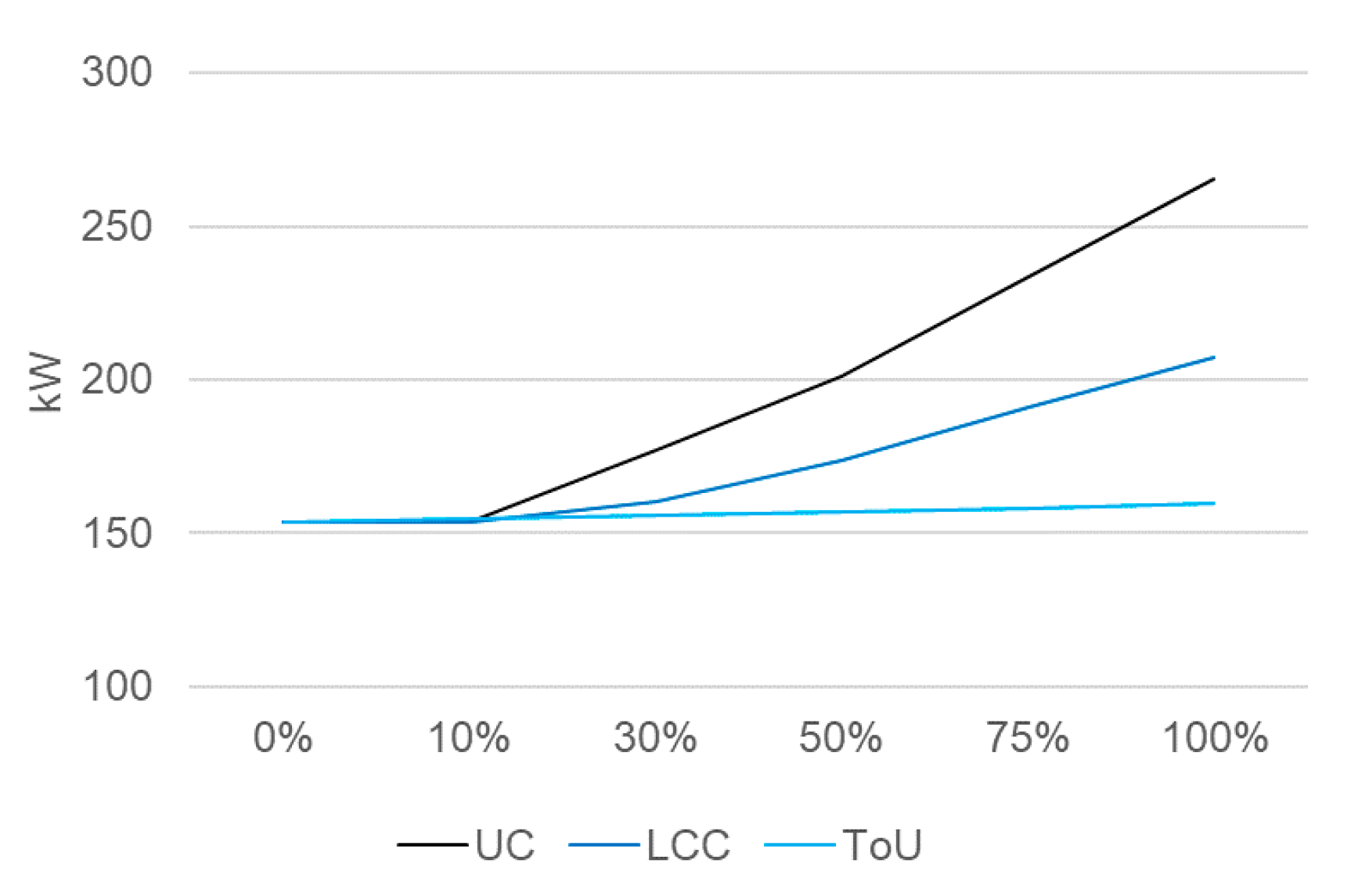
Figure 12 shows that while uncontrolled charging (UC) leads to a rise in the detected yearly maximum electricity demand up to 100% BEV diffusion of 72%, reaching 265 kW, a restriction in the charging capacity with the LCC approach already achieves some reductions. With the LCC approach, the maximum demand reaches 207 kW with the full diffusion of BEVs—which is an increase of 35%—but it hardly increases at all until 50% BEV diffusion. The ToU approach almost manages to keep the electricity demand below the existing HH maximum demand, which only increases by 4% with full BEV diffusion. This way, e-mobility has hardly any impact on the yearly maximum demand.

The peak volume demand, which represents the sum of the demand above the P70 threshold, rises exponentially for all charging strategies between 50% and 100% BEV diffusion (see Figure 13). The uncontrolled scenario leads to a yearly peak volume of 236 MWh up to full BEV diffusion—a fourfold rise compared to no e-mobility. While the LCC still results in a threefold increase up to 193 kWh, the ToU approach achieves a successful shift in BEV charging demand away from the HH load peaks, resulting in a twofold increase in peak volume demand.

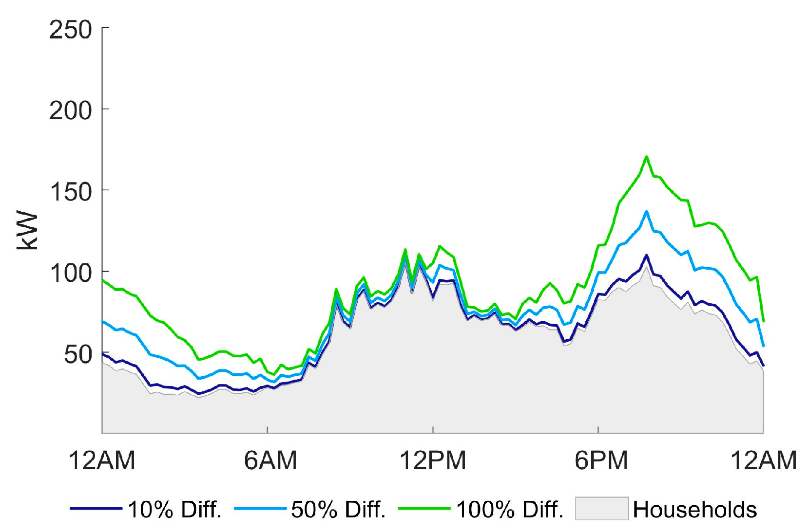
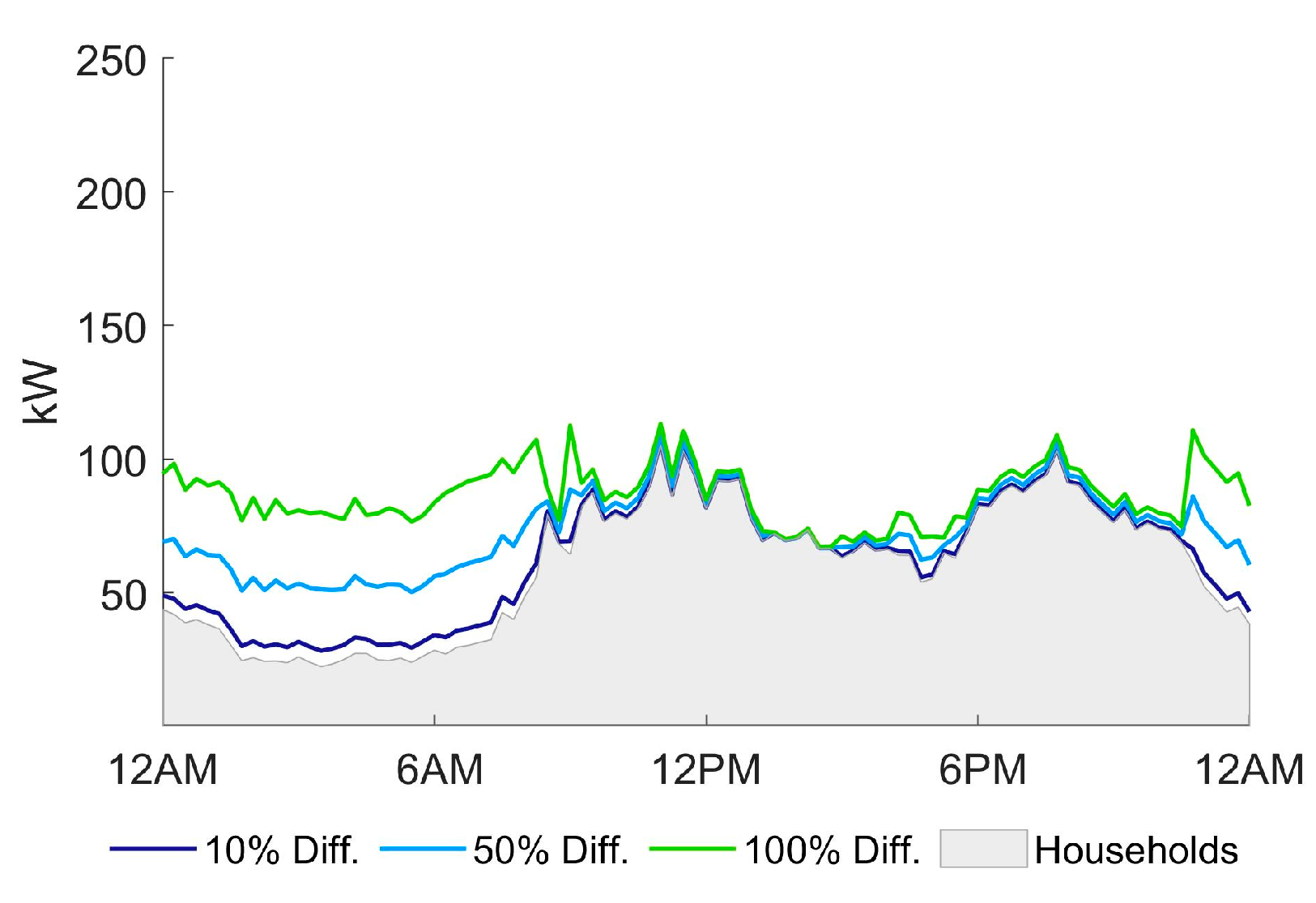
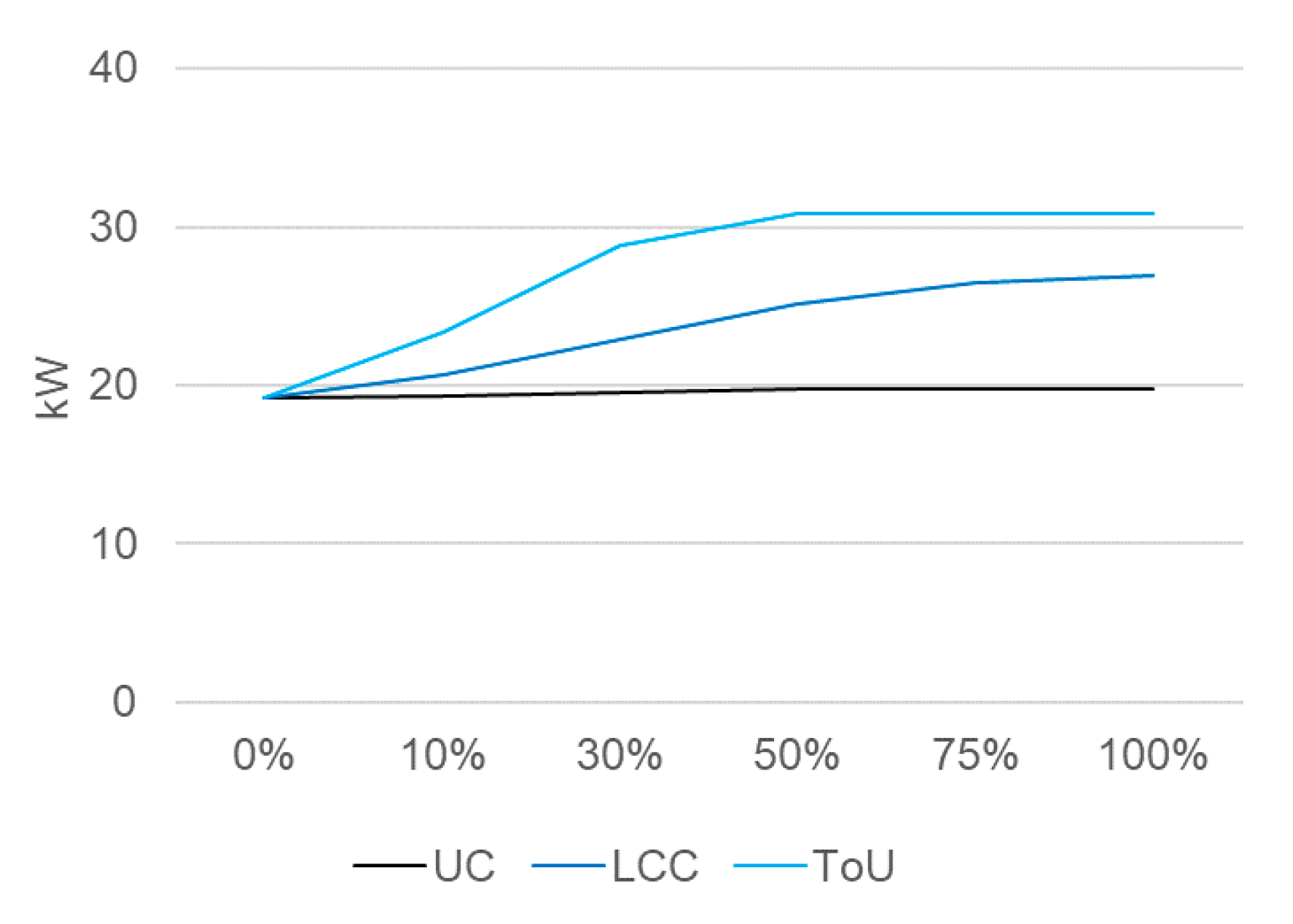
Compared to uncontrolled charging, where BEV charging coincides with a higher HH electricity demand, the LCC approach operates at a slower charging speed, leading to an extension of charging times into the load valleys. The most successful load shift into the valleys is obviously achieved by the ToU approach, which is based around this exact objective (see Figure 14). While the demand minimum does not change through e-mobility in the uncontrolled charging scenario, it increases by 7.5% with the ToU approach. 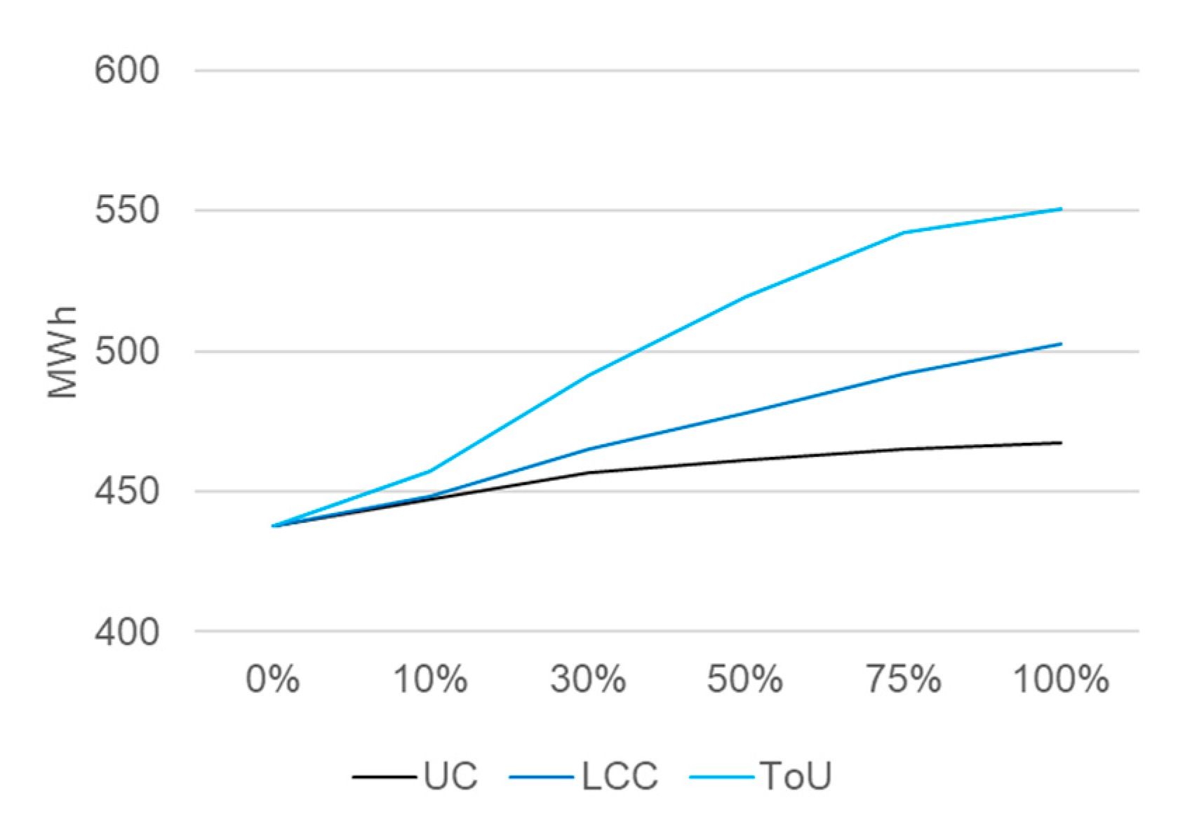Similar developments can be observed for the base volume demand below the P70 threshold (see Figure 15). With uncontrolled charging increasing the base volume demand by 20% toward full BEV diffusion, the LCC approach already leads to an increase of 42%. The aim of the ToU approach to avoid HH load peaks and shift the demand into the base volume represents the most successful load shifting measure. As a result, the base volume demand increases substantially under this LM strategy up to 551 kWh—a 74% increase compared to no e-mobility.

If the value of a ToU approach is compared to the situation under uncontrolled charging between 10% and 100% BEV diffusion, we discover a 10–40% reduction in the maximum demand and a 17–39% reduction in the peak volume demand. Toward full BEV diffusion, the minimum demand rises by 56% with the ToU approach, and the base volume demand increases by 18% compared to uncontrolled charging. This is the result of effective load shifting away from existing HH peaks into valleys. These results represent a substantial reduction in the maximum and peak volume demands caused by E-mobility and, therefore, they could have significant value related to the sufficiency of the local power connection, distribution grid performance, and the prevention of IS expansion requirements.

This highlights the importance of LM for the further development of charging solutions. At the same time, fears of the impact of E-mobility on these aspects or skepticism for the sufficient availability of charging points in nearby public or, ideally, private environments is often a reason not to switch from conventional cars to this more environmentally friendly alternative. Therefore, we claim that proving the ability to control BEV electricity consumption may help legitimate such solutions in urban, multi-apartment buildings—a decision that needs to be made by the facility owner—and also promote the acceptance of e-mobility among potential users. Thus, overall, the availability of solutions for large-scale charging IS may contribute to the goal of zero-emission mobility.

4.2. Verification with Results from Project Demonstration Phase

The demonstration phase of the Urcharge project tested extensions of the LM algorithm over 6 months in a residential area with 50% e-mobility, where 27 BEVs were controlled with LM and 24 were charging uncontrolled. The project mostly included BEVs of the type Renault Zoe, a few Nissan Leaf, and two Tesla models. Mode 3 charging points with Type 2 chargers were used. Additionally, the customer perspective was analyzed with surveys and interviews among the participants. In this real environment, the basic LM approach, which is enhanced by specific technical functionalities, involves control over the charging capacity across all or single charging stations to avoid exceeding the building’s available power connection. Therefore, the charging processes of single vehicles are only interrupted or postponed when the current defined capacity is reached. This largely represents the LCC approach of our model (see Section 2.3.1). However, the modeled environment cannot fully depict the reality of the relevant technical functionalities. The main differences are described in

Table 4. Differences between the modeled and the real environment.

No.	Topic	Model	Demo Phase
1	Information on energy consumption and BEV charging availability	Full information for LM optimization (Section 3.3) Comparison between full and daily information for minimum charging capacity (Section 3.4)	No information
2	Battery state of charge	Known	Unknown
3	Ratio plugged in/time parked	100%, always plugged in when parked	45% of the time plugged in when parked
4	Ratio plugged in/charging	Charging takes place during 30% of the plug-in time for uncontrolled and 47% for ToU charging	Charging takes place during 50% of the plug-in time
5	BEV share analyzed	0–100%	50%
6	LM	Constraints according to charging strategies in Section 2.3.1. ToU based on HH electricity demand	Charging as a system totally separate from the HH load. However, the HH load should be guaranteed. If BEV charging exceeds the building’s power connection, charging is stopped first.
7	Phase charging	Each charging point provides 3.7 kW for charging.	1 or 3 phase charging: 1 phase vehicles currently always block all 3 phases with 11 kW but only consume 3.7 (11/3) kW. The LM algorithm was further developed in this project to release the available 2 phases to other 1- or 2-phase BEVs. In the future, this will release a substantial amount of capacity.

.

Extrapolated to one year, the average distance traveled during the demonstration phase by the project participants would be 11.100 km, which is slightly below the average of big cities in Austria (except Vienna) of 12.237 km/a [50]. The analysis of customer perspective within the project, carried out through surveys, revealed that this result could be due to the Covid-19 restrictions on daily driving for purposes such as work, visits, and leisure. On the other hand, few have increased their driving to avoid crowds in public transport. The monitoring shows that with an increasing experience, the user reduces the frequency of charging at the private station due to increasing knowledge of the BEV’s charging requirements. The average user plugs in every fourth day for about 14 h. The overall charging time ratio related to the total plug-in time in the demonstration phase is 50%, whereas the plug in to parked time ratio is about 45%. This results in a charging time ratio related to the parking time of 22.5%. Our model has an average charging to plug-in time ratio of 9% with uncontrolled and 15% with ToU charging, which can be explained by the fact that the BEVs are always assumed to be plugged in while parked (100%). In our model, sometimes, all BEVs are charging at the same time. However, on average, the uncontrolled scenario leads to 50% of simultaneous charging and the LCC approach leads to 86%. The project’s demonstration phase showed significantly lower simultaneity and charging time. At maximum, 12 BEVs were plugged in at the same time, which represents 44% of all BEVs, and a maximum of 11 BEVs were charging at the same time (41%). The average results were 24% and only 12%, respectively.

Of course, this is a major difference to our model parameters in which all BEVs are assumed to be available and plugged in at the charging point during any time while parked at home. The average amount of energy consumed during each charging session and BEV is 22 kWh. The plug-in times are mostly focused between 5 and 7 pm, whereas plug-out times typically range between 6 and 7 am. This fact supports the assumption of high flexibility due to long charging periods in private networks. Public charging is used very rarely.

Despite the assumptions in the modeled environment, the conclusions from the project’s real environment support the findings in this study. To test the capabilities of the LM functions and the minimum required charging capacity to guarantee the fulfillment of the BEV charging demand, during the demonstration phase, the available charging capacity was reduced several times from 35 kW for 27 BEVs (1.3 kW/BEV) down to 25 kW (0.9 kW/BEV). Therefore, the required charging capacity across all charging points could be reduced below the expected level of about 1 kW/BEV, and critical situations with respect to the power connection capacity would not occur. This matches our analysis provided in Section 3.4 of the minimum charging capacity, which can have a significant impact on the cost of charging infrastructure.

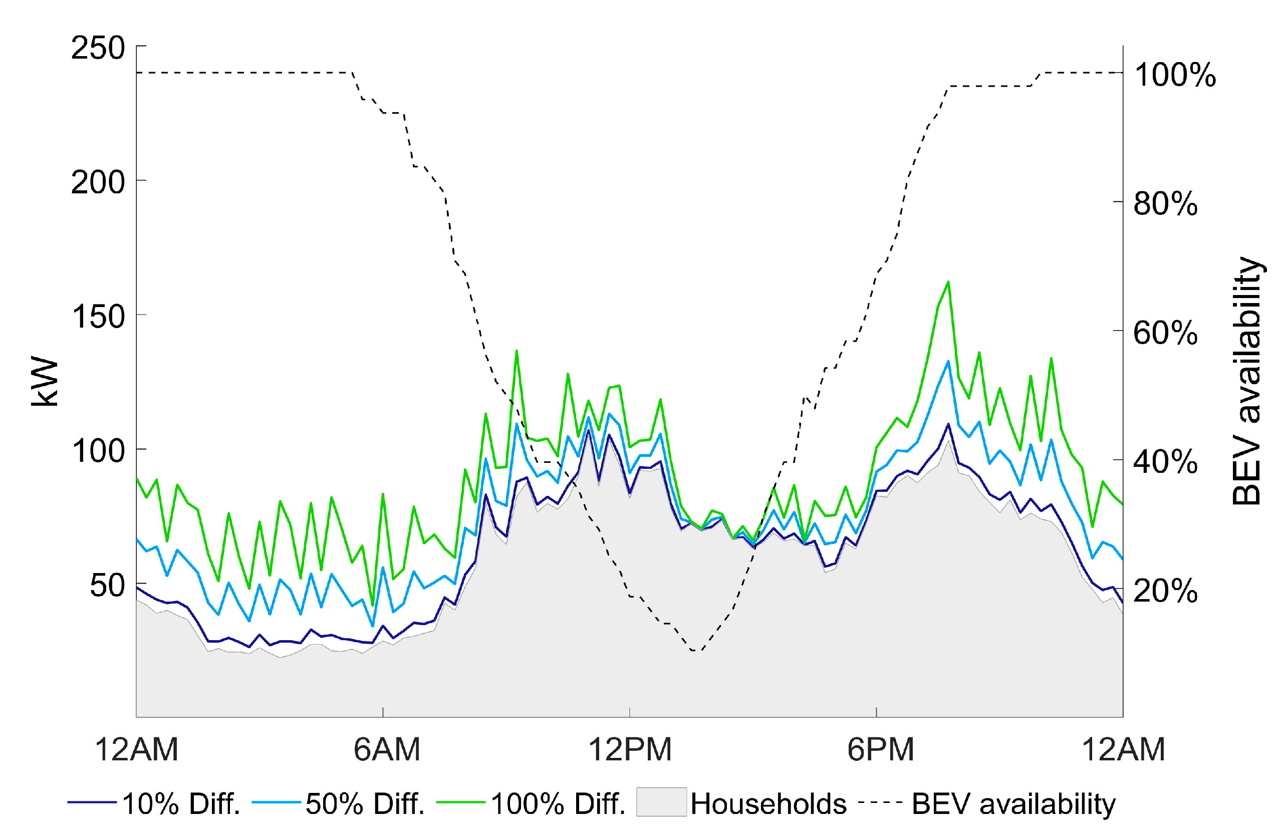
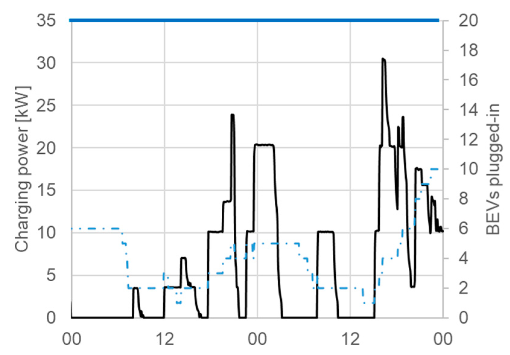
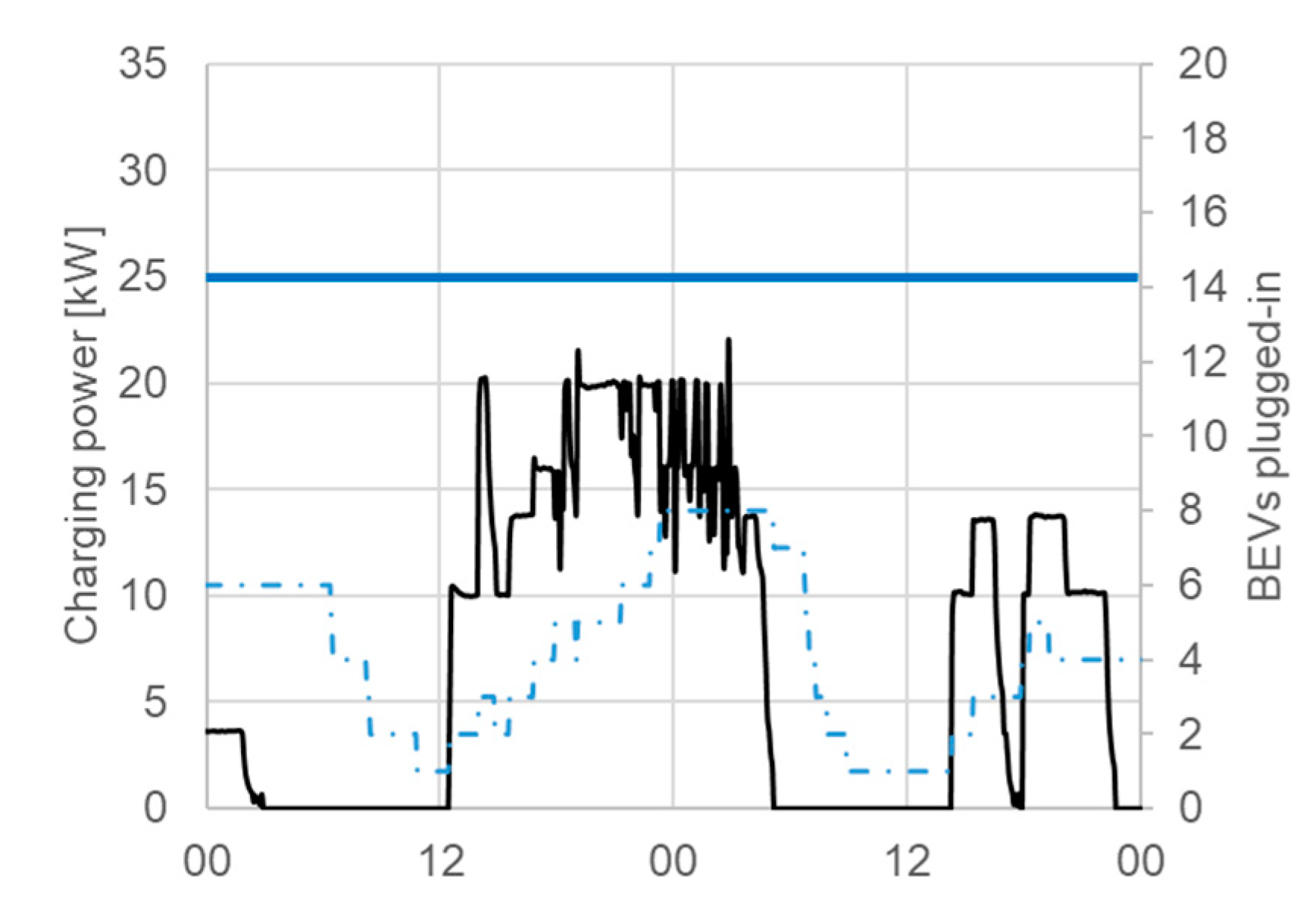
Figure 16 shows the BEV charging power with an overall initial charging capacity of 35 kW together with the number of cars currently plugged in. In this exemplary period, 31 kW was reached once during the evening, resulting in a significant impact of e-mobility on the overall building load. On the other hand, Figure 17 shows the situation with a reduced overall charging capacity down to 25 kW, which results in longer charging periods and significantly limits the electricity demand peaks. Furthermore, the dependence on the availability of BEVs plugged in at the charging station, which only accounted for 45% of the parking time in this project, becomes more important under this situation, since charging operates much slower. The project experience also revealed that a higher share of plug-in times would improve LM efficiency. In the first week with 1.3 kW/BEV of charging capacity, the building’s electricity demand maximum (HH + BEV) increased almost twofold due to e-mobility. Later, with a reduction down to 0.9 kW/BEV, the LM successfully operated below this threshold, which reduced this surge.

The users recognized little reduction in charging performance under a reduced capacity. From the demonstration phase findings, it can be expected that LM will enable the coordination of 100% e-mobility in the residential area with sufficient comfort for the users and without any impact on the distribution grid capacity. Our model, as calculated in Section 3.4, determined a minimum charging capacity of 0.44 kW/BEV under a scenario with full information and 1.3 kW/BEV with a daily rolling approach, roughly matching the threshold tested in the demonstration phase. With the phase-dependent charging currently being developed and tested, as explained in line 6 of Table 4, the capacity gains will lead to more efficient LM in this respect.

4.3. Environmental Aspects of E-Mobility and Advantages of LM

This section discusses the results for the environmental effects of e-mobility, as well as the advantages through LM and the efficient sizing of charging capacity. Of course, all the considerations for minimization of the capacity requirements have not only environmental but also economic aspects.

• Savings in GHG emissions from the substitution of conventional vehicles with BEVs

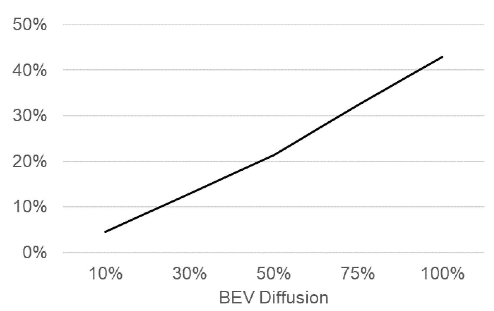
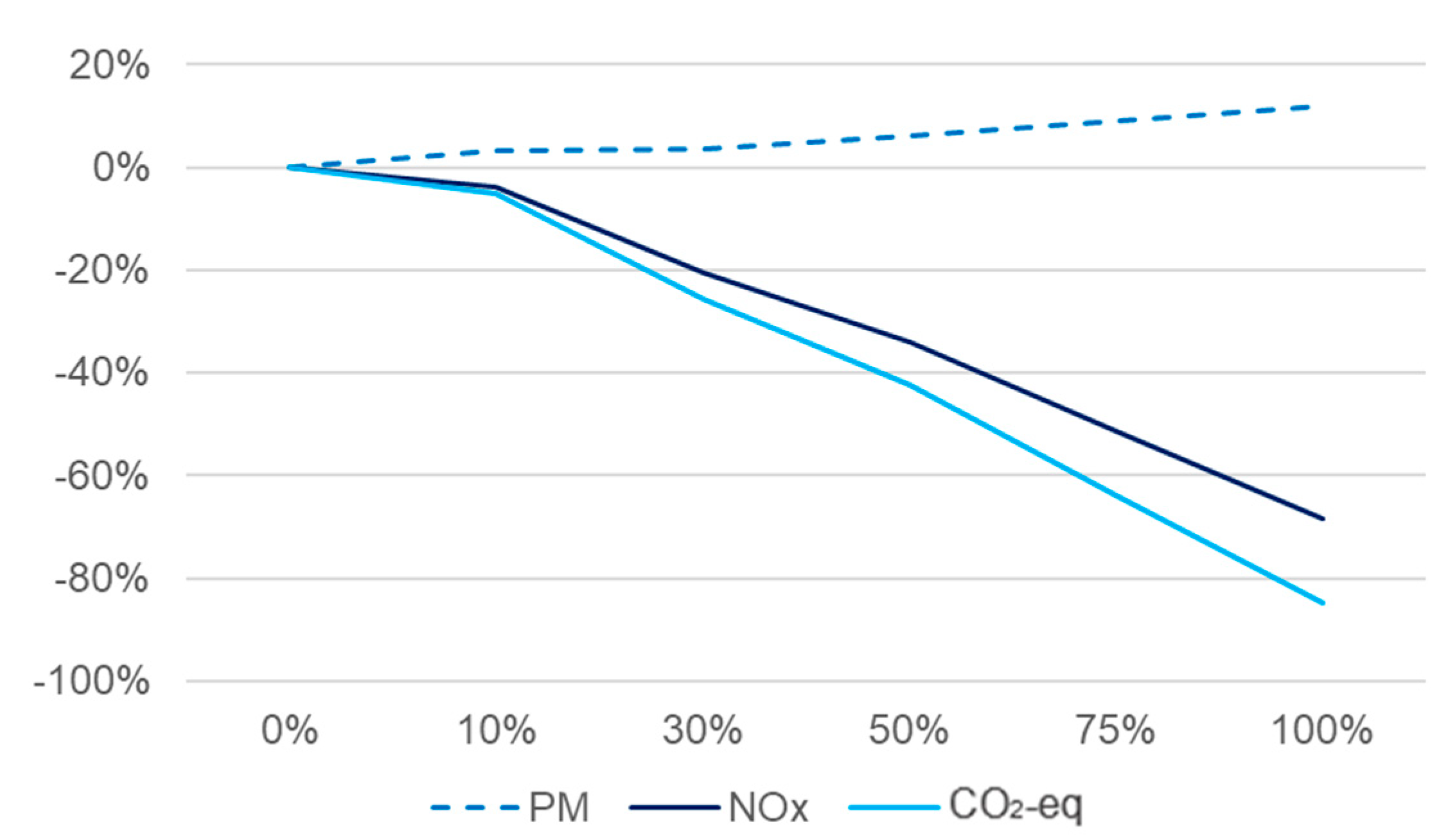
In the considered residential area, e-mobility accounts for an increase in the yearly electricity consumption of 13% with a 30% BEV share and 43% with full BEV diffusion, as shown in Figure 18. According to our methodology, the development of the yearly CO₂-eq and NOx emissions, as well as particulate matter (PM), under the substitution of conventional cars with BEVs is shown in Figure 19.

All conventional cars in the residential area, considering an Austrian mix of diesel- and petrol-powered engines, emit 268 tCO₂-eq/a. By 2030, Austria aims at a BEV share of 30% representing a substitution of 32 conventional cars with BEVs in the residential area. This would result in 26% savings in yearly CO₂-eq emissions, accounting for 12 tCO₂-eq and 21% NOx savings by 2030. However, according to the UBA [52], during their life cycles, BEVs emit more PM than diesel- or petrol-powered combustion engines due to the emissions caused during vehicle and battery construction. This would lead to a 4% increase in PM emissions for 30% BEV diffusion. The overall 2030 goal in Austria is a 36% reduction of CO₂ emissions in transport [55]. Considering the aim of increasing the use and decarbonization of public transport, this goal may be achievable if the diffusion of BEVs can be realized as planned.

2.

Impact of LM on the environmental aspects of the electricity mix consumed for charging

Our model provides evidence on the negative environmental impact of electricity demand increases with respect to the electricity mix consumed at least from the correlation coefficient between BEV charging and fossil electricity generation ($r_{\mathrm{foss}}$). Whereas uncontrolled charging shows a very weak positive correlation with 0.10 according to Pearson [57], the ToU approach results in a weak negative correlation of −0.24 and therefore seems to increase the use of renewable energy sources.

Furthermore, an analysis of the Austrian national electricity demand and the amount of national fossil power generation (coal and gas) in 2019 revealed a strong positive correlation between the two of 0.65. Additionally, an average HH load profile shows a moderate correlation with the overall national load profile of 0.49. Therefore, we claim that an increase in the building’s electricity demand peaks due to e-mobility, such as with uncontrolled charging, leads to a negative environmental impact on the electricity mix consumed. LM can control the distribution of charging power to reduce the consumption of fossil fuel electricity generation during demand peaks.

3.

Environmental impact of E-mobility and LM on potential grid expansion

The electricity demand profile of BEVs has a widespread impact on the cost and environmental effects related to the required capacity of power connection, the distribution grid, and even electricity generation capacities.

A reduction in electricity demand peaks through LM can guarantee the sufficiency of existing distribution grid capacities and thereby obviate the need for expansion investments [16]. Additionally, short-term peaks, apart from the described impacts on the electricity mix and use of flexible fossil power plants, would have an effect on the installed electricity generation capacities. A greater distribution of the overall electricity demand would yield a flatter demand profile and avoid the significant investment costs, as well as the associated resource consumption, land-use, and emissions from component production.

5. Conclusions

Firstly, our modeling results prove that uncontrolled charging results in a correlation between BEV electricity demand and HH load peaks. This results in a negative impact of growing e-mobility on distribution grid performance, as well as a negative impact on the environmental aspect of the electricity mix consumed while charging. Ou that LM is an important solution to control BEV charging demands and reduce this impact. Under full information, with between 10% and 100% BEV diffusion, an off-peak ToU approach can achieve a reduction in the building’s maximum electricity demand between 10% and 40% compared to uncontrolled charging. The peak volume demand—the sum of the demand exceeding a certain threshold—can be reduced between 17% and 39%. This is partly achieved by a time shift of charging into valleys and by a reduction in the charging power consumed and an associated increase in the charging time periods. As a result, the electricity demand that is shifted from the HH load peaks fills up the load valleys and increases the former demand minimum. This may result in a modification of known building electricity demand profiles. On the one hand, these profiles could become more even due to the valleys being filled. On the other hand, increasing the electrification of a growing amount of applications could result in additional (or new) peaks in the future.

Our study reveals the value of information on user behavior and BEV energy consumption for LM efficiency. In this study, we calculated the minimum size of the charging capacity required to fulfill the BEV electricity demands in a private charging network. In a yearly optimization model with full information and under the assumption that parked BEVs are also plugged in, the minimum charging capacity is 0.44 kW/BEV. Less information in a daily rolling optimization leads to an almost threefold capacity requirement of about 1.3 kW/BEV. The Urcharge demonstration phase revealed that the average user plugs in for charging only every fourth day, reducing the flexibility of LM in a real environment. In reality, future BEV energy consumption and plug-in times are unknown. Nevertheless, the charging capacity in the demonstration phase could be decreased to 0.9 kW/BEV, thereby cutting the demand peaks and reducing the impact on the distribution grid. This study clearly highlights the benefit of using more information to provide longer foresight and flexibility with higher predictability for upcoming BEV charging demands.

One way for an electricity provider to collect users’ behavioral information and charging preferences is via a mobile app. Currently, because the battery’s state of charge remains unknown to the master station, electricity providers could assign pre-defined charging profiles to single charging points or groups aligned with the user’s preferences communicated via an app (charging deadlines, day/night charging, etc.). Efficient LM and charging capacity sizing also have significant positive environmental effects. While 100% E-mobility increases yearly electricity demands in the residential area by 43%, the substitution of fossil-fuel-powered vehicles results in significant reductions in CO₂-eq and NOx emissions over a vehicle’s lifecycle. Interestingly, off-peak charging can achieve a negative correlation between fossil fuel electricity generation and BEV electricity consumption, thereby promoting the use of renewable energy sources. Without an increase in peak demand through e-mobility and efficiently sized private charging capacity, not only could the expansion of the distribution grid and power generation capacities be avoided, but the emissions associated with the electricity mix consumed could also be controlled.

In general, our work proves the ability of LM in multi-apartment buildings to solve most of the common challenges associated with distribution grid performance throughout growing BEV diffusion. The implementation of this controlled, large-scale, and private charging IS offers vast economic, technical, and environmental advantages compared to more isolated and uncontrolled solutions. First, a private charging network offers substantial advantages for LM due to the high availability of the BEVs at the charging station and the lower time-criticality of charging. Secondly, LM avoids an increase in electricity demand peaks and thus prevents distribution grid expansion and the use of thermal power generation. As a result, the total cost of BEV charging, as well as the environmental impacts, can be managed. In the future, for the benefit of the whole energy system in terms of costs and environmental effects, regulatory and market frameworks need to be established to promote the implementation of a charging IS that applies controlled, joint solutions rather than isolated, fast charging options. LM could be enhanced by research on forecasting the relevant parameters, such as weather and traffic conditions, and the optimal integration of renewable energy. Eventually, BEV charging needs to be integrated into an overall system perspective. These are the next steps for future research and development.