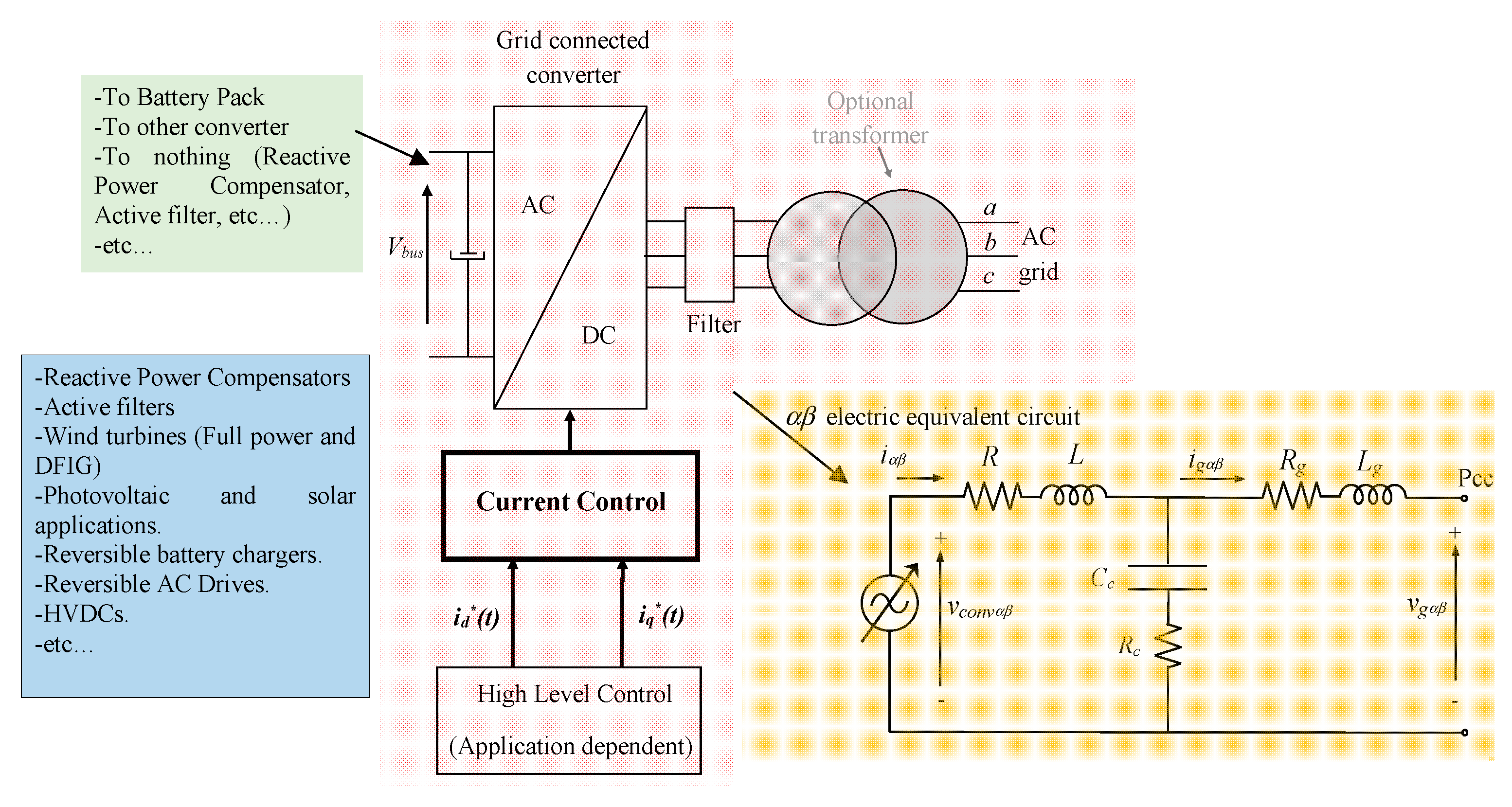
Figure 1.
Grid-connected converter operating with current references in the dq reference frame; id*(t) and iq*(t) and simplified equivalent electric circuit in the αβ reference frame.
Figure 1.
Grid-connected converter operating with current references in the dq reference frame; id*(t) and iq*(t) and simplified equivalent electric circuit in the αβ reference frame.
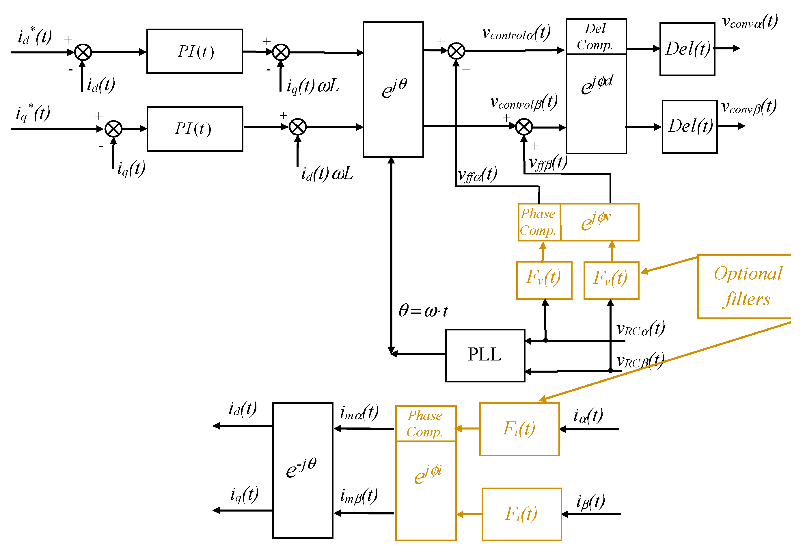
Figure 2.
Fundamental current control loops using PI regulators in the dq reference frame.
Figure 2.
Fundamental current control loops using PI regulators in the dq reference frame.
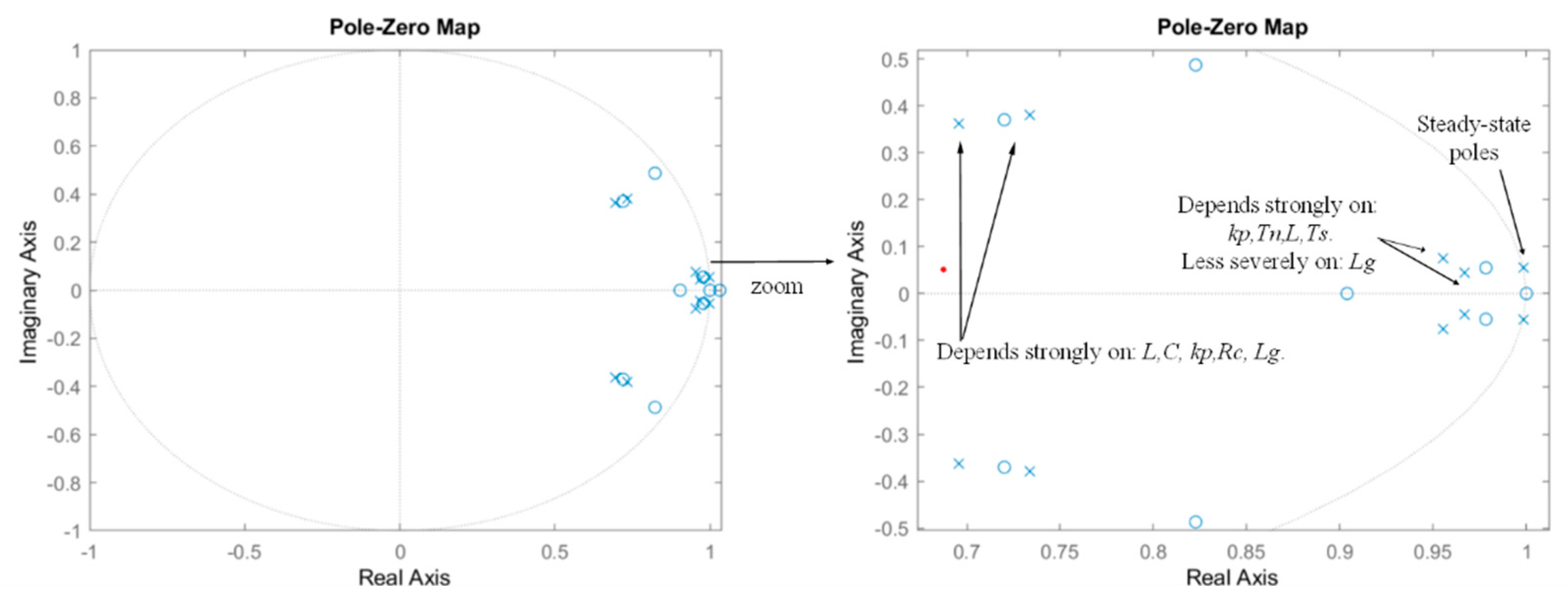
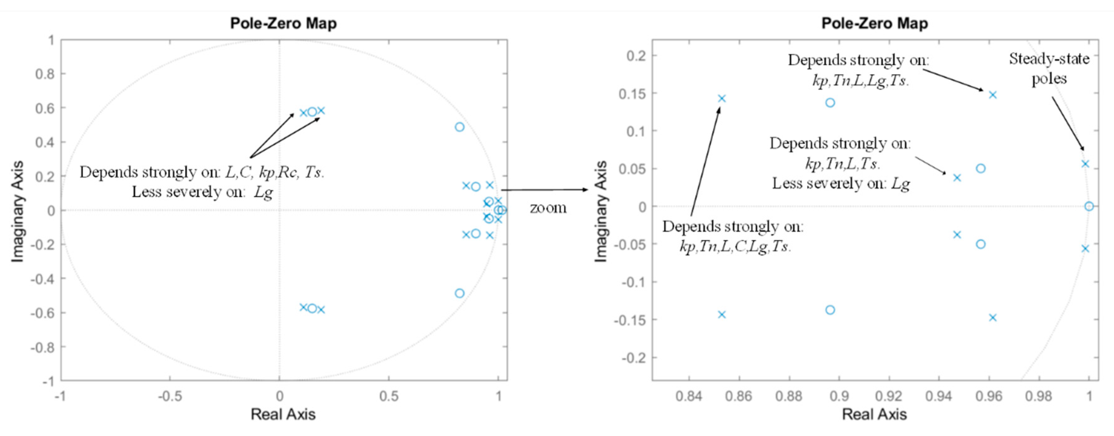
Figure 3.
Poles and zeros of
iα(
z)
/id*(
z) and dependence on the parameters in the
αβ reference frame for step input references, corresponding to the control of
Figure 2, deduced from the mathematical model of
Table 1, and applied to the numerical scenario of
Appendix A. The voltage and current filters are not included, and it is assumed that there is no delay in the converter voltage update, i.e.,
Fi(
z)
= 1,
Fv(
z)
= 1,
Del(
z)
= 1 and
ϕi = ϕv = ϕd = 0. The poles for the rest of the controlled input–output relations are equal (
iα(
z)
/iq*(
z),
iβ(
z)
/id*(
z),
iβ(
z)
/iq*(
z)).
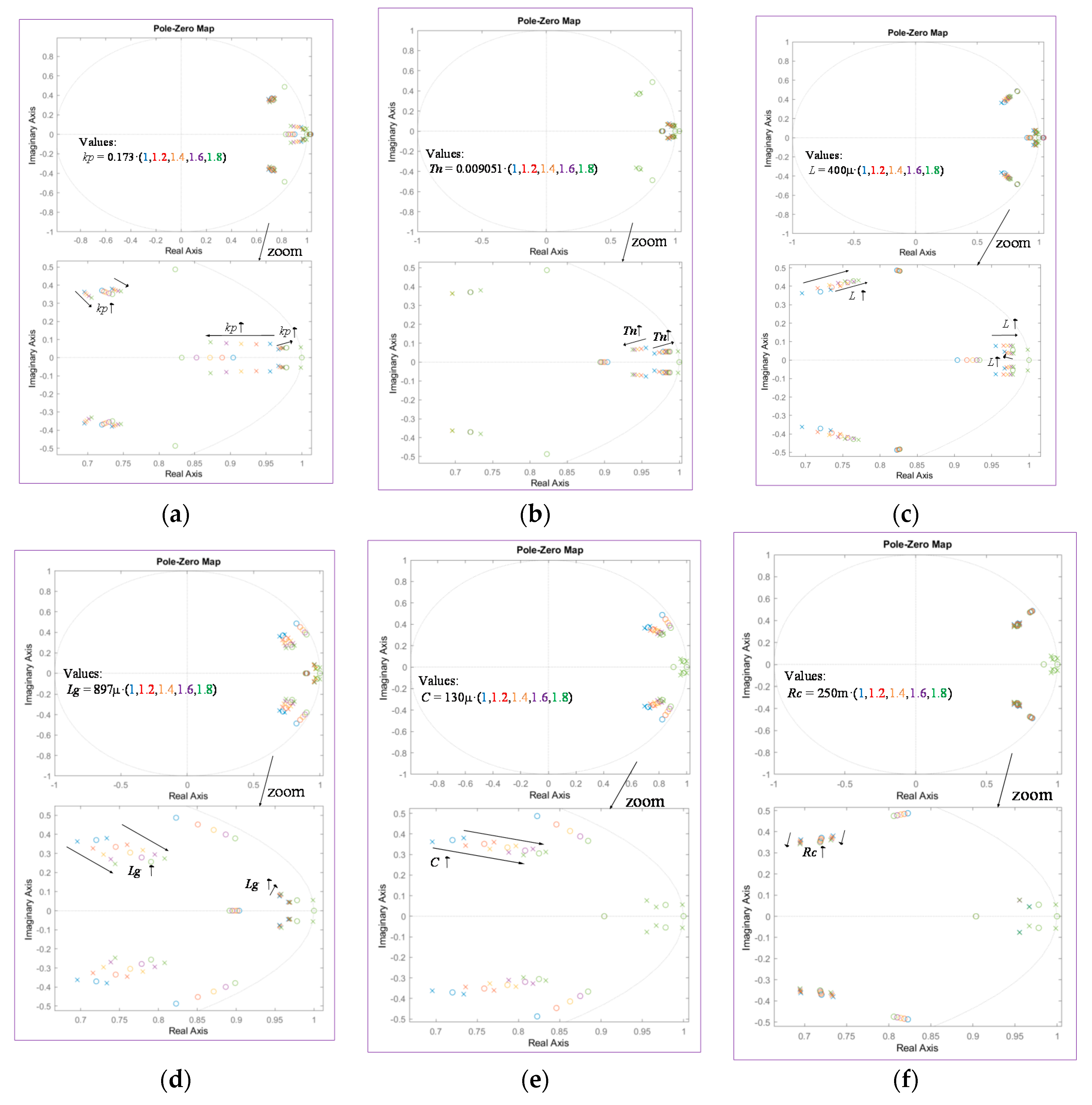
Figure 4.
Variation of the poles and zeros of
iα(
z)
/id*(
z) in the
αβ reference frame for step input references, corresponding to the control of
Figure 2, deduced from the mathematical model of
Table 1, and applied to the numerical scenario of
Appendix A. Each parameter’s value is modified within a range. Voltage and current filters are not included, and it is assumed that there is no delay in the converter voltage update, i.e.,
Fi(
z)
= 1,
Fv(
z)
= 1,
Del(
z)
= 1 and
ϕi = ϕv = ϕd = 0. (
a)
kp variation; (
b)
Tn variation; (
c)
L variation; (
d)
Lg variation; (
e)
C variation; (
f)
Rc variation.
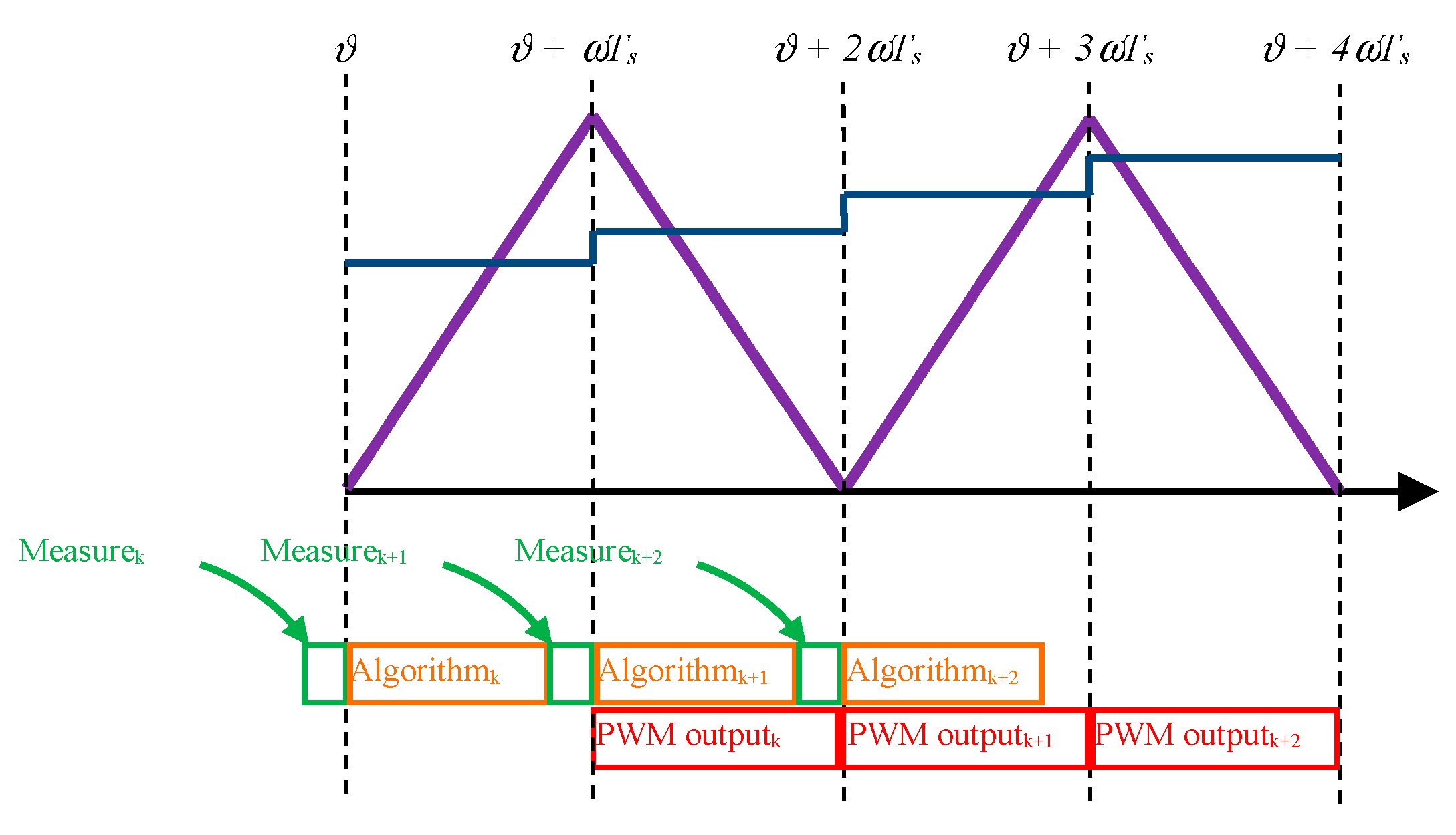
Figure 5.
Voltage modulation process with a classical asymmetrical regular sampled PWM, for one half bridge of the converter and resulting constant update delay of one sample time.
Figure 5.
Voltage modulation process with a classical asymmetrical regular sampled PWM, for one half bridge of the converter and resulting constant update delay of one sample time.
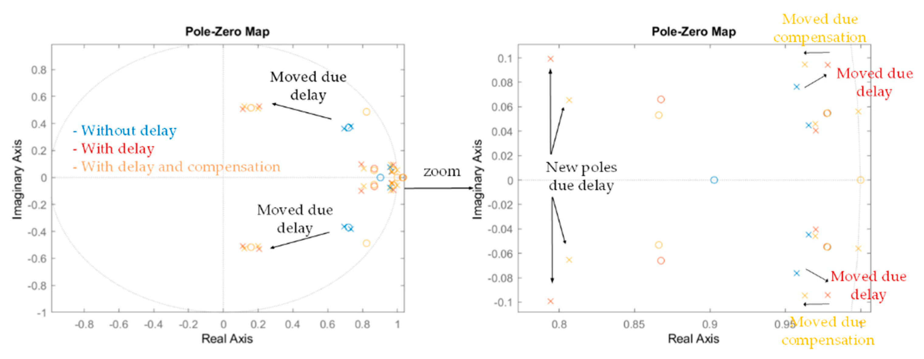
Figure 6.
Poles and zeros of
iα(
z)
/id*(
z) in the
αβ reference frame for step input references, corresponding to the control of
Figure 2, deduced from the mathematical model of
Table 1, and applied to the numerical scenario of
Appendix A. The voltage and current filters are not included, i.e.,
Fi(
z)
= 1,
Fv(
z)
= 1 and
ϕi = ϕv = 0. Blue: without delay, Red: with delay, Yellow: with delay and compensation. The poles for the rest of the controlled input–output relations are equal (
iα(
z)
/iq*(
z)
, iβ(
z)
/id*(
z)
, iβ(
z)
/iq*(
z)).
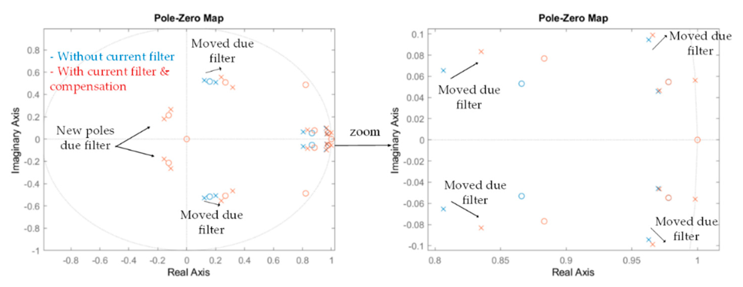
Figure 7.
Poles and zeros of
iα(
z)
/id*(
z)
, in the
αβ reference frame for step input references, corresponding to
Figure 2, deduced from the mathematical model of
Table 1, and applied to the numerical scenario of
Appendix A. The voltage filter is not included, i.e.,
Fv(
z) = 1 and
ϕi = 0. Blue: without current filter, Red: with current filter and its phase shift compensation at 50 Hz.
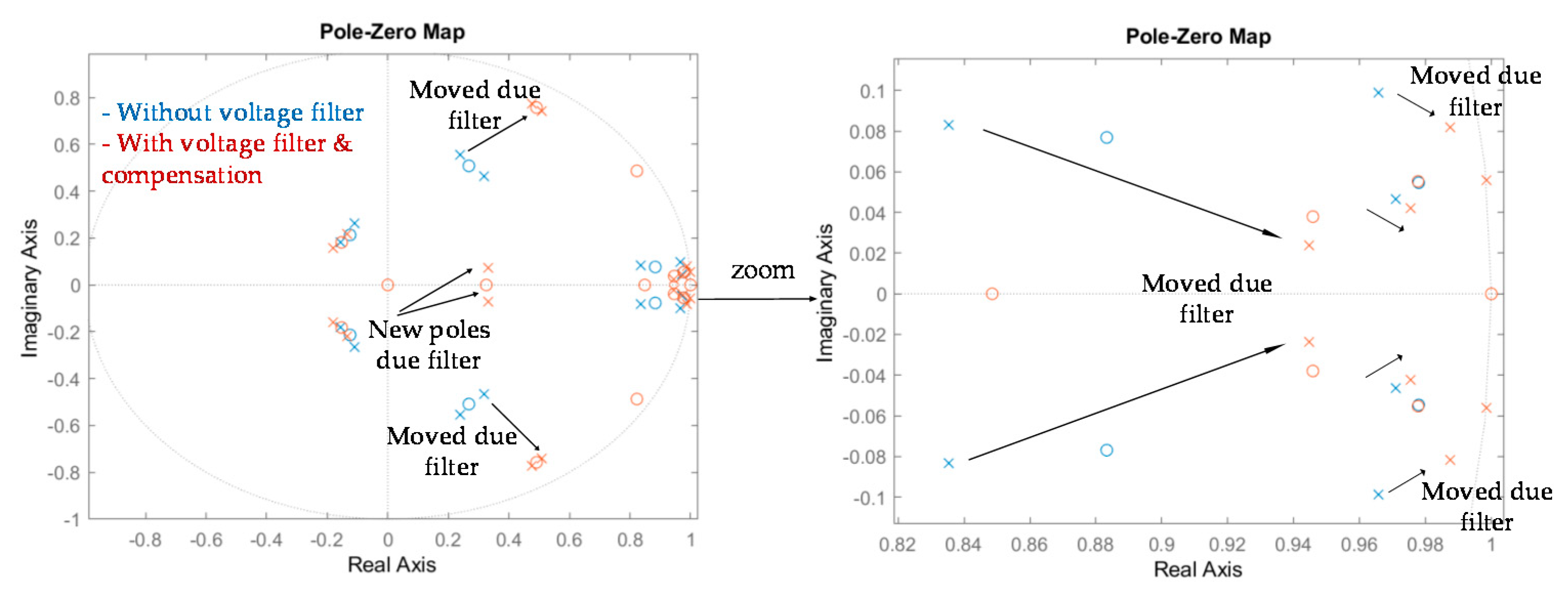
Figure 8.
Poles and zeros of
iα(
z)
/id*(
z) in the
αβ reference frame for step input references, corresponding to the control of
Figure 2, which is deduced from the mathematical model of
Table 1 and applied to the numerical scenario of
Appendix A. Blue: without voltage filter, Red: with voltage filter and its phase shift compensation at 50 Hz. The poles for the rest of the controlled input–output relations are equal (
iα(
z)
/iq*(
z),
iβ(
z)
/id*(
z),
iβ(
z)
/iq*(
z)).
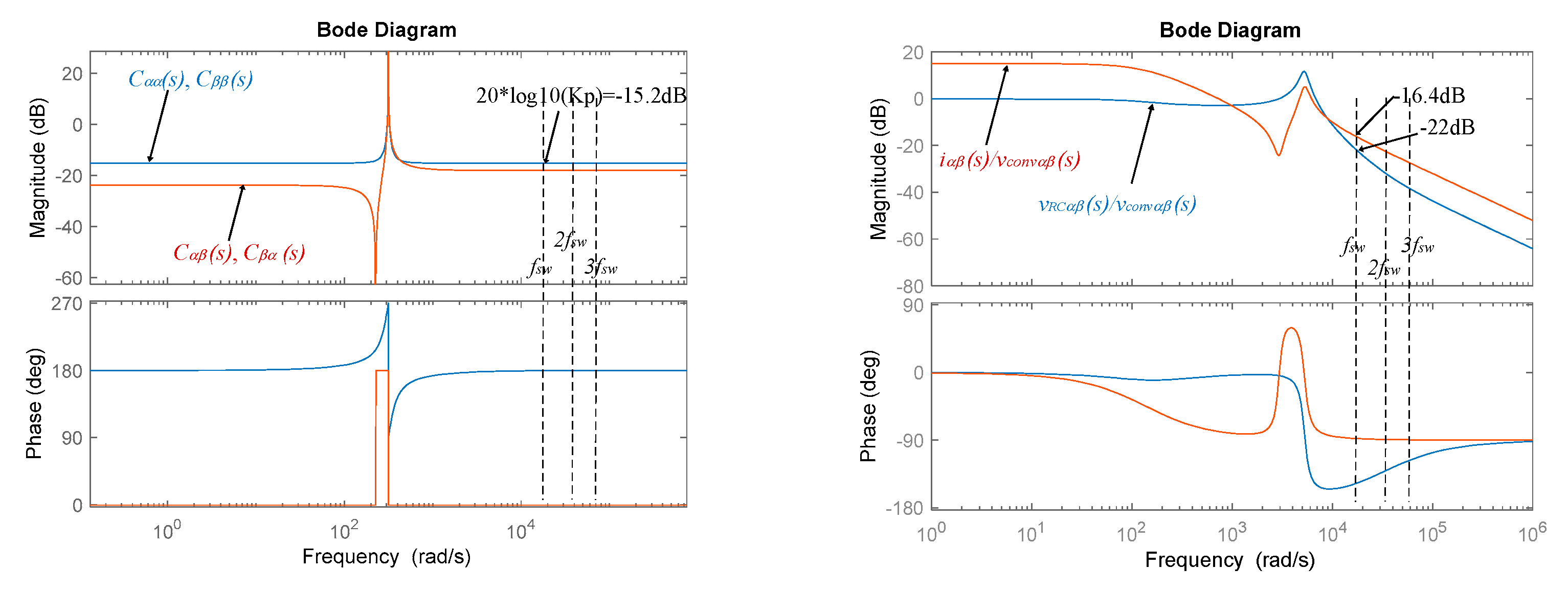
Figure 9.
Bode diagrams derived from the mathematical expressions involved on the ripple transmission from the voltage and current measurements and the output converter voltage generated by the control. Numerical values of
Appendix A.
Figure 9.
Bode diagrams derived from the mathematical expressions involved on the ripple transmission from the voltage and current measurements and the output converter voltage generated by the control. Numerical values of
Appendix A.
Figure 10.
Poles and zeros of
iα(
z)
/id*(
z)
, in the
αβ reference frame for step input references, corresponding to the control of
Figure 2, deduced from the mathematical model of
Table 1, and applied to the numerical scenario of
Appendix A. It is assumed that there is a delay in the converter voltage update, and the voltage and current filters are not included, i.e.,
Fi(
z)
= 1,
Fv(
z)
= 1. The poles for the rest of the controlled input–output relations are equal (
iα(
z)
/iq*(
z)
, iβ(
z)
/id*(
z)
, iβ(
z)
/iq*(
z)).
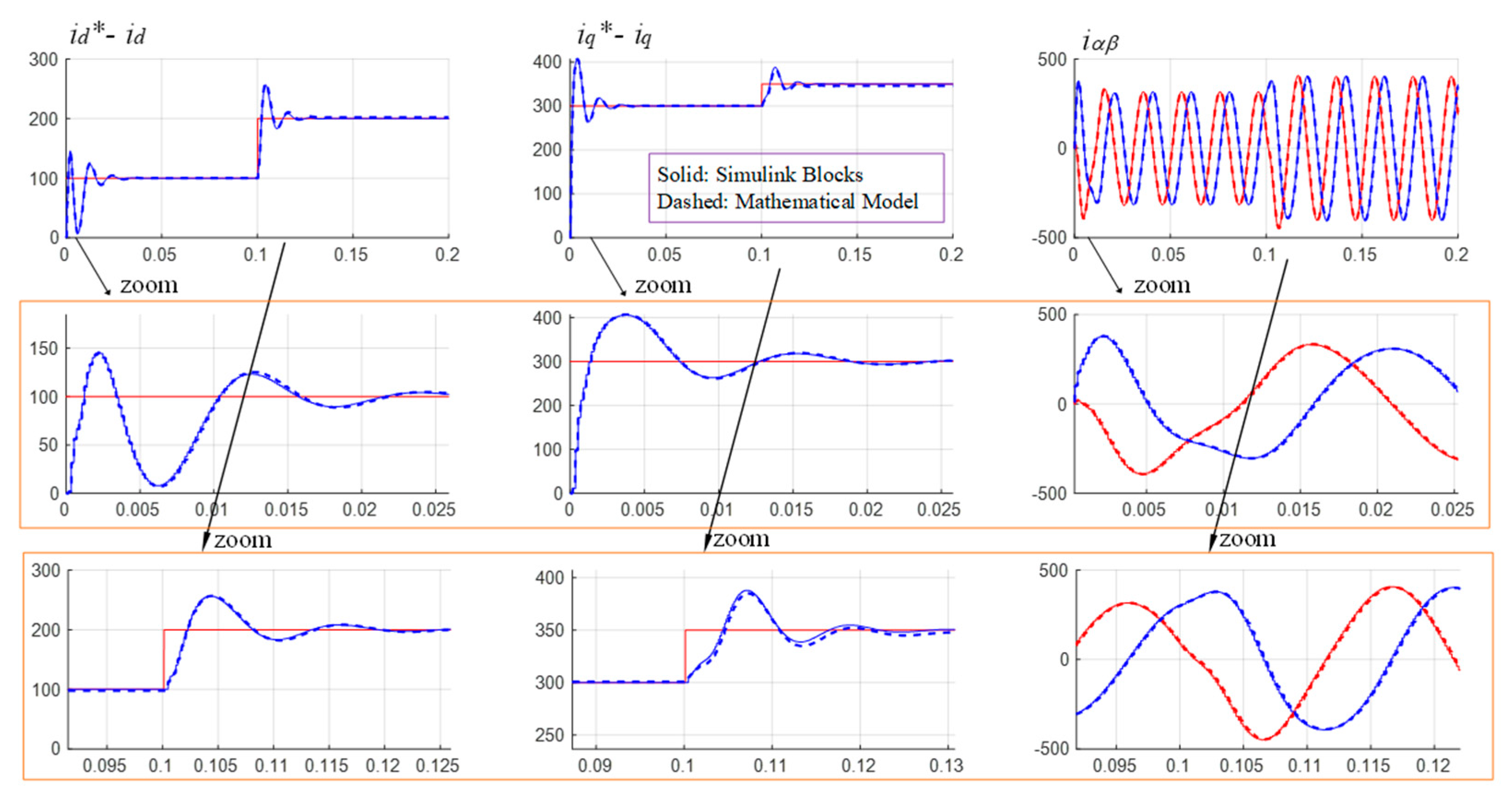
Figure 11.
Superposition of the time-domain responses of the mathematical model proposed in
Table 1 and the control block diagram of
Figure 2, built in Matlab-Simulink blocks by using ideal voltage sources as an ideal converter model. The same inputs and the same numerical parameters are used in both models (
Appendix A).
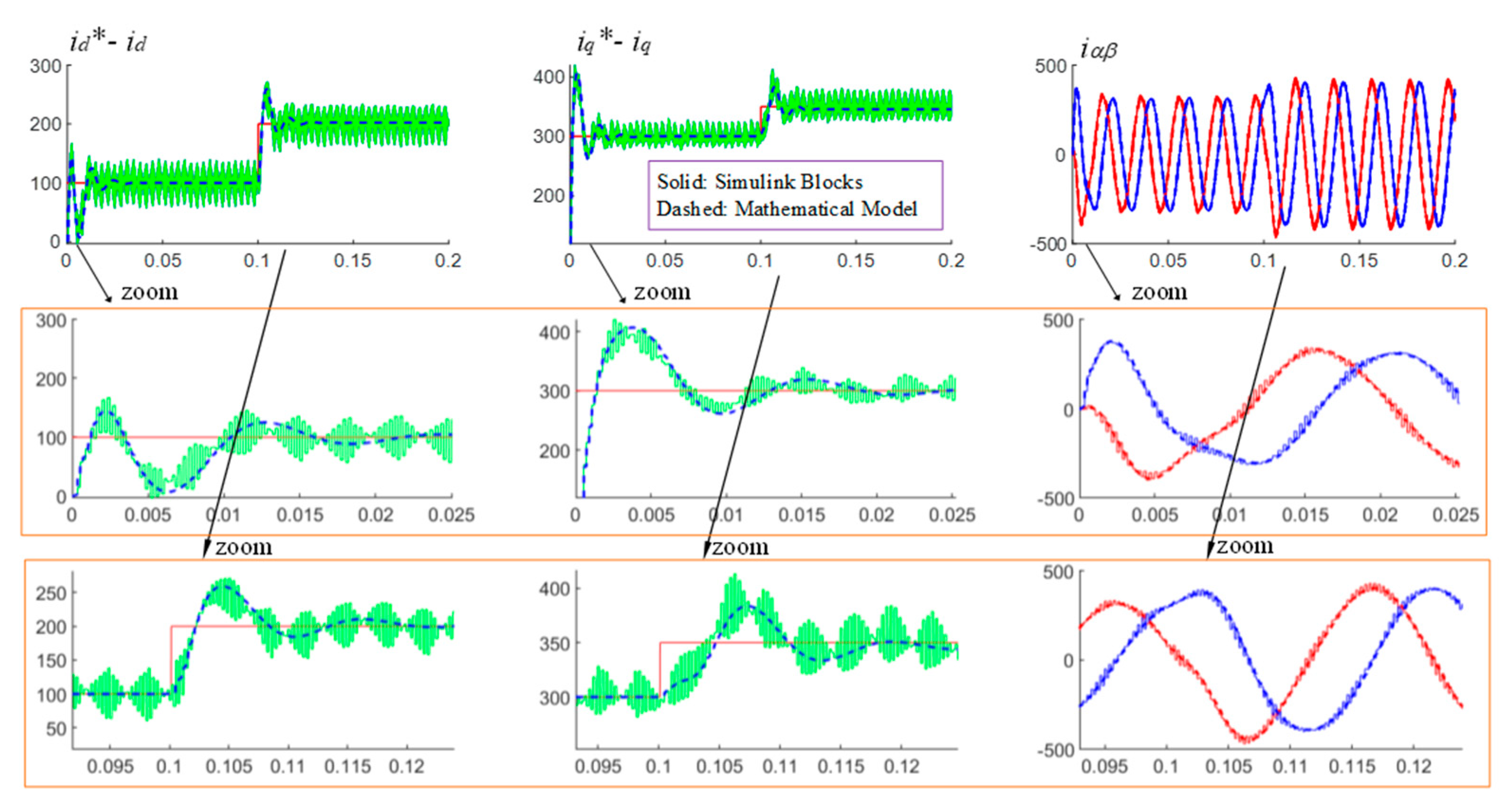
Figure 12.
Superposition of the time-domain responses of the mathematical model proposed in
Table 1 and the control block diagram of
Figure 2 (variables sampled at
Ts) built in Matlab-Simulink blocks by using a 3L-NPC (neutral point clamped) power electronic converter switched at fsw. The same input variables are applied at both controls, and the same numerical parameters are used in both models as well (
Appendix A).
Figure 13.
(
a) Superposition of the time-domain responses of the mathematical model proposed in
Table 1 and the correspondent experimental results. Same step input variables and same numerical parameters are used at both controls:
Lg = 0 mH, |
Vgrid| = 25 V, Pure inductive filter: R = 32 mΩ, L = 4 mH, Converter: 2L-VSC with IGBTs, switching at 8 kHz. (
b) A picture of the experimental platform.
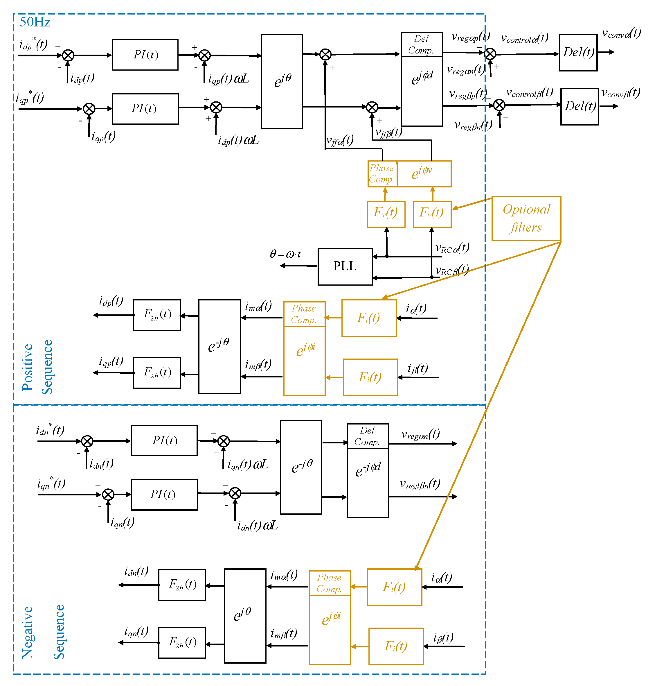
Figure 14.
Fundamental current control loops for positive and negative sequences using PI regulators in the dq reference frame: dual vector control.
Figure 14.
Fundamental current control loops for positive and negative sequences using PI regulators in the dq reference frame: dual vector control.
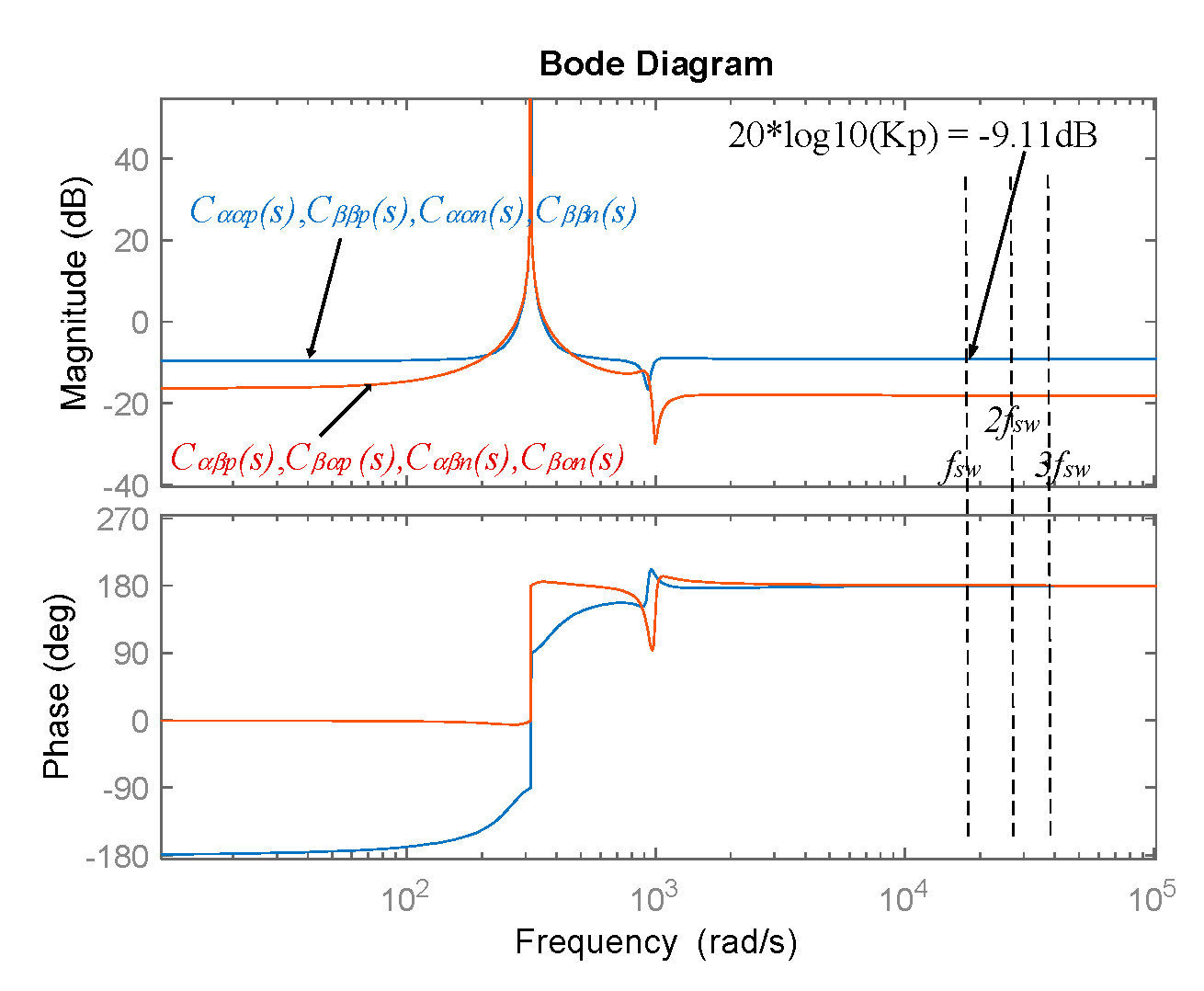
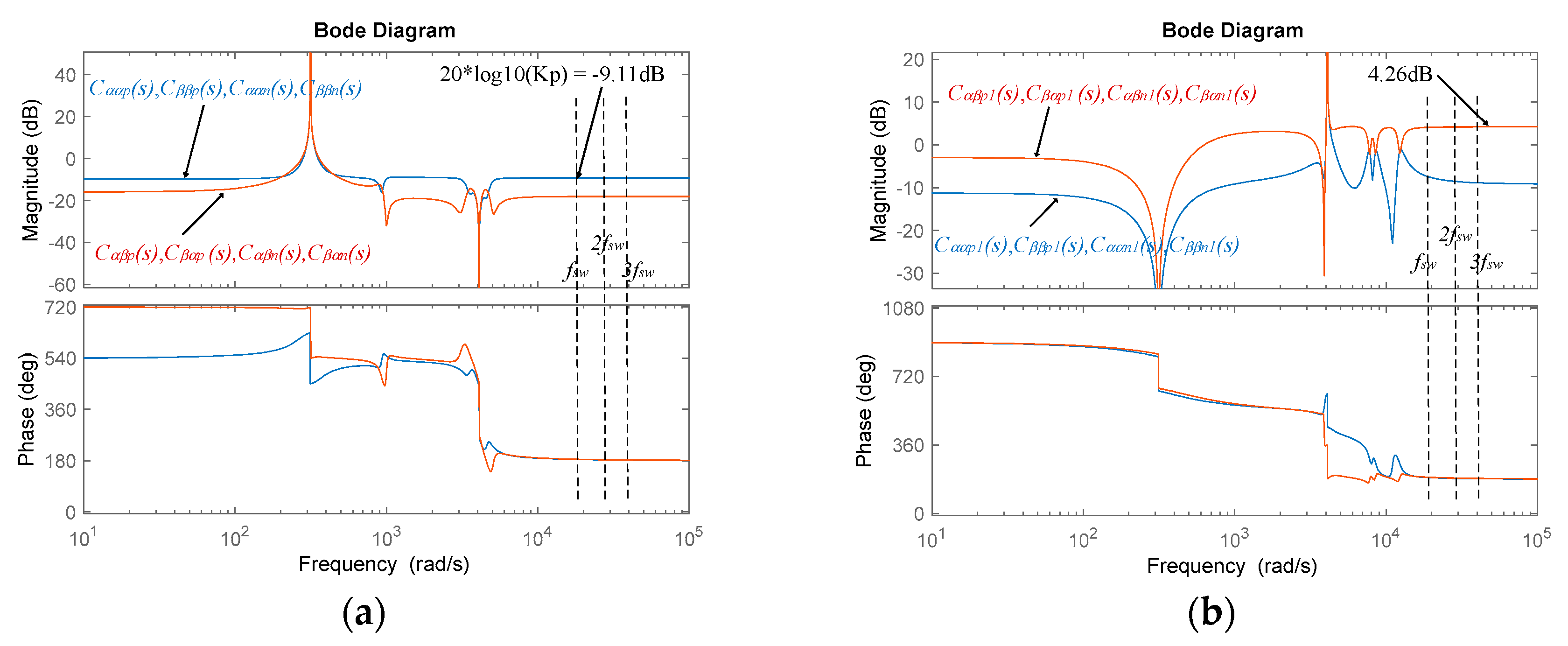
Figure 15.
Bode diagrams derived from the mathematical expressions involved on the ripple transmission; from the current measurements to the output voltage generated by the control. Numerical values of
Appendix B.
Figure 15.
Bode diagrams derived from the mathematical expressions involved on the ripple transmission; from the current measurements to the output voltage generated by the control. Numerical values of
Appendix B.
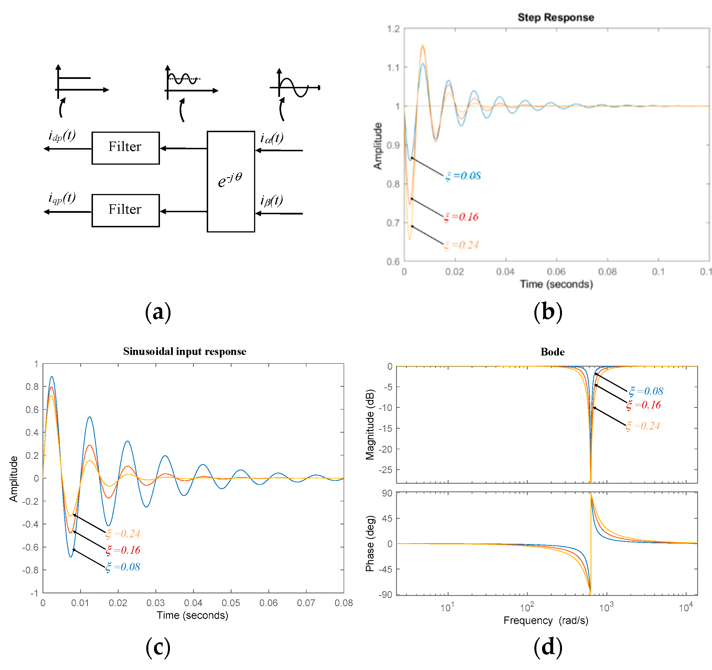
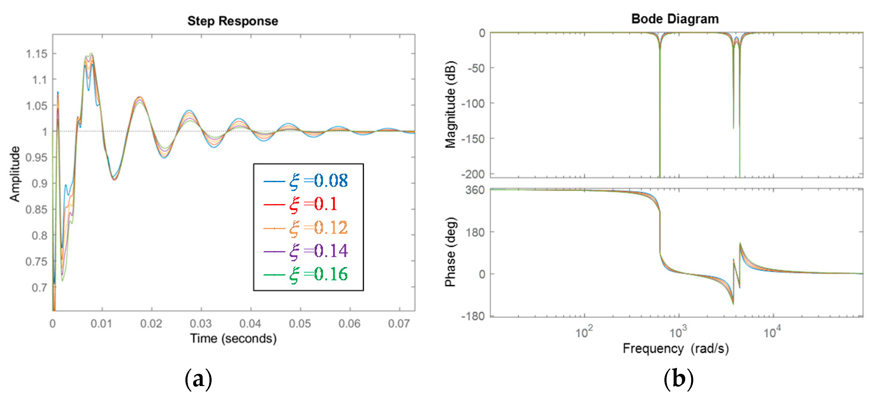
Figure 16.
(a) Graphical representation that shows how sequence decomposition produces the superposition of two currents; a dc current plus a sinusoidal current at 100 Hz, (b) step response of a notch filter tuned at 100 Hz with different damping ratios, (c) response to a sinusoidal input of a notch filter tuned at 100 Hz with different damping ratios, (d) Bode diagrams of a notch filter tuned at 100 Hz with different damping ratios.
Figure 17.
Poles and zeros of the currents for the global closed loop system in the
αβ reference frame for step input references, corresponding to the control of
Figure 14, deduced from the mathematical model of
Table 3, and applied to the numerical scenario of
Appendix B. It is assumed that there is delay in the converter voltage update and the voltage and current filters are not included, i.e.,
Fi(
z) = 1,
Fv(
z)
= 1.
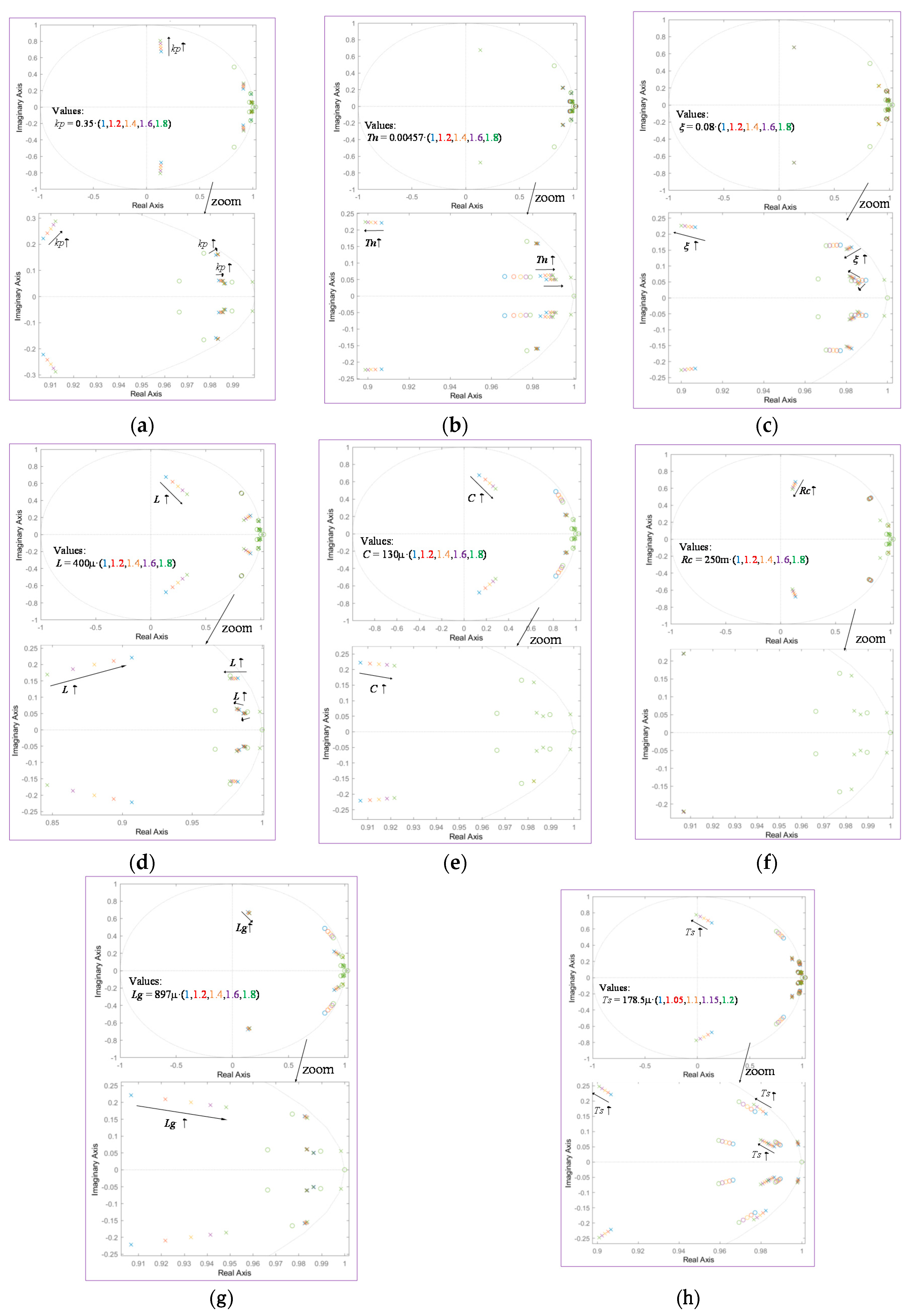
Figure 18.
Variation of the poles and zeros of the output currents of the global closed loop system for step input references, corresponding to the control of
Figure 14, deduced from the mathematical model of
Table 3, and applied to the numerical scenario of
Appendix A. Each parameter is modified as specified. It is assumed that there is delay in the converter voltage update and the voltage and current filters are not included, i.e.,
Fi(
z)
= 1,
Fv(
z)
= 1. (
a)
kp variation; (
b)
Tn variation; (
c)
ξ variation; (
d)
L variation; (
e)
C variation; (
f)
Rc variation; (
g)
Lg variation; (
h)
Ts variation.
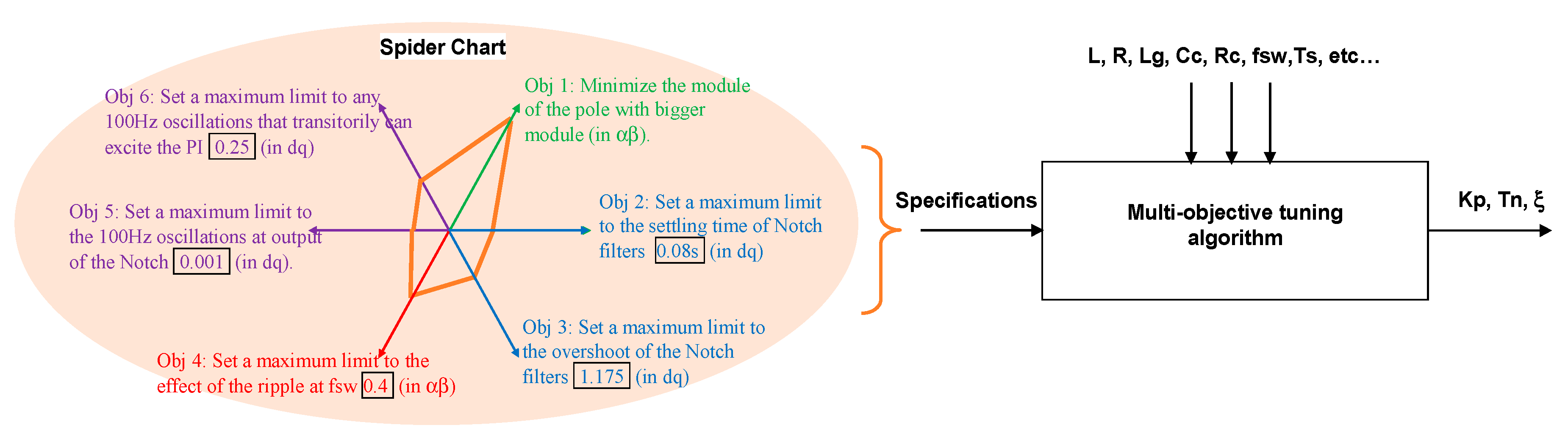
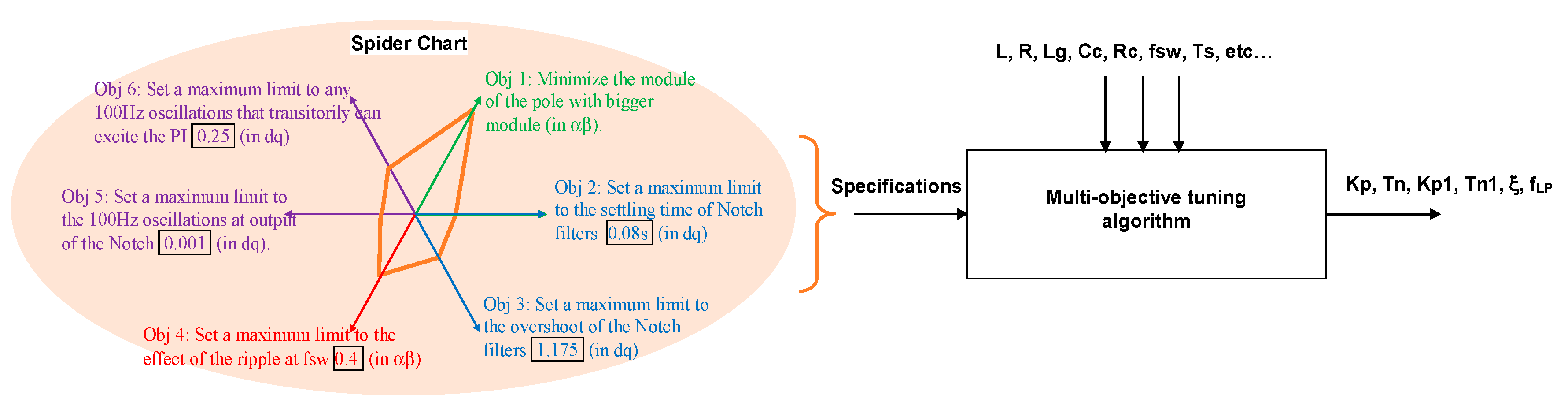
Figure 19.
Multi-objective tuning algorithm based on the optimization of six different objectives.
Figure 19.
Multi-objective tuning algorithm based on the optimization of six different objectives.
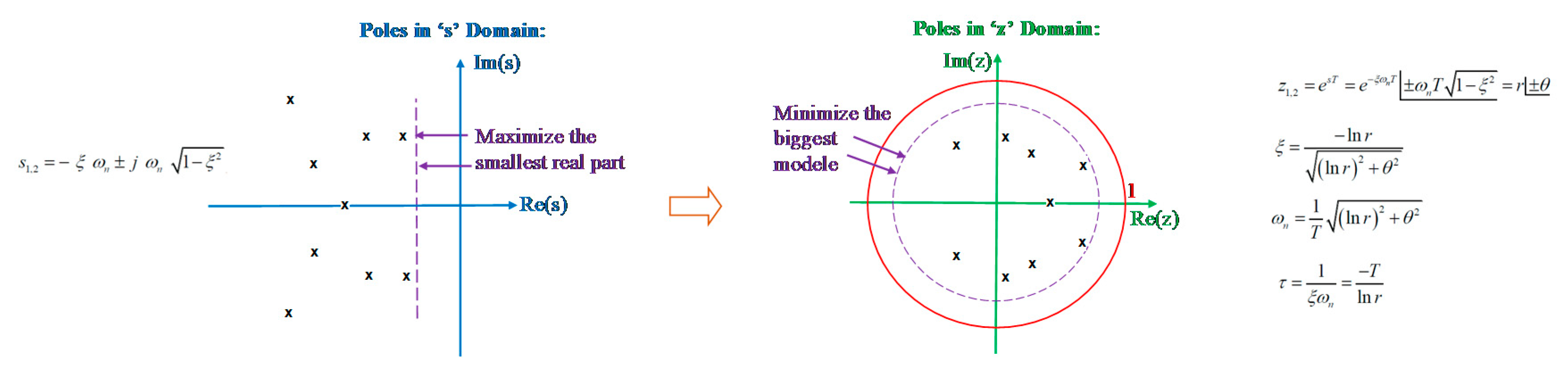
Figure 20.
Module minimization of the pole with the bigger module (dominant pole) in the “z” domain.
Figure 20.
Module minimization of the pole with the bigger module (dominant pole) in the “z” domain.
Figure 21.
Obtained pole-zero map after the search: kp = 0.24, Tn = 0.0065, and ξ = 0.096.
Figure 21.
Obtained pole-zero map after the search: kp = 0.24, Tn = 0.0065, and ξ = 0.096.
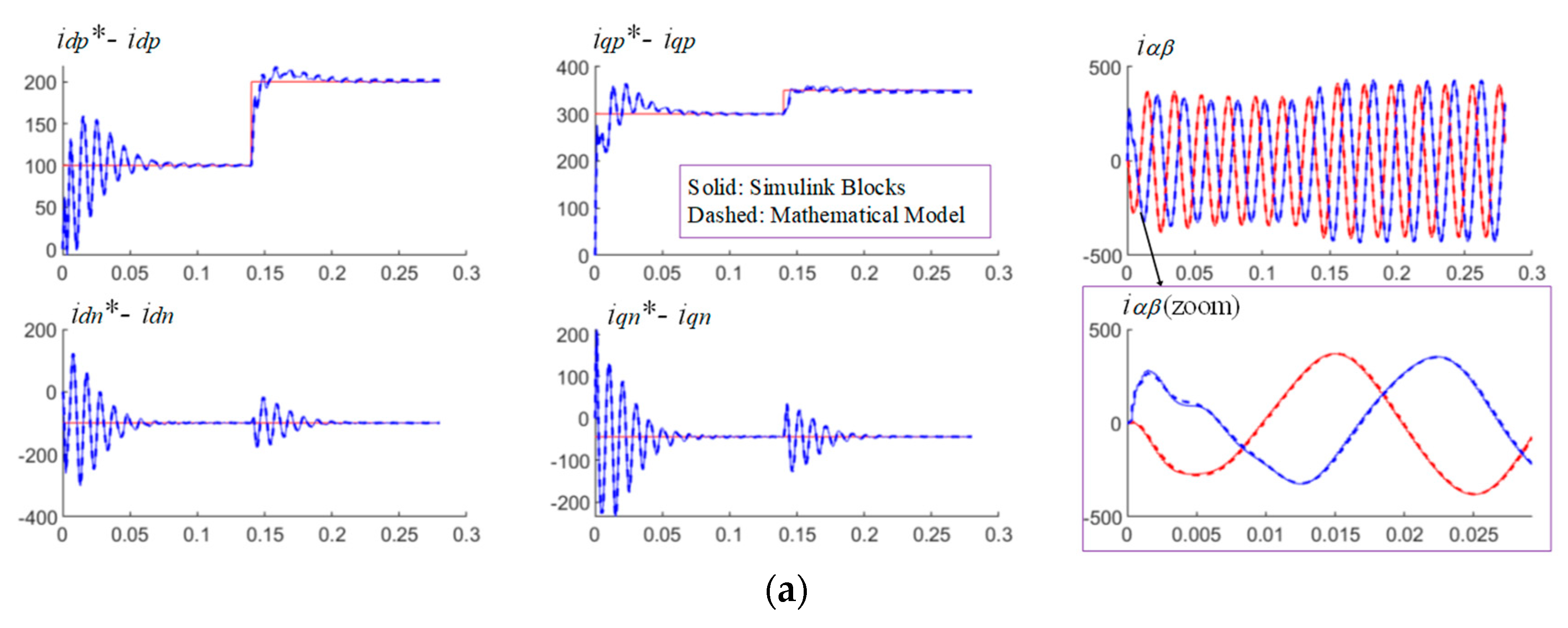
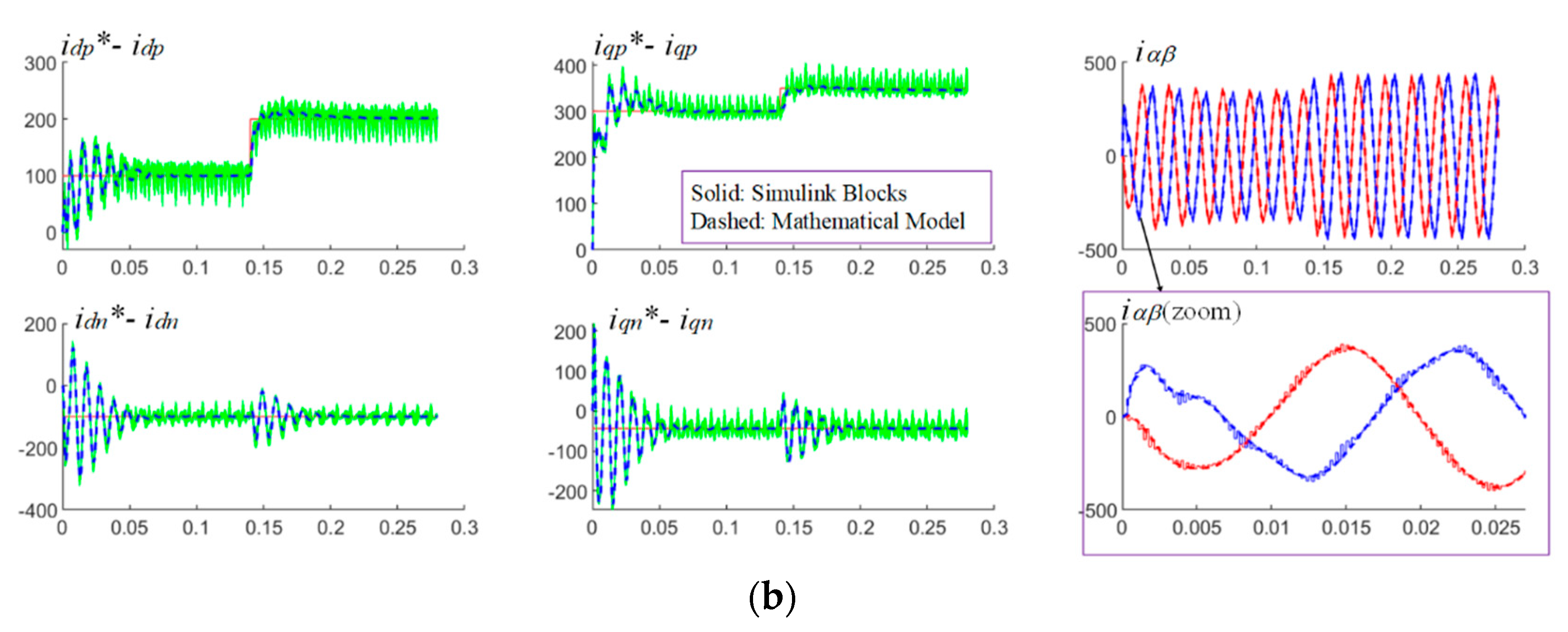
Figure 22.
Superposition of the time-domain responses of the mathematical model proposed in
Table 3 and the control block diagram of
Figure 14 (variables sampled at
Ts) built in Matlab–Simulink blocks. Same input variables are applied at both controls, and the same numerical parameters are used in both models as well (
Appendix B). (
a) Ideal voltage sources are used as an ideal power electronic converter, (
b) A 3L-NPC power electronic converter switched at
fsw is used as an power electronic converter.
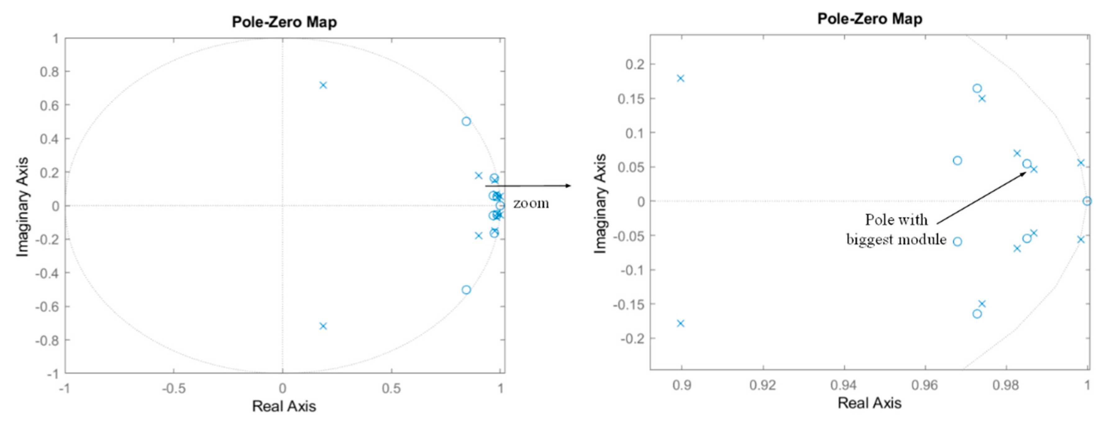
Figure 23.
Obtained pole-zero map after the search: Kp = 0.23, Tn = 0.00487, and ξ = 0.12.
Figure 23.
Obtained pole-zero map after the search: Kp = 0.23, Tn = 0.00487, and ξ = 0.12.
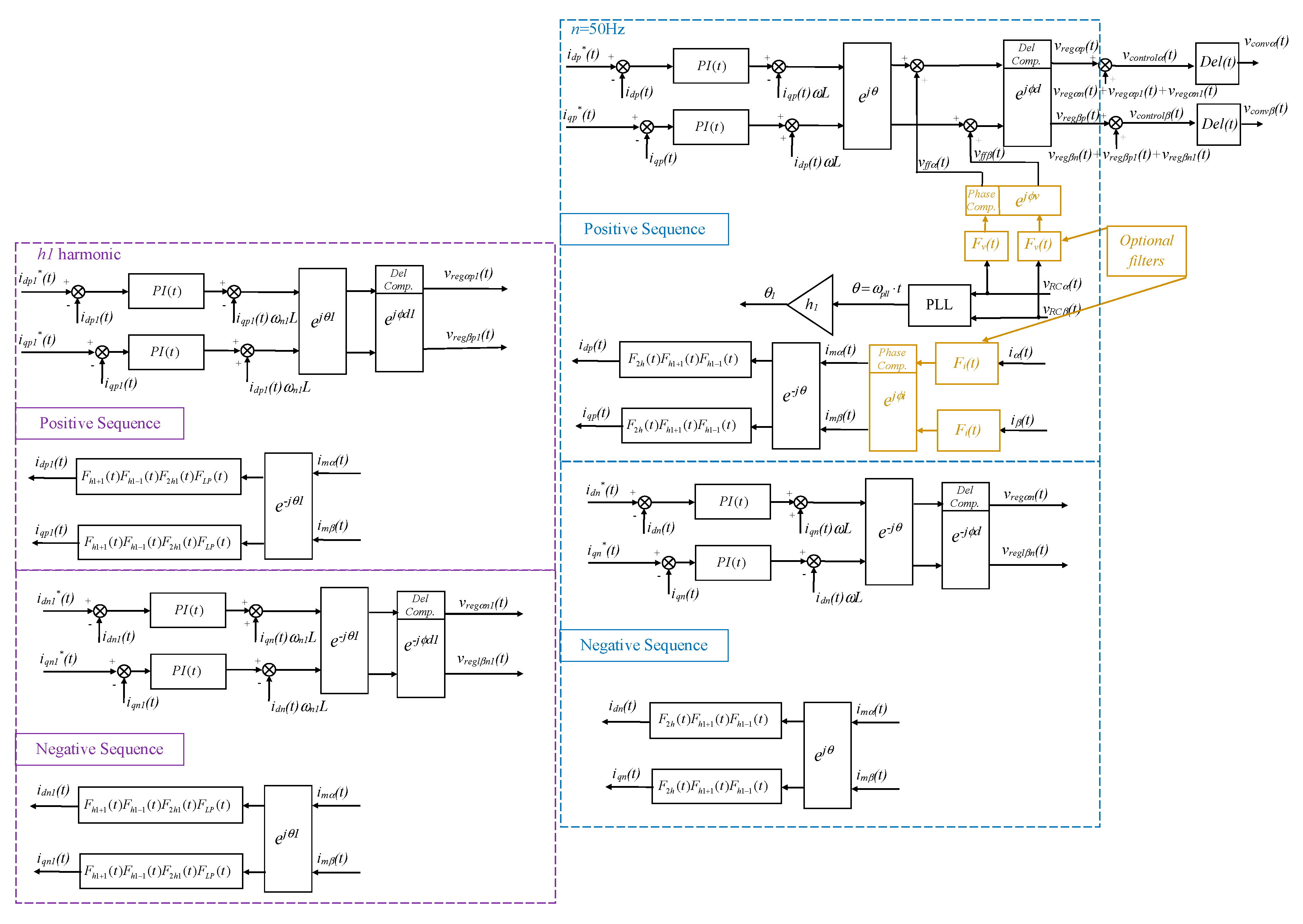
Figure 24.
Fundamental and harmonic current control loops for positive and negative sequences using PI regulators in the dq reference frame: active Filter.
Figure 24.
Fundamental and harmonic current control loops for positive and negative sequences using PI regulators in the dq reference frame: active Filter.
Figure 25.
Bode diagrams derived from the mathematical expressions involved on the ripple transmission from the current measurements to the output converter voltage generated by the control. Numerical values of
Appendix C. (
a) Loop for harmonic
h = 1. (
b) Loop for harmonic
h1 = 13.
Figure 25.
Bode diagrams derived from the mathematical expressions involved on the ripple transmission from the current measurements to the output converter voltage generated by the control. Numerical values of
Appendix C. (
a) Loop for harmonic
h = 1. (
b) Loop for harmonic
h1 = 13.
Figure 26.
Step responses and Bode diagrams of the product of the notch filters; for 50 Hz loops, with different damping ratios. (a) Step responses, (b) Bode diagrams.
Figure 26.
Step responses and Bode diagrams of the product of the notch filters; for 50 Hz loops, with different damping ratios. (a) Step responses, (b) Bode diagrams.
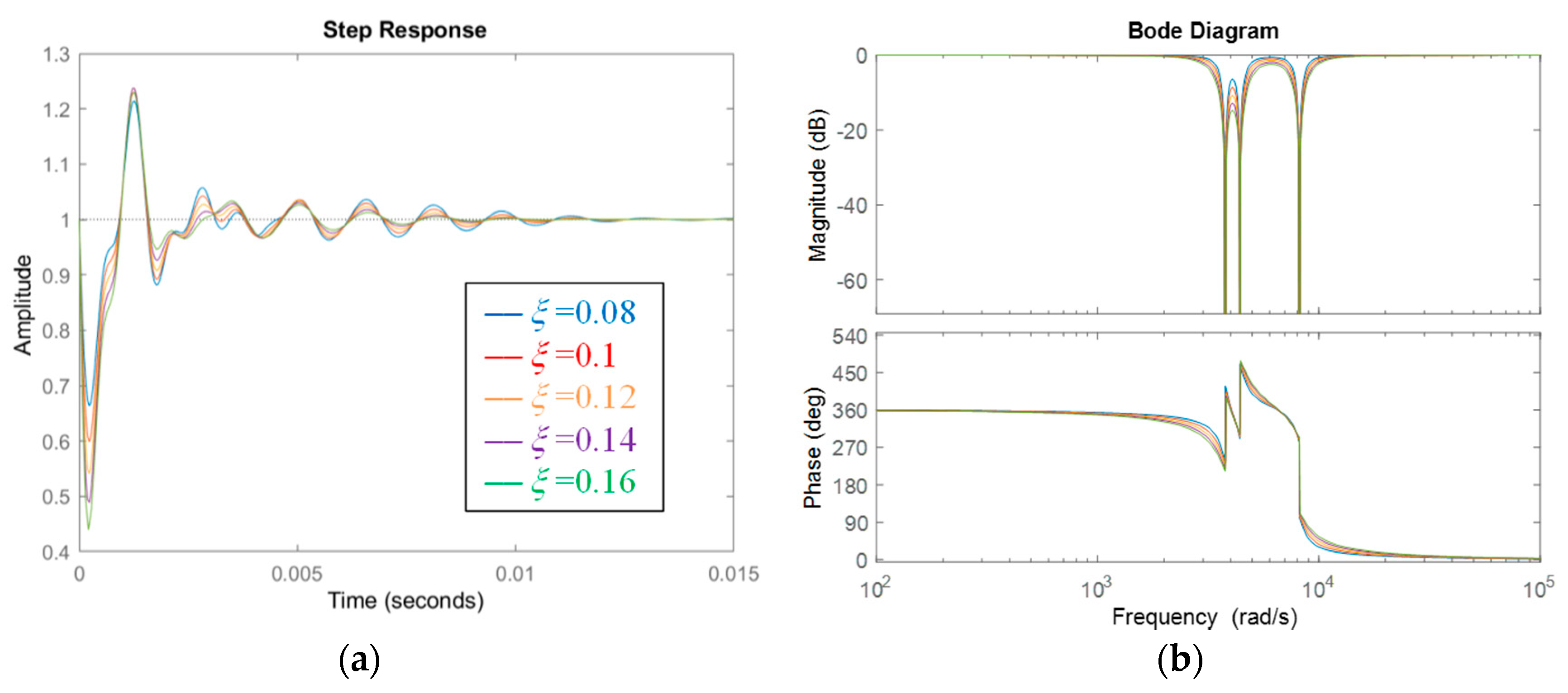
Figure 27.
Step responses and Bode diagrams of product of notch filters: for 650 Hz loops, with different damping ratios. (a) Step responses, (b) Bode diagrams.
Figure 27.
Step responses and Bode diagrams of product of notch filters: for 650 Hz loops, with different damping ratios. (a) Step responses, (b) Bode diagrams.
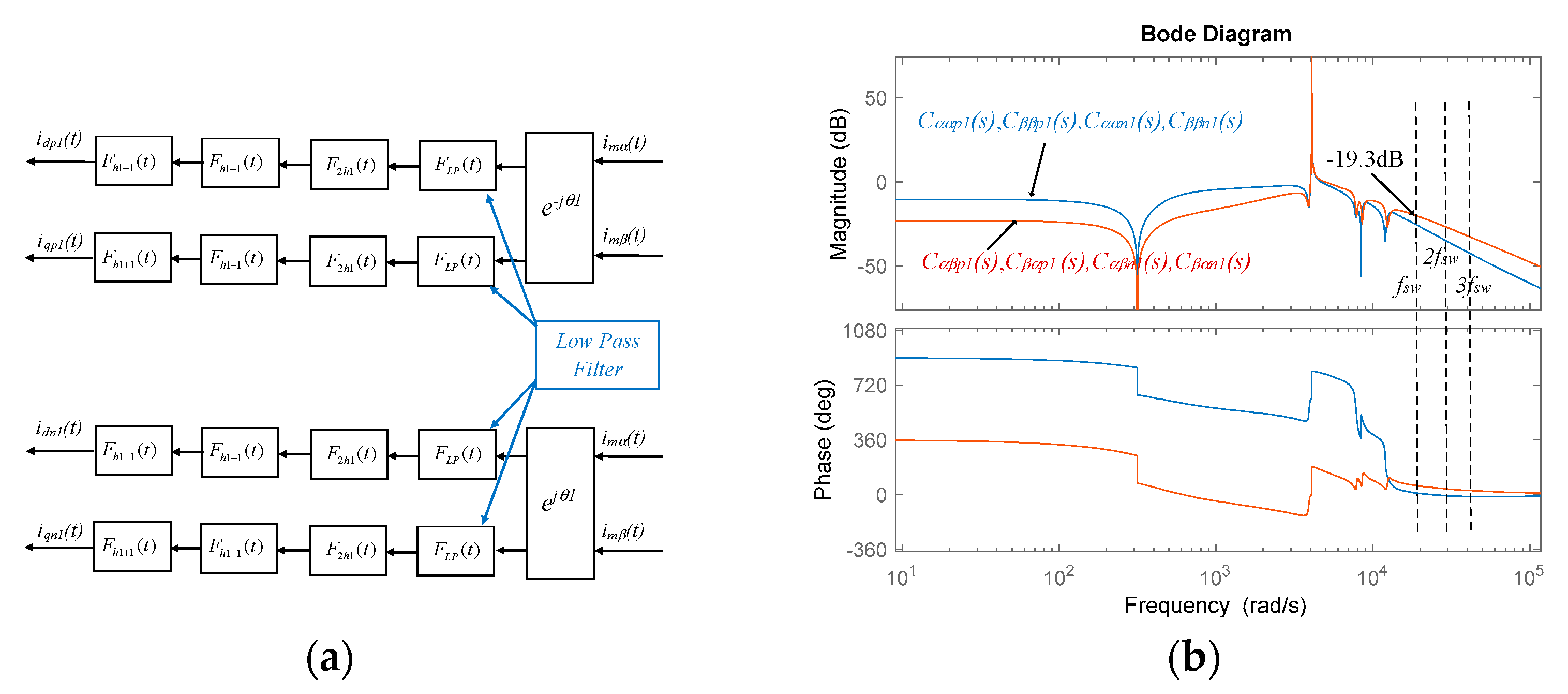
Figure 28.
(
a) Inclusion of the low-pass filter
FLP(
s) at the 650 Hz loops in the dq reference frame (in concordance with block diagram of
Figure 24 and mathematical model of
Table 9 and
Table 10), (
b) Bode diagrams including the low-pass filter at the loop of 650 Hz, which were derived from the mathematical expressions involved on the ripple transmission from the current measurements to the output converter voltage generated by the control. Numerical values of
Appendix C.
Figure 29.
Poles and zeros for the global closed loop system in the
αβ reference frame for step input references, corresponding to the control of
Figure 24, deduced from the mathematical model of
Table 9 and
Table 10, and applied to the numerical scenario of
Appendix C. It is assumed that there is a delay in the converter voltage update and the voltage and current filters are not included, i.e.,
Fi(
z)
= 1,
Fv(
z) = 1. Dependence on parameters has been included as well (there are some poles whose location do not depend on the evaluated parameters).
Figure 30.
Multi-objective tuning algorithm based on the optimization of six different objectives.
Figure 30.
Multi-objective tuning algorithm based on the optimization of six different objectives.
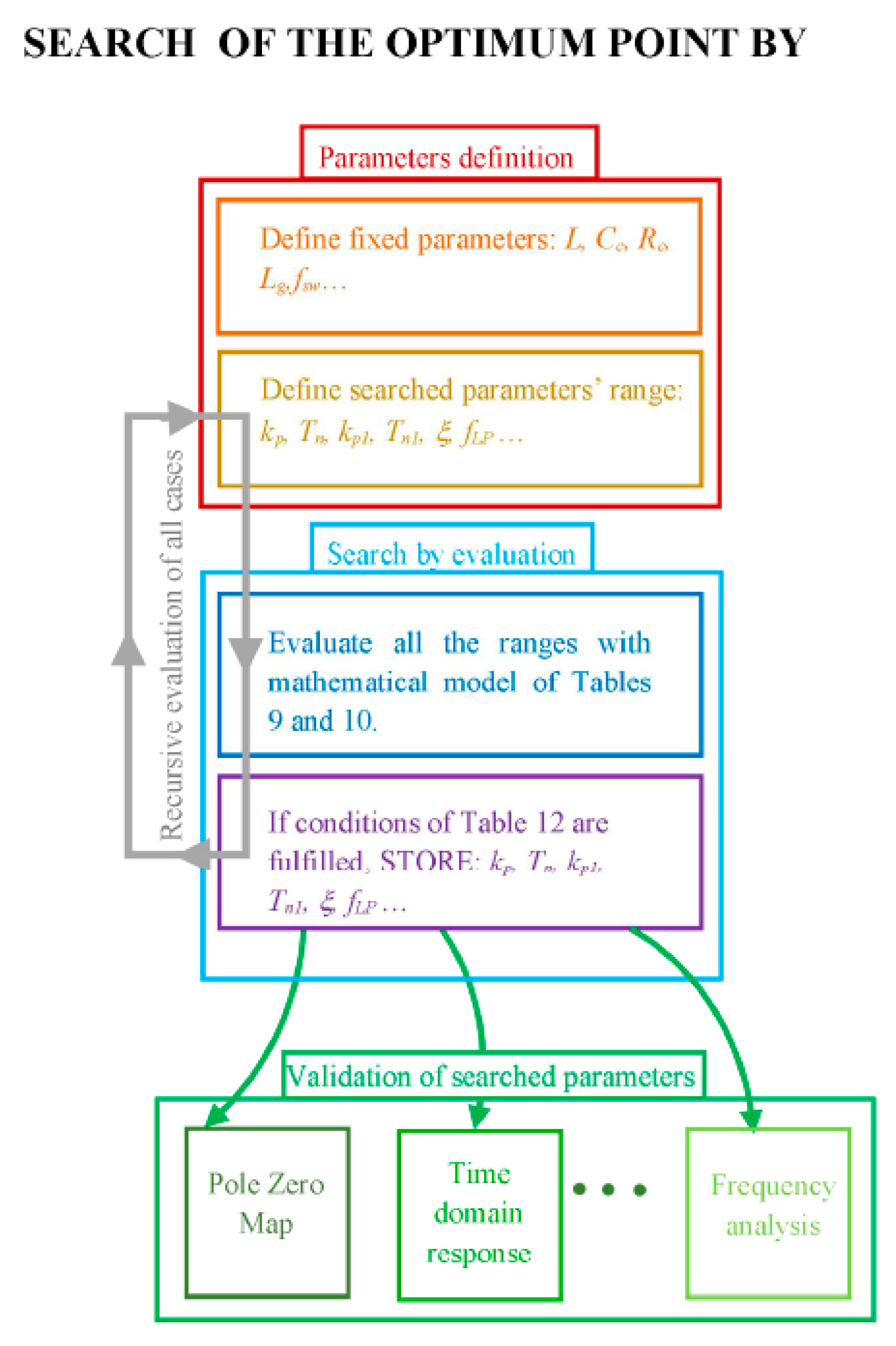
Figure 31.
Conceptual block diagram showing the procedure that can be followed to search the optimum set of parameters for the current control loops. For instance, it can be implemented together with the validation in a unique Matlab program. This procedure can be applied equivalently to the previously studied current controls.
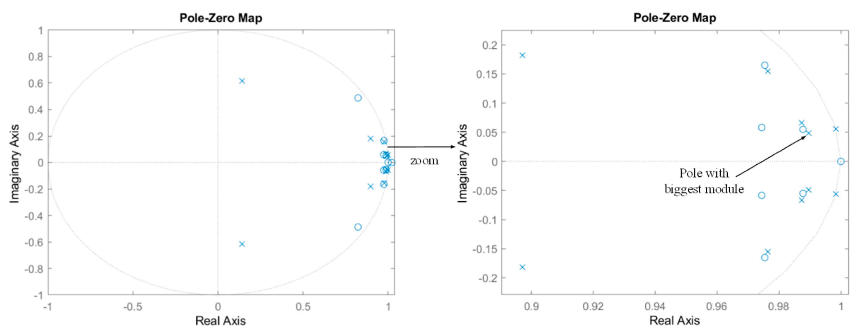
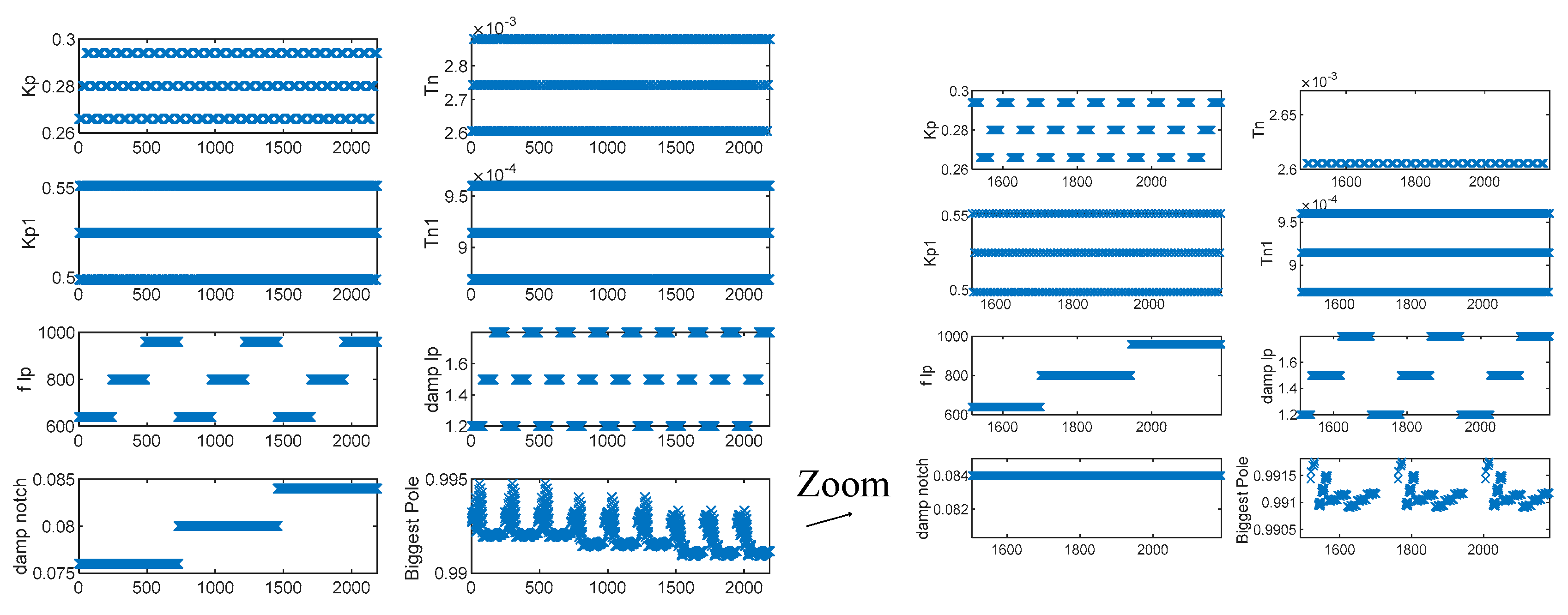
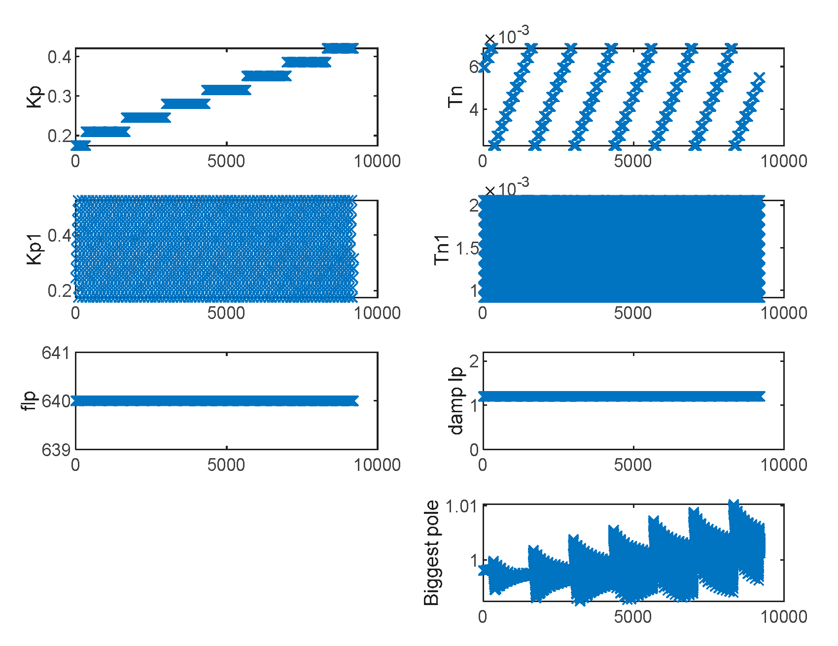
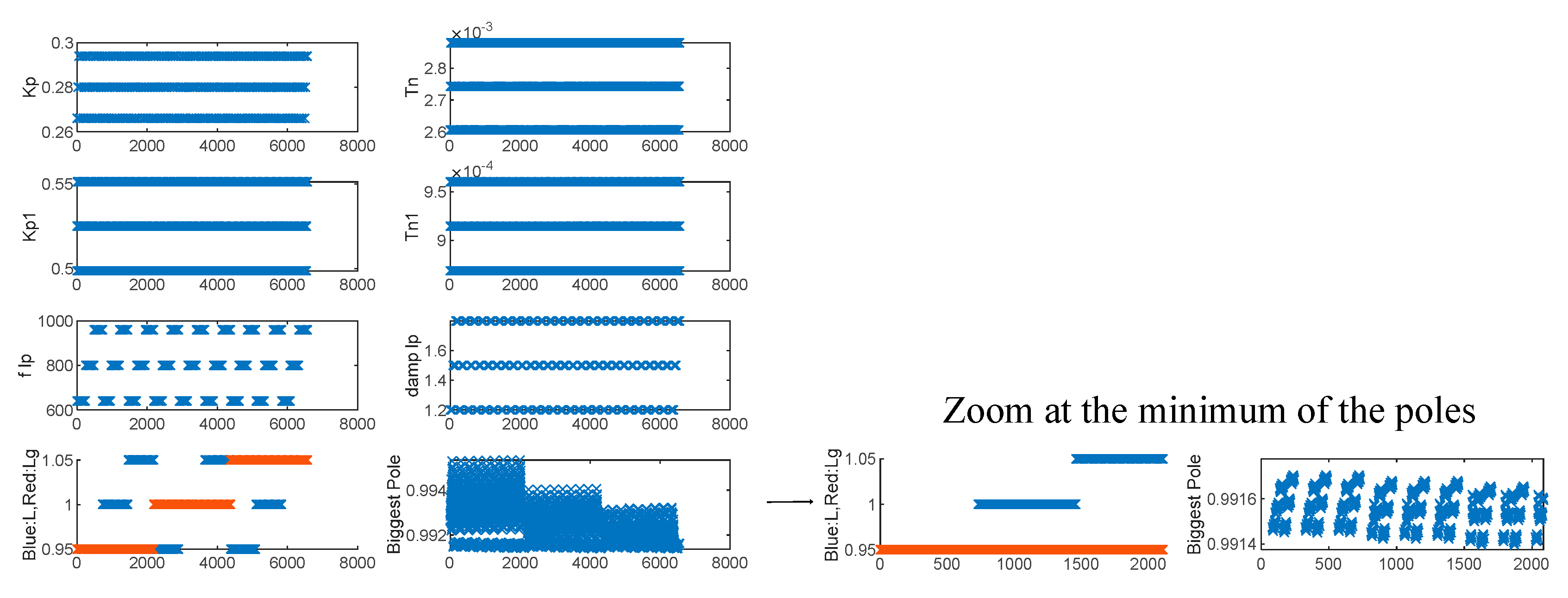
Figure 32.
Parameter variations and poles with the biggest module of each control parameter. From the graph, the control parameters that result from the minimum module pole can be found. Then, other specifications fulfillment should be checked, too.
Figure 32.
Parameter variations and poles with the biggest module of each control parameter. From the graph, the control parameters that result from the minimum module pole can be found. Then, other specifications fulfillment should be checked, too.
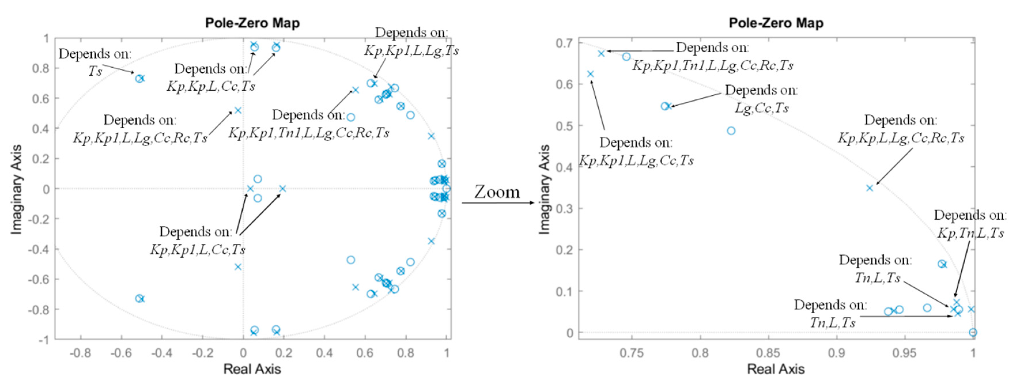
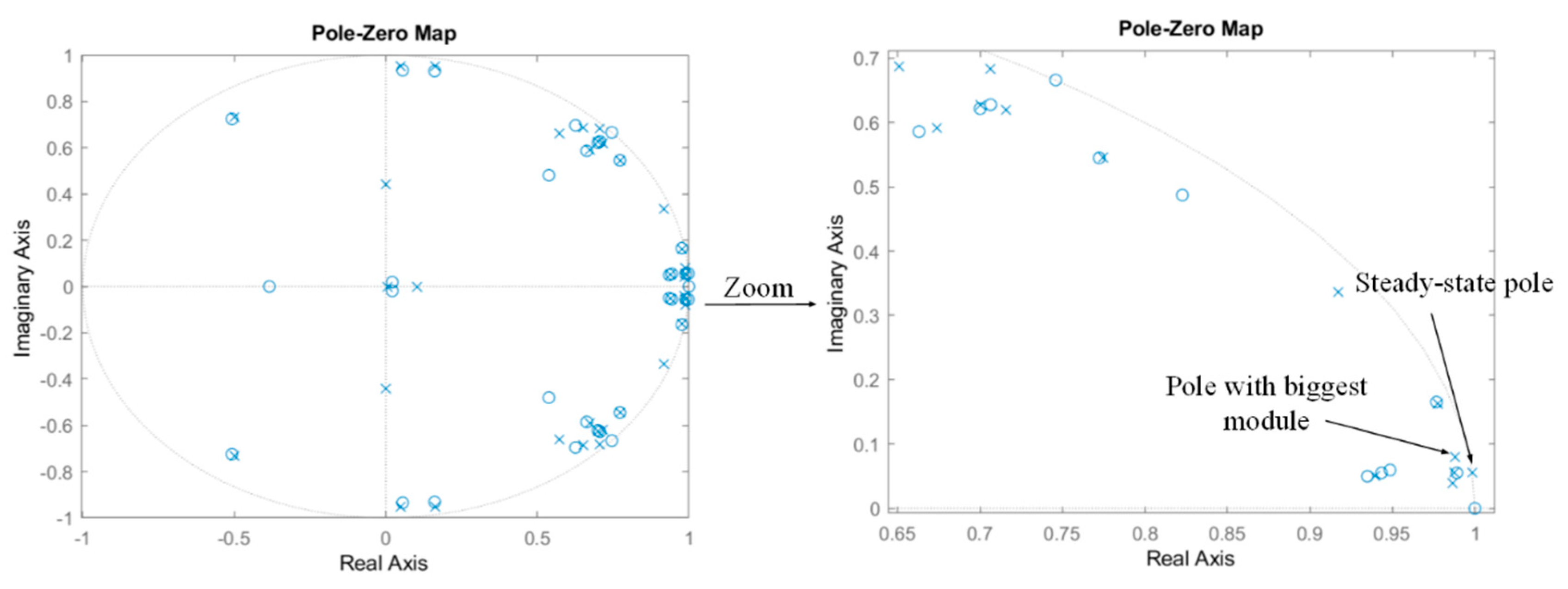
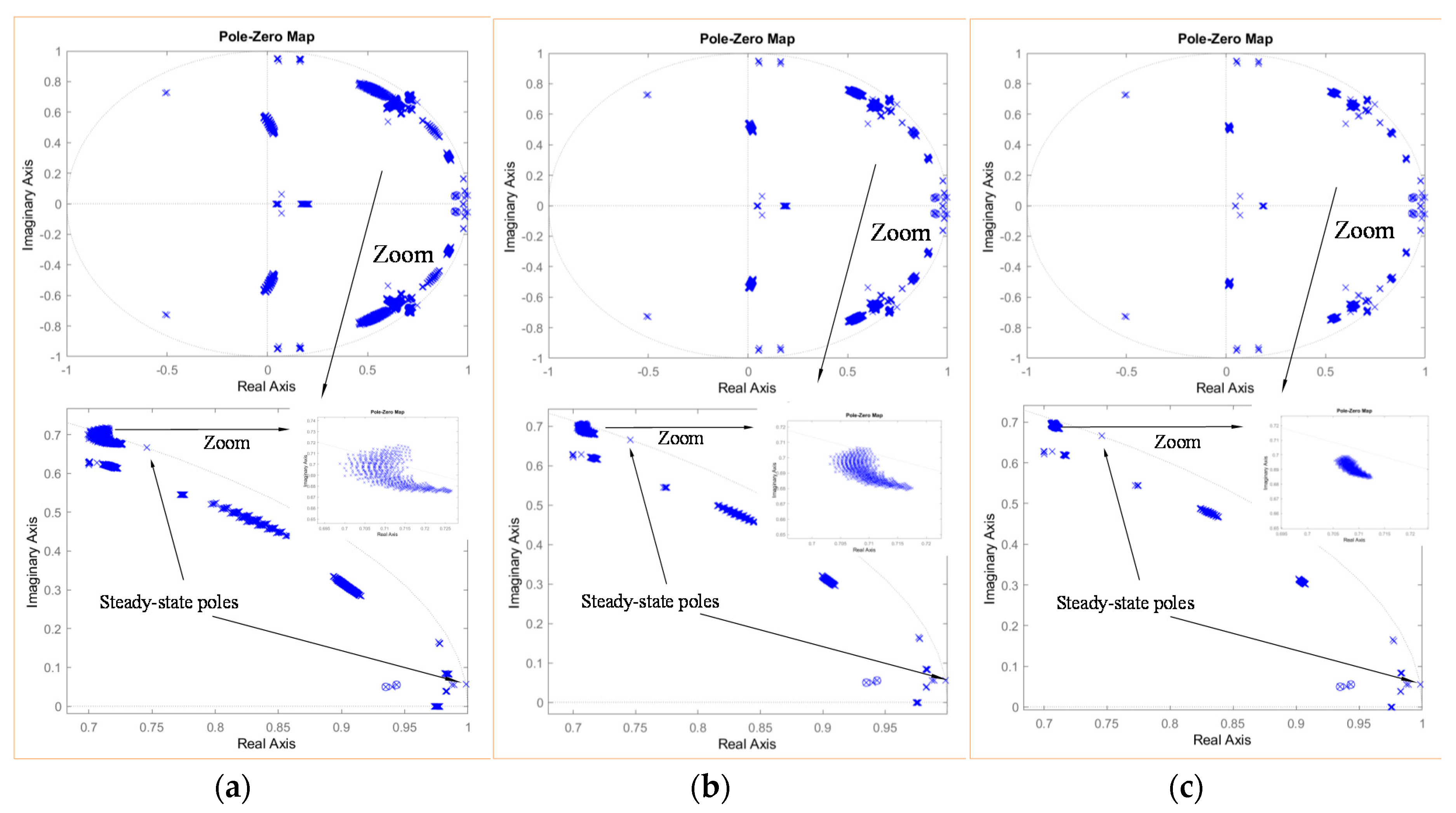
Figure 33.
Pole-zero map (
iα(z)/
idp*(z)) corresponding to the control parameters with a minimum module pole resulting from the previous
Figure 31:
Kp = 0.266,
Tn = 0.0026055,
Kp1 = 0.55125,
Tn1 = 0.00096012,
ξNotch = 0.084,
ξLP = 1.8,
fLP = 960 Hz,
|z|min = 0.9909. It is also checked that this point meets the rest of the specifications of
Table 12 (this information is not included in the graph for simplicity).
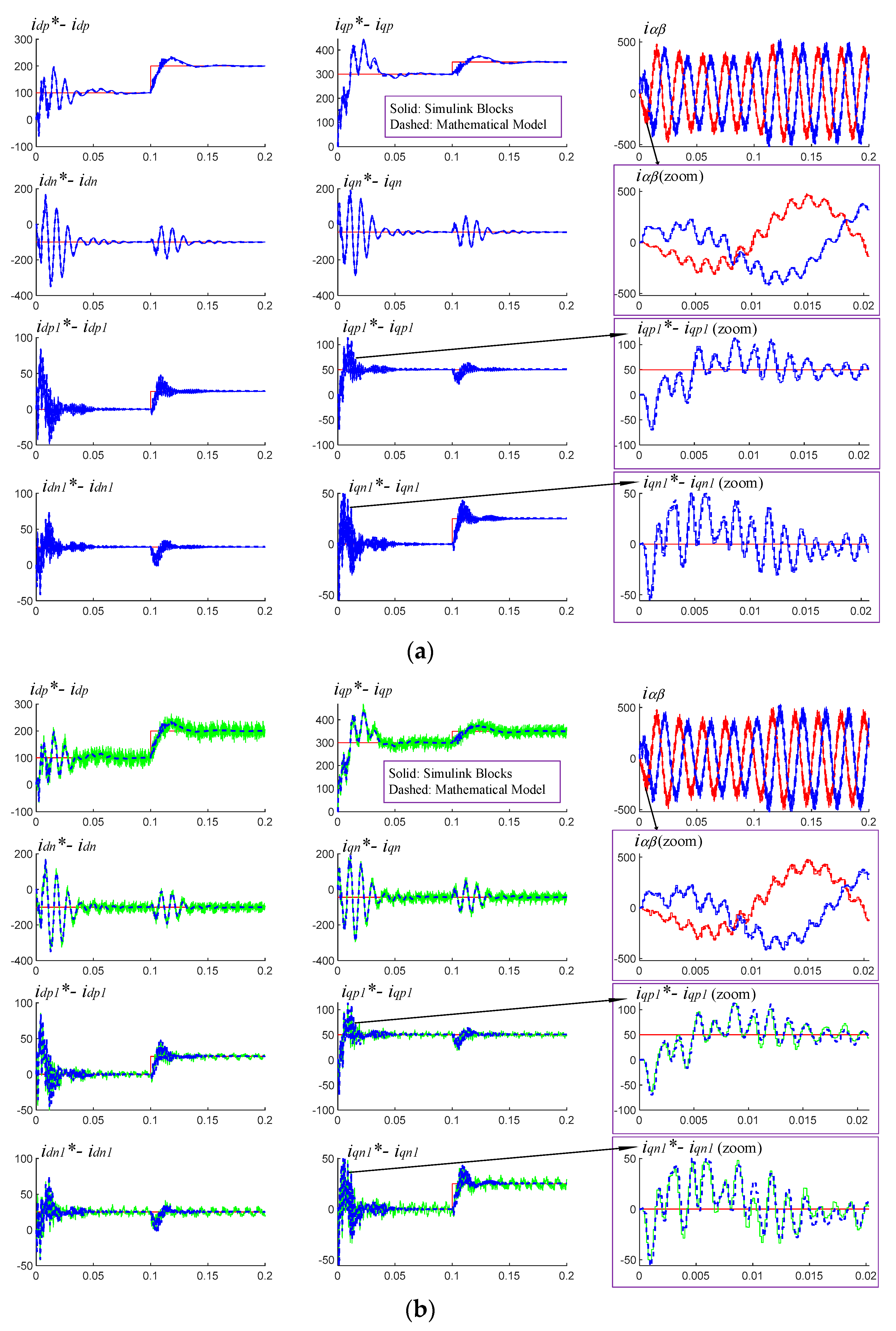
Figure 34.
Superposition of the time-domain responses of the mathematical model proposed in
Table 9 and
Table 10 and the control block diagram of
Figure 24 (variables sampled at
Ts), built in Matlab–Simulink blocks. The same input variables are applied at both controls, and the same numerical parameters are used in both models as well (
Appendix C). (
a) Ideal voltage sources are used as an ideal power electronic converter, (
b) a 3L-NPC power electronic converter switched at
fsw is used as power electronic converter.
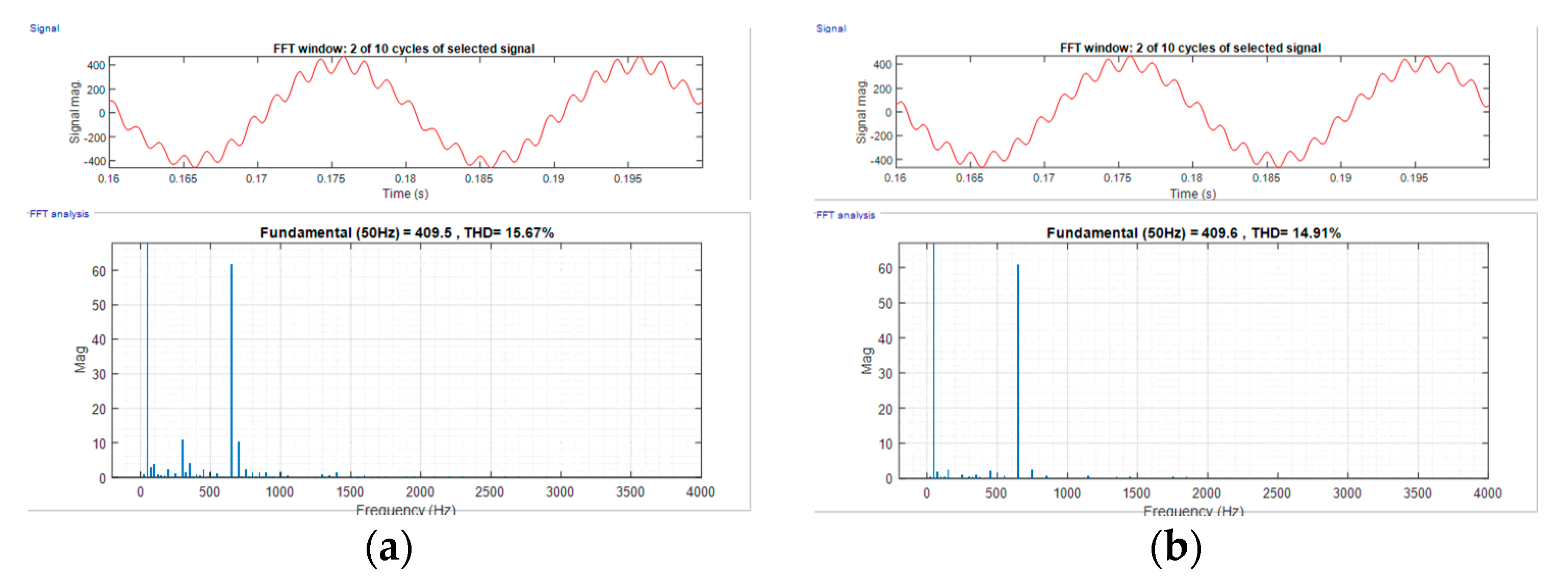
Figure 35.
Spectrum of the currents exchanged with the grid at different fsw. (a) ig at fsw = 1/5800 Hz, (b) ig at fsw = 1/6500 Hz.
Figure 35.
Spectrum of the currents exchanged with the grid at different fsw. (a) ig at fsw = 1/5800 Hz, (b) ig at fsw = 1/6500 Hz.
Figure 36.
Parameter variations and poles with the biggest module of each control parameter. In this case, a stable and unstable set of control parameters is found.
Figure 36.
Parameter variations and poles with the biggest module of each control parameter. In this case, a stable and unstable set of control parameters is found.
Figure 37.
Parameter variations and search of the poles with a maximum module. Evaluation of the poles when parameters Lg and L are varied in a range of ±5% from its actual value (uncertainty of ±5%).
Figure 37.
Parameter variations and search of the poles with a maximum module. Evaluation of the poles when parameters Lg and L are varied in a range of ±5% from its actual value (uncertainty of ±5%).
Figure 38.
Robustness under uncertainty of all electric parameters. The control parameters are set constant (Kp = 0.266, Tn = 0.0026055, Kp1 = 0.55125, Tn1 = 0.00096012, ξNotch = 0.084, ξLP = 1.8, fLP = 960 Hz, |z|min = 0.9909) and all the electric parameters; L, Cc, Lg, Rc, R, and Rg are varied; (a) ±10% range (steps 5%), (b) ±5% range (steps 2.5%), (c) ±2.5% range (steps 1.25%).
Table 1.
Mathematical model of the control of
Figure 2. It can be directly implemented sequentially in a Matlab program.
c2d: continuous to discrete. The discretization method used in this paper is ZOH.
Table 1.
Mathematical model of the control of
Figure 2. It can be directly implemented sequentially in a Matlab program.
c2d: continuous to discrete. The discretization method used in this paper is ZOH.
Measurements (filter & phase shift compensation at fundamental frequency):
| |
Control parts:
| | |
| |
| |
| |
| |
| | | |
| | | |
Control: Regulators side:
| Control: Regulator side + Feed forward term:
|
Converter’s delay and compensation:
| |
| | | |
| | | |
Filter and Grid:
|
|
Connection of all the elements: Derivation of the ‘Global model matrix’, through the ‘Connect’ function from Matlab (the choice of the output variables is not unique):
|
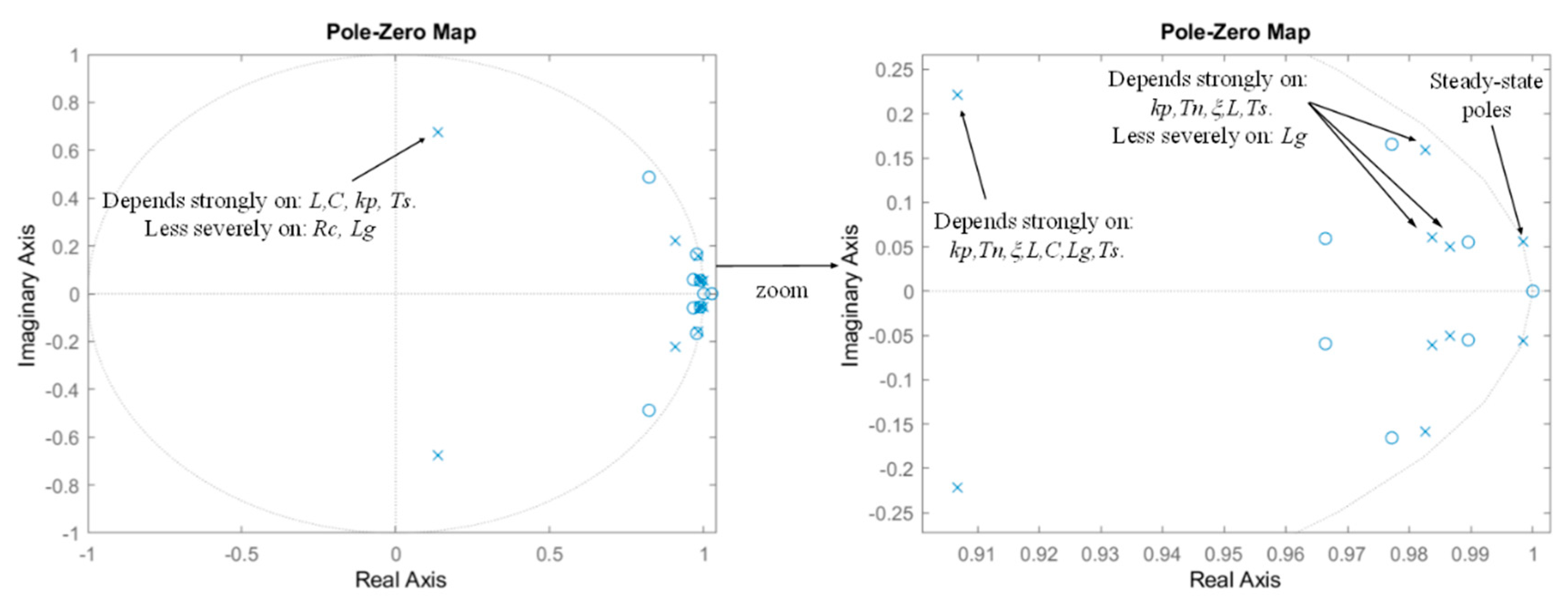
Table 2.
Characteristics of each pole for this specific numerical example.
Table 2.
Characteristics of each pole for this specific numerical example.
| Poles | Characteristics | Sensitivity to Parameters |
|---|
1.090766718154714 × 10⁻¹ + 5.701504905811328 × 10⁻¹i
1.090766718154714 × 10⁻¹ − 5.701504905811328 × 10⁻¹i | |z| = 0.58049,
ωn = 8.32 rd/s, ξn = 0.366 | Depends strongly on: L, C, Rc, kp, Ts.
Less severely on: Lg |
1.894264790299348 × 10⁻¹ + 5.840850254455814 × 10⁻¹i
1.894264790299348 × 10⁻¹ − 5.840850254455814 × 10⁻¹i | |z| = 0.61403,
ωn = 0.755 rd/s, ξn = 0.362 | Depends strongly on: L, C, Rc, kp, Ts.
Less severely on: Lg |
8.529727735128836 × 10⁻¹ + 1.431145783233994 × 10⁻¹i
8.529727735128836 × 10⁻¹ − 1.431145783233994 × 10⁻¹i | |z| = 0.86489,
ωn = 1240 rd/s, ξn = 0.658 | Depends strongly on: kp, Tn, L, C, Lg, Ts. |
9.472162630104273 × 10⁻¹ + 3.787043727243775 × 10⁻²i
9.472162630104273 × 10⁻¹ − 3.787043727243775 × 10⁻²i | |z| = 0. 9479,
ωn = 374 rd/s, ξn = 0.8 | Depends strongly on: kp, Tn, L, Ts.
Less severely on: Lg |
9.614484330375144 × 10⁻¹ + 1.473576487639808 × 10⁻¹i
9.614484330375144 × 10⁻¹ − 1.473576487639808 × 10⁻¹i | |z|= 0.9726,
ωn = 866 rd/s, ξn = 0.179 | Depends strongly on: kp, Tn, L, Lg, Ts. |
9.984280729837364 × 10⁻¹ + 5.604804257701512 × 10⁻²i
9.984280729837364 × 10⁻¹ − 5.604804257701512 × 10⁻²i | |z| = 1,
ωn = 314.16 rd/s, ξn = 0 | Steady-state poles |
Table 3.
Mathematical model of the studied control. Control equations for loops dedicated to harmonics h = 1 (50 Hz) that can be implemented sequentially in a Matlab program for instance. c2d: continuous to discrete. The method used in this paper is ZOH.
Table 3.
Mathematical model of the studied control. Control equations for loops dedicated to harmonics h = 1 (50 Hz) that can be implemented sequentially in a Matlab program for instance. c2d: continuous to discrete. The method used in this paper is ZOH.
| | |
| | |
| |
| |
| |
| |
| | | |
| | | |
|
| |
| |
| |
| |
| | | |
| | | |
| |
|
Connection of all the elements including the grid, filter and converter models (Table 1): Derivation of the ‘Global model matrix’, through the ‘Connect’ function from Matlab (the choice of the output variables is not unique):
|
Table 4.
Objectives of the notch filter and the required damping values.
Table 4.
Objectives of the notch filter and the required damping values.
| Objective | Damping Necessity |
|---|
| Minimize oscillations of 100 Hz at steady state | ξ ↑ |
| Minimize the transient response (damping time) to the step input | ξ ↑ |
| Minimize the transient response (damping time) to the sinusoidal input | ξ ↑ |
| Minimize the overshoot (peak value) to the step input | ξ ↓ |
| Minimize the overshoot (peak value) to the sinusoidal input | ξ ↑ |
Table 5.
Characteristics of each pole for this specific numerical example.
Table 5.
Characteristics of each pole for this specific numerical example.
| Poles | Characteristics | Sensitivity to Parameters |
|---|
1.364670911241526 × 10⁻¹ + 6.756530921004849 × 10⁻¹i
1.364670911241526 × 10⁻¹ − 6.756530921004849 × 10⁻¹i | |z| = 0.6893,
ωn = 7960 rd/s, ξn = 0.262 | Depends strongly on: L, C, kp, Ts.
Less severely on: Rc, Lg |
9.067319297256008 × 10⁻¹ + 2.215731584333249 × 10⁻¹i
9.067319297256008 × 10⁻¹ − 2.215731584333249 × 10⁻¹i | |z| = 0.93341,
ωn = 1400 rd/s, ξn = 0.276 | Depends strongly on: kp, Tn, ξ, L, C, Lg, Ts |
9.837247566747704 × 10⁻¹ + 6.095823423310127 × 10⁻²i
9.837247566747704 × 10⁻¹ − 6.095823423310127 × 10⁻²i | |z| = 0.98561,
ωn = 356 rd/s, ξn = 0.228 | Depends strongly on: kp, Tn, ξ, L, Ts.
Less severely on: Lg |
9.865149131707045 × 10⁻¹ + 5.022937190387527 × 10⁻²i
9.865149131707045 × 10⁻¹ − 5.022937190387527 × 10⁻²i | |z| = 0.9877,
ωn = 293 rd/s, ξn = 0.235 | Depends strongly on: kp, Tn, ξ, L, Ts.
Less severely on: Lg |
9.825111447917705 × 10⁻¹ + 1.587919854687506 × 10⁻¹i
9.825111447917705 × 10⁻¹ − 1.587919854687506 × 10⁻¹i | |z| = 0.99526,
ωn = 898 rd/s, ξn = 0.0296 | Depends strongly on: kp, Tn, ξ, L, Ts.
Less severely on: Lg |
9.984280729580852 × 10⁻¹ + 5.604804256738856 × 10⁻²i
9.984280729580852 × 10⁻¹ − 5.604804256738856 × 10⁻²i | |z| = 1,
ωn = 314.16 rd/s, ξn = 0 | Steady-state poles |
Table 6.
Multi-objective optimization table.
Table 6.
Multi-objective optimization table.
| Objective | Mathematical Expression | Possible Value for Specification | Example of Code Program (see Matlab Help for More Information of the Functions Shown) |
|---|
| Minimize the module of the pole with a bigger module, excluding the steady-state poles (in the αβ reference frame) | Module of poles of: | Find the minimum | [poles,zeros] = pzmap(Gmm);
Mod_pol_max = max(abs(poles)); |
| Set a maximum limit to the settling time of notch filters to the step input (in the dq reference frame) | | <0.08 | F = (s^2 + w^2)/(s^2 + 2 × damp×w×s + w^2);
F_inf = stepinfo(F);
F_inf.SettlingTime |
| Set a maximum limit to the overshoot of the notch filters to the step input (in the dq reference frame) | | <1.175 | F = (s^2 + w^2)/(s^2 + 2 × damp × w × s + w^2); F_inf = stepinfo(F);
F_inf.Peak |
| Set a maximum limit to the effect of the ripple at fsw in the control loops (in the αβ reference frame) | Cααp, Cαβp, Cβαp, Cββp and Cααn, Cαβn, Cβαn, Cββn | <0.4 | [Magsw1,phase,wout]= bode(Cal_al_p, wsw); [Magsw2,phase,wout]= bode(Cbe_al_p, wsw); |
| Set a maximum limit to the 100 Hz oscillations at output of the notch (in the dq reference frame) | | <0.001 | F = (s^2 + w^2)/(s^2 + 2 × damp × w × s + w^2); [Mag100_F,phase,wout] = bode(F, 100 × 2 × pi); |
| Set a maximum limit to any 100 Hz oscillations that transitorily can excite the PI (in the dq reference frame) | | <0.25 | PI = (Kp + (Kp/Tn)/(s));
[Mag100_PI,phase,wout] = bode(PI, 100 × 2 × pi) |
Table 7.
Obtained values after the multi-objective search: kp = 0.24, Tn = 0.0065, and ξ = 0.096.
Table 7.
Obtained values after the multi-objective search: kp = 0.24, Tn = 0.0065, and ξ = 0.096.
| Objective | Value for Specification | Obtained Results |
|---|
| Minimize the module of the pole with the bigger module, excluding the steady-state poles (in the αβ reference frame) | <1 | |z| = 0.99086, ωn = 281 rd/s, ξn = 0.183
0.9896613162011 + 4.886042548262 × 10⁻²i
0.9896613162011 − 4.886042548262 × 10⁻²i |
| Set a maximum limit to the effect of the ripple at fsw in the control loops (in the αβ reference frame) | <0.4 | Cααp(ωsw) = Cββp(ωsw) = Cααn(ωsw) = Cββn(ωsw)= 0.239 (−12.4 dB)
Cαβp(ωsw) = Cβαp(ωsw) = Cαβn(ωsw) = Cβαn(ωsw)= 0.125 (−18 dB) |
| Set a maximum limit to the settling time of notch filters to the step input (in the dq reference frame) | <0.08 | 0.06378 |
| Set a maximum limit to the overshoot of the notch filters to the step input (in the dq reference frame) | <1.25 | 1.1226 |
| Set a maximum limit to the 100 Hz oscillations at the output of the notch (in the dq reference frame) | <0.0001 | 7.07 × 10⁻⁸ (−143 dB) |
| Set a maximum limit to any 100 Hz oscillations that transitorily can excite the PI (in the dq reference frame) | <0.25 | 0.2483 (−12.1 dB) |
Table 8.
Obtained values after the multi-objective search with Rc = 50 × 10−3 Ω: kp = 0.23, Tn = 0.00487, and ξ = 0.12.
Table 8.
Obtained values after the multi-objective search with Rc = 50 × 10−3 Ω: kp = 0.23, Tn = 0.00487, and ξ = 0.12.
| Objective | Value for Specification | Obtained Results |
|---|
| Minimize the module of the pole with bigger module, excluding the steady-state poles (in the αβ reference frame) | <1 | |z| = 0.9878, ωn = 273 rd/s, ξn = 0.25
0.9867775356891335 + 4.661389975464711 × 10⁻²i
0.9867775356891335 − 4.661389975464711 × 10⁻²i |
| Minimize the effect of the ripple at fsw in the control loops (in the αβ reference frame) | <0.25 | Cααp(ωsw) = Cββp(ωsw) = Cααn(ωsw) = Cββn(ωsw)= 0.2317 (−12.7 dB)
Cαβp(ωsw) = Cβαp(ωsw) = Cαβn(ωsw) = Cβαn(ωsw)= 0.125 (−18 dB) |
| Minimize the settling time of notch filters to the step input (in the dq reference frame) | <0.08 | 0.0534 |
| Minimize the overshoot of the notch filters to the step input (in the dq reference frame) | <1.175 | 1.137 |
| Minimize 100 Hz oscillations at output of the notch (in the dq reference frame) | <0.0001 | 3.98 × 10⁻¹⁵ (−288 dB) |
| Minimize any 100 Hz oscillations that transitorily can excite the PI (in the dq reference frame) | <0.25 | 0.2317 (−12.7 dB) |
Table 9.
Mathematical model of the studied control. Control equations for loops dedicated to harmonic
h1 = 1 (50 Hz) that can be implemented sequentially in a Matlab program (requires
Table 10 to be completed).
Table 9.
Mathematical model of the studied control. Control equations for loops dedicated to harmonic
h1 = 1 (50 Hz) that can be implemented sequentially in a Matlab program (requires
Table 10 to be completed).
| | |
| | |
| | |
| | |
| |
| |
| |
| |
| | | |
| | | |
|
| |
| |
| |
| |
| | | |
| | | |
|
Table 10.
Mathematical model of the studied. Control equations for loops dedicated to harmonic
h = 13 (650 Hz) that can be implemented sequentially in a Matlab program (requires
Table 9 to be completed).
Table 10.
Mathematical model of the studied. Control equations for loops dedicated to harmonic
h = 13 (650 Hz) that can be implemented sequentially in a Matlab program (requires
Table 9 to be completed).
| | |
| | |
| | |
| | |
| | |
| | |
| |
| |
| |
| |
| | | |
| | | |
| |
| |
| |
| |
| |
| | | |
| | | |
|
|
Connection of all the elements including the grid, filter and converter models (Table 1): Derivation of the ‘Global model matrix’, through the ‘Connect’ function from Matlab (the choice of the output variables is not unique):
|
Table 11.
Harmonics that are present in each loop of the control and therefore need to be filtered with notch filters: h = 1 (50 Hz), h1 = 13 (650 Hz). Colors are used to easy follow correspondence.
Table 11.
Harmonics that are present in each loop of the control and therefore need to be filtered with notch filters: h = 1 (50 Hz), h1 = 13 (650 Hz). Colors are used to easy follow correspondence.
| Current References | Values | Actual Currents | Components |
|---|
| DC (h-h) | 100 Hz (h + h) | 600 Hz (h1-h) | 700 Hz (h1 + h) | 1300 Hz (h1 + h1) |
|---|
| idp* | 100 A | idp | 100 A | 230 A | 90 A | 29 A | 0 |
| iqp* | 200 A | iqp | 200 A | 230 A | 90 A | 29 A | 0 |
| |ip| | 224 A | | | | | | |
| idn* | 150 A | idn | 150 A | 224 A | 29 A | 90 A | 0 |
| iqn* | −175 A | iqn | 175 A | 224 A | 29 A | 90 A | 0 |
| |in| | 230 A | | | | | | |
| idp1* | −50 A | idp1 | 50 A | 0 | 224 A | 230 A | 29 A |
| iqp1* | 75 A | iqp1 | 75 A | 0 | 224 A | 230 A | 29 A |
| |ip1| | 90A | | | | | | |
| idn1* | 25 A | idn1 | 25 A | 0 | 230 A | 224 A | 90 A |
| iqn1* | −15 A | iqn1 | 15 A | 0 | 230 A | 224 A | 90 A |
| |in1| | 29 A | | | | | | |
Table 12.
Multi-objective optimization table.
Table 12.
Multi-objective optimization table.
| Objective | Mathematical Expression | Possible Value for Specification | Example of Code Program
(See Matlab Help for More Information of the Functions Shown) |
|---|
| Minimize the module of the pole with bigger module, excluding the steady-state poles (in the αβ reference frame) | Module of poles of: | Find the minimum | [poles,zeros] = pzmap (Gmm);
Mod_pol_max = max(abs(poles)); |
| Set a maximum limit to the settling time of notch filters to the step input (in the dq reference frame) | and | <0.08 |
F50_inf = stepinfo(F50);
F50_inf.SettlingTime
F650_inf = stepinfo(F50);
F650_inf.SettlingTime |
| Set a maximum limit to the overshoot of the notch filters to the step input (in the dq reference frame) | and
| <1.25 |
F50_inf = stepinfo(F50);
F50_inf.Peak
F650_inf = stepinfo(F50);
F650_inf.Peak |
| Set a maximum limit to the effect of the ripple at fsw in the control loops (in the αβ reference frame) | Cααp, Cαβp, Cβαp, Cββp
Cααn, Cαβn, Cβαn, Cββn
Cααp1, Cαβp1, Cβαp1, Cββp1
Cααn1, Cαβn1, Cβαn1, Cββn1 | <0.4 | [Magsw1,phase,wout]= bode(Cal_al_p,wsw)
[Magsw2,phase,wout]= bode(Cbe_al_p,wsw)
[Magsw3,phase,wout]= bode(Cal_al_p1,wsw)
[Magsw4,phase,wout]= bode(Cbe_al_p1,wsw) |
| Set a maximum limit to the 100 Hz oscillations at the output of the notch (in the dq reference frame) | and
| <0.001 |
[Mag100_F50,phase,w]= bode(F50, 100 × 2 × pi);
[Mag100_F650,phase,w]= bode(F650, 100 × 2 × pi); |
| Set a maximum limit to any 100 Hz oscillations that transitorily can excite the PIs (in the dq reference frame) | | <0.25 | PI = ( Kp + (Kp/Tn)/(s));
[Mag100_PI,phase,wo] = bode(PI, 100 × 2 × pi)
PI = ( Kp1 + (Kp1/Tn1)/(s));
[Mag100_PI1,phase,w] = bode(PI1, 100 × 2 × pi) |


