Data-Driven Three-Phase Saturation Identification from X-ray CT Images with Critical Gas Hydrate Saturation

Abstract

This study proposes three-phase saturation identification using X-ray computerized tomography (CT) images of gas hydrate (GH) experiments considering critical GH saturation (S_GH,C) based on the machine-learning method of random forest. Eight GH samples were categorized into three low and five high GH saturation (S_GH) groups. Mean square error of test results in the low and the high groups showed decreases of 37% and 33%, respectively, compared to that of the total eight. Additionally, a universal test set was configured from the total eight and tested with two trained machines for the low and high GH groups. Results revealed a boundary at ~50% of S_GH signifying different saturation identification performance and the ~50% was estimated as S_GH,C in this study. The trained machines for the low and high S_GH groups had less performance on the larger and smaller values, respectively, of S_GH,C. These findings conclude that we can take advantage of suitable separation of obtained training data, such as GH CT images, under the criteria of S_GH,C. Moreover, the proposed data-driven method not only serves as a saturation identification method for GH samples in real time, but also provides a guideline to make decisions for data acquirement priorities.

1. Introduction

Naturally reserved gas hydrate (GH) has high uncertainty regarding its kinetic behavior, geomechanical stability, and economic feasibility. For these reasons, multiple countries such as South Korea, Japan, the United States, and India [1,2,3,4,5,6] encounter difficulties in pursuing research and development (R&D) or holding their test production in fields, despite having conducted related R&D. In particular, one location containing reserved GH—the East Sea in South Korea—is a challenging field for producing GH owing to its sparse GH distribution, well stability problems, uncertain GH dissociation, and the current energy ecosystem being incompatible for GH [7].

Concerning these issues, many investigations into the behaviors of GH and reducing uncertainty of general characteristics of GH have been carried out [8,9,10,11,12]. One method, X-ray computerized tomography (CT), involves scanning out of a target GH sample during experiments to infer how inner fluids behave in porous media to address the difficulty of understanding what happens in a GH sample directly [13,14,15]. In the GH experimental environment, production rates are difficult to measure accurately due to either the dead volume between measurement equipment and a GH sample, or flow delay in a GH sample, or a flow line. By addressing these issues, X-ray CT scanning could be an appropriate method to investigate fluid workings in a GH sample and infer its approximate trend.

The Korea Institute of Geoscience and Mineral Resources (KIGAM) utilized X-ray CT images to quantitatively analyze depressurization velocity and critical GH saturation (S_GH,C) during application of depressurization in a GH sample. In the KIGAM experiments, normalization of CT values was effective for quantitative analysis of approximate GH behavior, but the CT values included three phase behaviors (i.e., water, gas, and GH) such that no significant difference between the different depressing velocities could be determined.

Therefore, identification of each phase is needed for more accurate analysis in GH experiments. In particular, it is key to distinguish water from GH owing to their similar densities, which causes difficulty in their identification. Dependable identification of GH saturation will, in turn, lead to identifying an optimal depressurization parameter with higher reliability than using only normalized CT values. Our previous study has shown reliable applicability of machine-learning for GH saturation identification based on X-ray CT images [16]. In that study, the machine-learning methods utilized CT images for input and saturation values for output; in particular, random forest (RF) brought over 95% correlation between the original and predicted data for both training and test data. However, that study used only 960 items of training data without thorough filtering or selection of CT images for each of the phase saturations. Furthermore, such an amount of data seems insufficient to cover overall types of GH trends.

In most cases, the number of training data is several hundred or at most a few thousand for machine-learning applications in petroleum engineering [17,18,19,20,21,22,23,24,25,26,27,28], which was also noted in a previous paper [16]. Contrastingly, the number of training data is over ten thousand or even up to one million in computer-science-engineering-centered applications [29]. In spite of that, the number of training data does not necessarily guarantee reliability of training performance when inappropriate data is combined with the entire data pool. Either unqualified data should be removed, or differing types of data should be properly separated based on domain knowledge for better machine-learning [28].

S_GH,C can be one suitable standard to separate or categorize given GH data because S_GH,C highly distinguishes GH behavior. In Gil et al. [30] and KIGAM [31], numerical analysis of GH dissociation behavior was conducted to find S_GH,C. In Gil et al. [30], the S_GH,C was suggested as ~50–60% according to the simulation results, mimicking the environment of Ulleung Basin, East Sea, South Korea. Although the S_GH,C has been narrowed down to a certain range of GH saturation, more accuracy is still required to better describe GH saturation for Ulleung Basin.

We need to conduct reliable saturation identification of GH, thereby leading to more accurate S_GH,C measurements and descriptions of GH behaviors. Eventually, it will be necessary to apply proper machine-learning, owing to its ability to draw meaningful conclusions or lessons from given data. Considering the previous machine-learning applications for petroleum engineering and necessity of proper data construction, this paper will suggest how to separate given X-ray CT images for machine-learning applications with S_GH,C. In addition, it will analyze how data quantity and quality (or construction) function in terms of machine-learning performance.

Section 2 explains how GH experiments were conducted and how X-ray CT was scanned for the experiments. In addition, the procedures of data acquisition and data preprocessing will be described with the applied machine-learning method, RF. Section 3 presents the data of the given CT images and compares with previous data [16]. Section 4 reports the saturation identification results pictured for four cases to analyze the effect of data construction in terms of quantity and quality. Section 5 presents conclusions and identifies valuable guidelines for the next steps of GH saturation identification.

2. Methodology

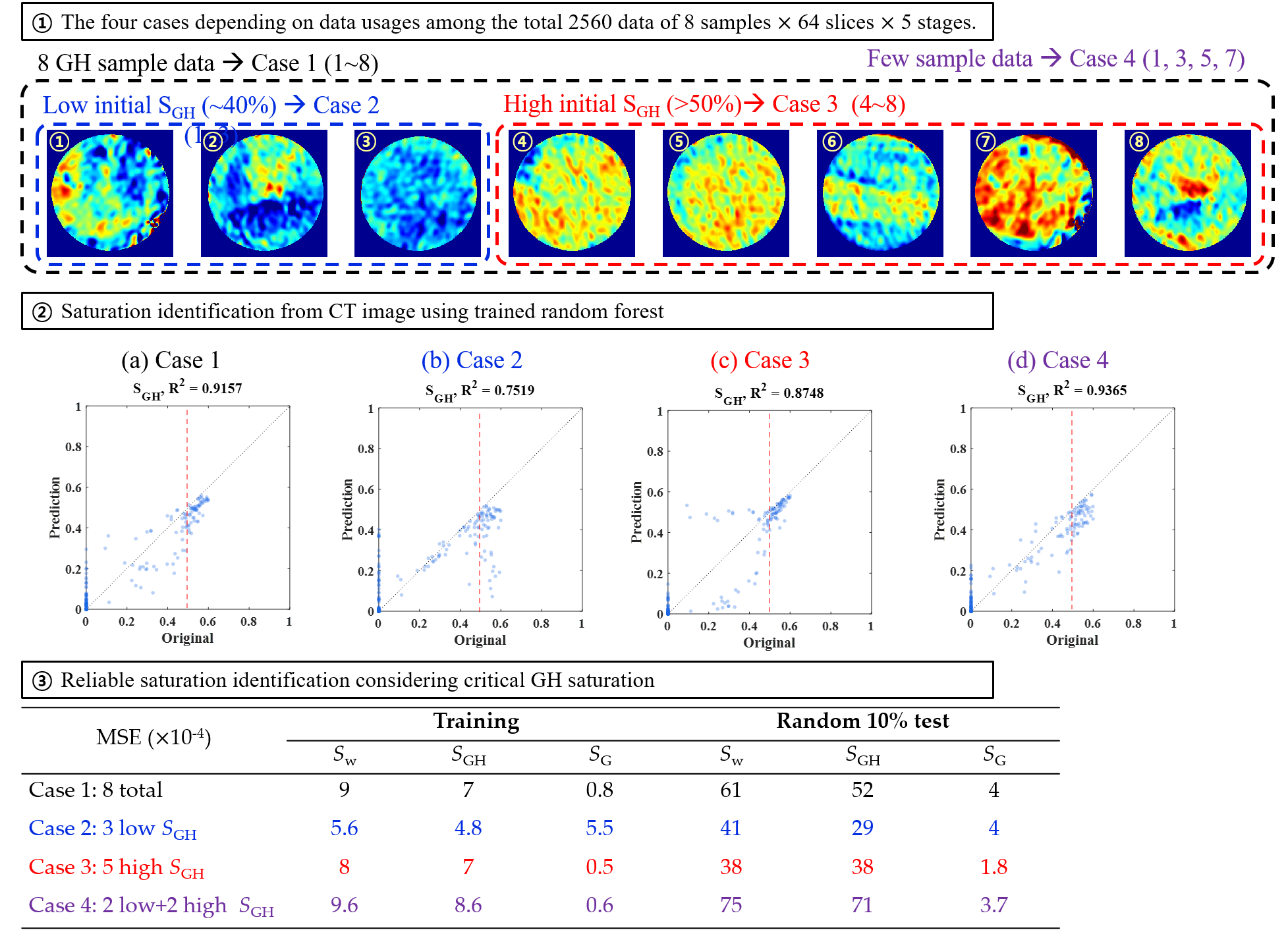
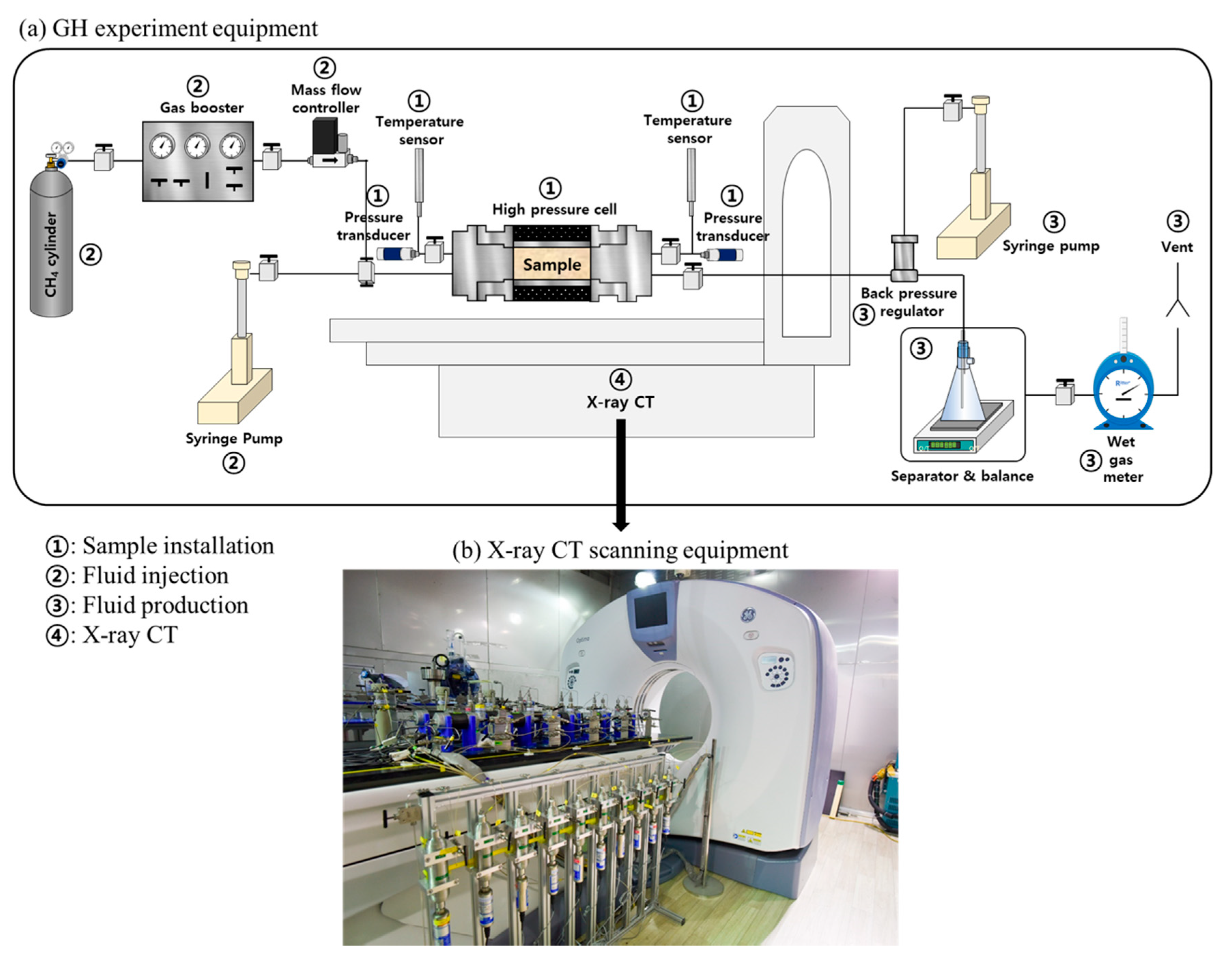
2.1. Experiments of Gas Hydrate (GH) with X-Ray Computerized Tomography (CT) Scanning

KIGAM introduced a visualization system to experiment with different GH production options and a variety of production-related parameters. The visualization system consists of four main parts: GH sample installation, fluid injection, fluid production, and X-ray CT equipment, as presented in Figure 1. X-ray CT scanning is continuously performed during all experimental procedures. The high-pressure cell is composed of glass fiber and aluminum complex to minimize X-ray diffraction, with a diameter and length of 1 and 2 inches, respectively (Figure 1a). The X-ray CT scanning equipment (General Electricity OPTIMA 660) can scan at a rate of up to 96 mm/sec and can also conduct quantitative analysis. Other details about the equipment and its specifications are explained in Kim et al. [16].

In this study, GH generation is followed by GH sample charge, initial water saturation setting, and pressurization by CH₄. In particular, the pressurization is performed by excess gas method, which forms GH showing grain-coating or cementing-type habit [32,33]. Excess gas method is to increase pressure and decrease temperature by methane gas injection in partial water saturation condition. As presented in Figure 2, the experiment consists of five stages before the GH depressurization stage: “DRY”, “SAT”, “IWS”, “GH”, and “GTW”, described as follows. X-ray CT was scanned for every stage and the scanned CT images corresponded to the five stages. Only one scan is sufficient to determine the internal state of a target GH sample in each of the five stages because there is no critical change within the same stage. In the DRY stage, CT images are scanned immediately after the charge with sand to check whether the distribution of sand particles is regular and that those CT values are smallest for the entire experiment because a sand sample is saturated only with the air. Before SAT stage, the entire experiment system is inspected to ensure that the system is stably operated and each compartment is tightly connected through valves. In the SAT stage, a GH sample is 100% saturated with water, which has the largest CT values in this experiment. Therefore, the smallest and largest CT values are utilized to both normalize and quantitatively analyze CT images, as follows:

$$C{T}_{norm}=\frac{C{T}_{STAGE}-C{T}_{DRY}}{C{T}_{SAT}-C{T}_{DRY}},$$

(1)

where $C{T}_{norm}$ is the normalized CT value; $C{T}_{STAGE}$ is the CT value from the IWS, GH, or GTW stages. Note that more experimental explanation can be reviewed in detail in [16].

In the IWS stage, the sample has initial water saturation with CH₄, wherein the GH sample is pressurized to make GH (GH stage of Figure 2d). Methane gas is injected with air-cooling operation until it reaches the suitable high pressure and low temperature condition for GH formation. Then, remaining gas in the GH sample is replaced by 3% salinity brine to build the most similar environment of naturally reserved GH (GTW stage of Figure 2e). According to Equation (1), the normalized CT values will be 0 and 1 for the images from the DRY and SAT stages, respectively. In terms of the IWS, GH, or GTW stages, the normalized CT values will be between 0 and 1.

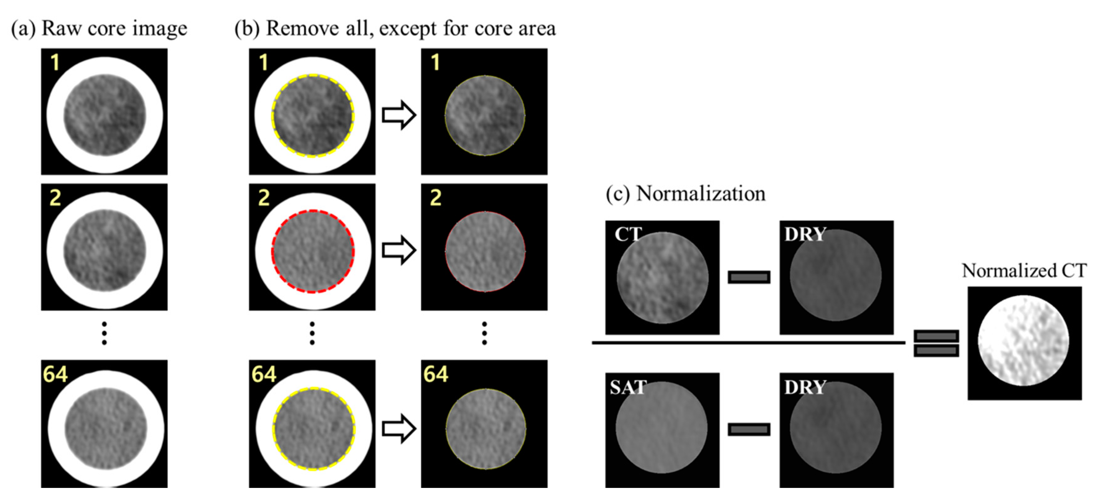
2.2. Data Acquisition and Preprocessing

The CT images resolution is 512 $\times$ 512 $\times$ 96 and the size of each pixel is ~660 µm and 100 µm in the vertical and horizontal directions, respectively. High CT values due to the end-piece, including the temperature sensor, were removed in order to acquire proper CT values for training the machine-learning models. Thus, a total of 96 slices were obtained; however, only the front 64 slices were utilized as training data. According to Equation (1), given CT values were normalized and the related procedures are shown in Figure 3. Row CT images were obtained by CT scanning (Figure 3a) and the useless parts were discarded (Figure 3b). Target images for normalization were put to the CT slot as described in Figure 3c and this procedure makes image data standardized for versatility between other GH sample experiments. Finally, the normalized CT images and three phase saturations comprised the data pairs for input and output of training data, respectively.

Saturation values of water, GH, and gas were generated, corresponding to the normalized GH CT images, a process known as “labeling” for building training data for supervised learning [34]. CT images of the DRY and SAT stages technically have fixed values such as S_G = 1 or S_W = 1, respectively. The IWS and GH stages would clearly show S_GH = 0 or S_W = 0, respectively. In addition, S_GH of the GTW stage would be the same as that of the GH stage. We can calculate three phase saturations according to those conditions, given an experimental environment according to

Table 1. Saturation and density conditions for labeling in the three experimental stages.

Experimental Stage	SW (Density, g/cc)	SGH (Density, g/cc)	SG (Density, g/cc)
“IWS” (14.7 psi, 18 °C)	SW,IWS (dW,IWS = 1)	SGH,IWS = 0	1 − SW,IWS (dG,IWS = 0.000678)
“GH” (2500 psi, 16 °C)	SW,GH = 0	SGH,GH (dGH,GH = 0.91)	1 − SGH,GH (dG,GH = 0.143)
“GTW” (2900 psi, 16 °C)	SW,GTW (dW,GTW = 1.008)	SGH,GTW = SGH,GH	1 − SW,GTW − SGH,GTW (dG,GTW = 0.167)

and Equations (2) and (3):

$$S_{\mathrm{W},\mathrm{STAGE}}\times d_{\mathrm{W},\mathrm{STAGE}}+S_{\mathrm{GH},\mathrm{STAGE}}\times d_{\mathrm{GH},\mathrm{STAGE}}+S_{\mathrm{G},\mathrm{STAGE}}\times d_{\mathrm{G},\mathrm{STAGE}}=C{T}_{\mathrm{norm}}^{\mathrm{avg}},$$

(2)

$$C{T}_{\mathrm{norm}, j}^{\mathrm{avg}}=\frac{1}{n_{\mathrm{c}}}{\sum }_{i=1}^{n_{\mathrm{c}}}C{T}_{\mathrm{norm},j, i} \mathrm{for} j=1,\dots ,n_{\mathrm{s}} ,$$

(3)

where $S$ and $d$ indicate saturation and density, respectively. The subscripts $\mathrm{W}$, $\mathrm{GH}$, and $\mathrm{G}$ of $S$ are water, gas hydrate, and gas, respectively. The second subscript $\mathrm{STAGE}$ represents the given experimental stage (IWS, GH, or GTW). $C{T}_{\mathrm{norm}}^{\mathrm{avg}}$ is the average, normalized CT value from all data pixels ($n_c$) of the actual GH sample in one slice image (i.e., the circle-shaped area in the right column of Figure 3b). Here, $n_{\mathrm{c}}$ is 47,992 at the experimental environment in this study. $n_{\mathrm{s}}$ is the number of slices of a GH sample; 64 in this experiment setting. Consequently, one CT slice image is paired with three saturation values, becoming one sample for training data.

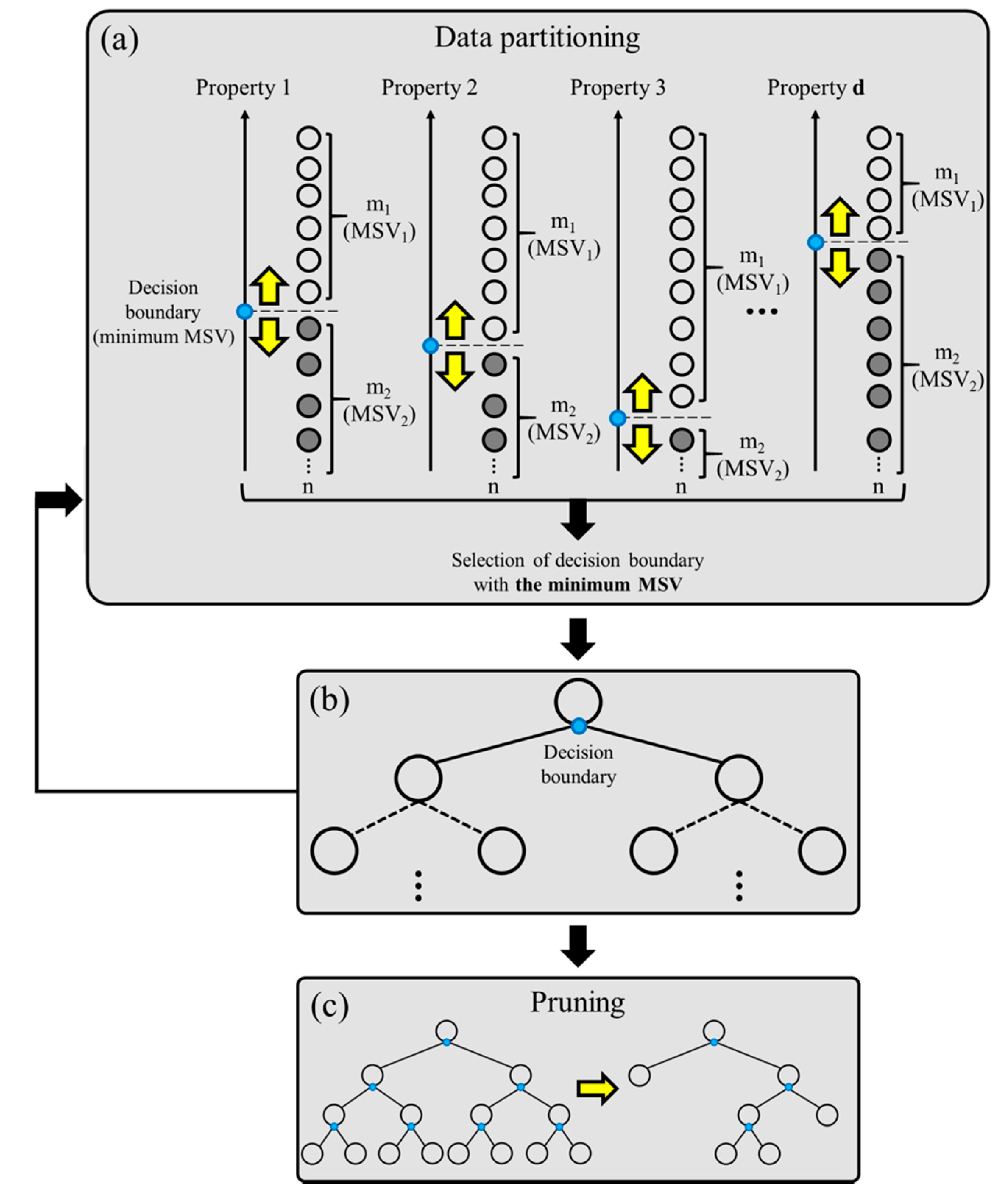
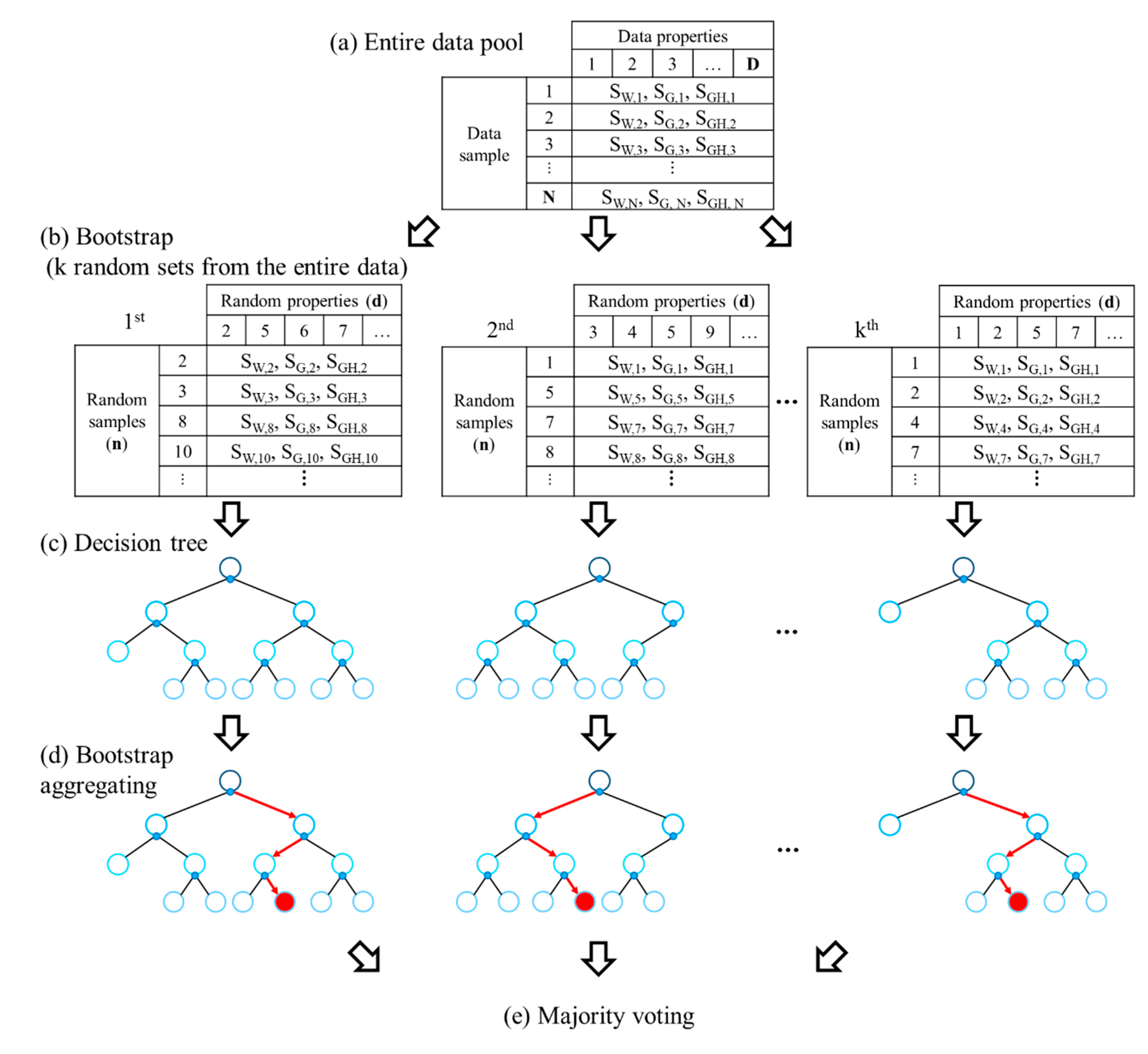
2.3. Machine-Learning Methodology: Random Forest (RF)

As an ensemble machine-learning method, RF consists of multiple decision trees. Figure 4 describes how a decision tree is constructed when it has n sample data of the property of d. First, the data portioning procedure divides the given data into m₁ and m₂, locating the single decision boundary which minimizes the average of two mean square variances, MSV₁ and MSV₂ (Figure 4a). The decided boundary then becomes a standard for dividing into two branches (Figure 4b). This procedure is repeated until reaching a specific criterion, which is usually set by a user. After that, pruning is conducted to prevent the final decision tree from overfitting (Figure 4c).

Figure 5 shows RF composed of multiple decision trees. First, subsequent multiple data groups (k) are constructed by random selection from the entire data pool, known as bootstrapping (Figure 5b). Each decision tree (Figure 4) is then trained according to the multiple data groups (Figure 5c), yielding different looks due to the different data compositions from bootstrapping. In bootstrap aggregating, an output (saturation) is estimated based on where the given value (normalized CT image) is assigned to (Figure 5d,e), indicated according to the multiple decision trees. According to the principle of RF, the larger the number of decision trees, the more stable the performance shown by RF. Typically, the number of decision trees is set on the level of a couple of hundreds, at most thousands. Under the circumstances of given computing power (Intel Xeon Gold 6136 central processing unit with 3 and 2.99 GHz processors and 128 GB random-access memory), a couple of hundred trees is sufficiently affordable. Besides, the computational cost issue is out of scope from this study. Therefore, that issue will not be handled in detail.

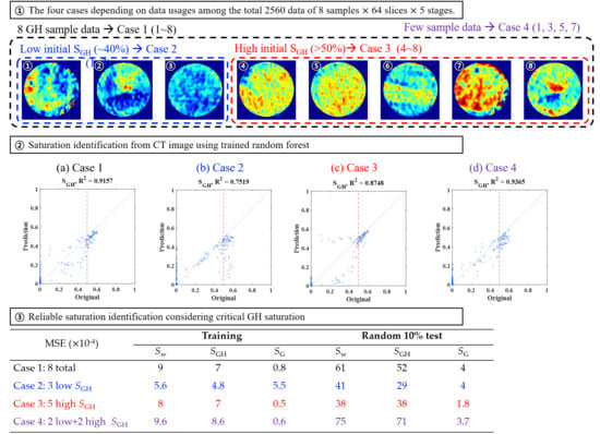
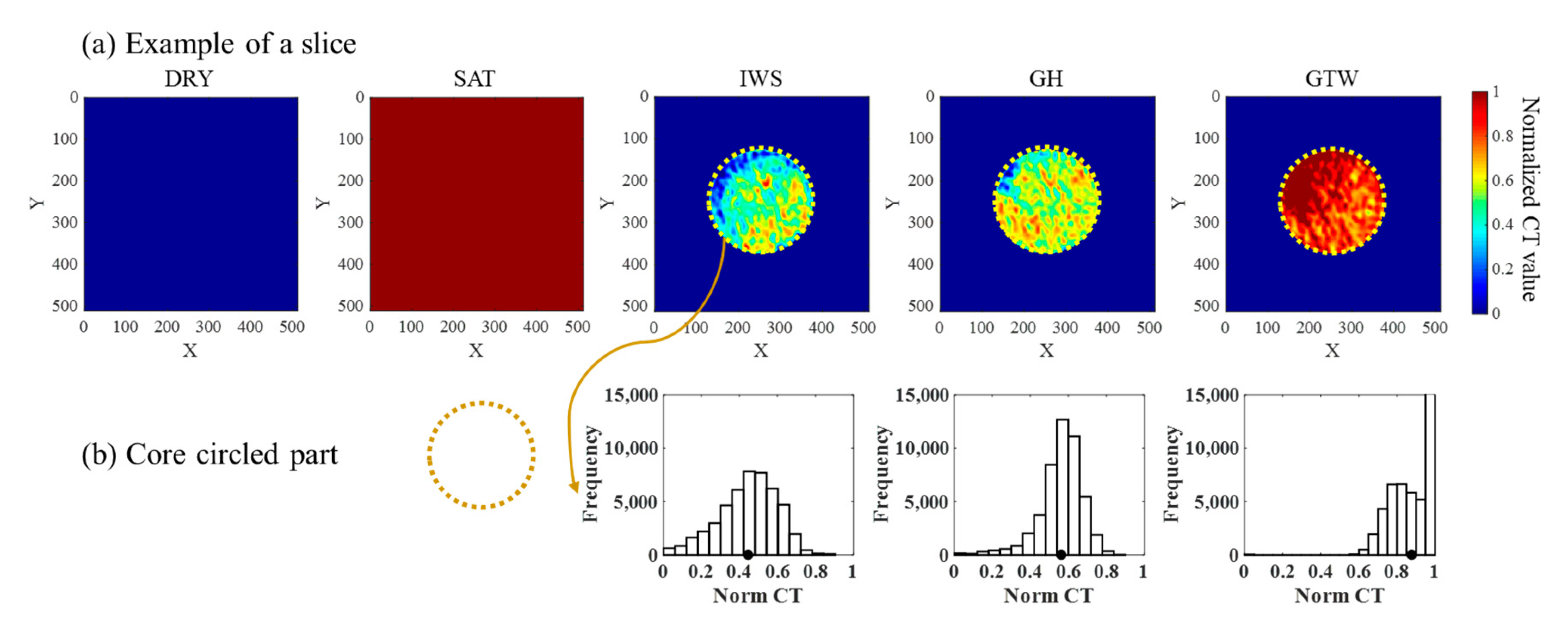
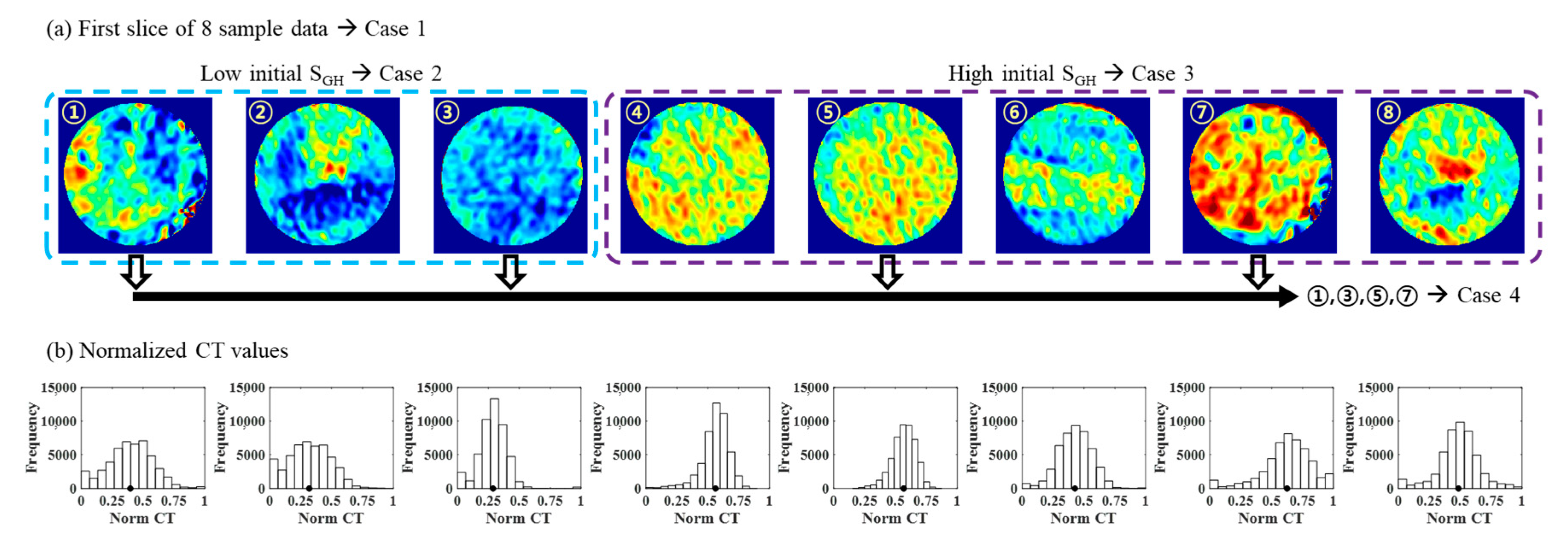
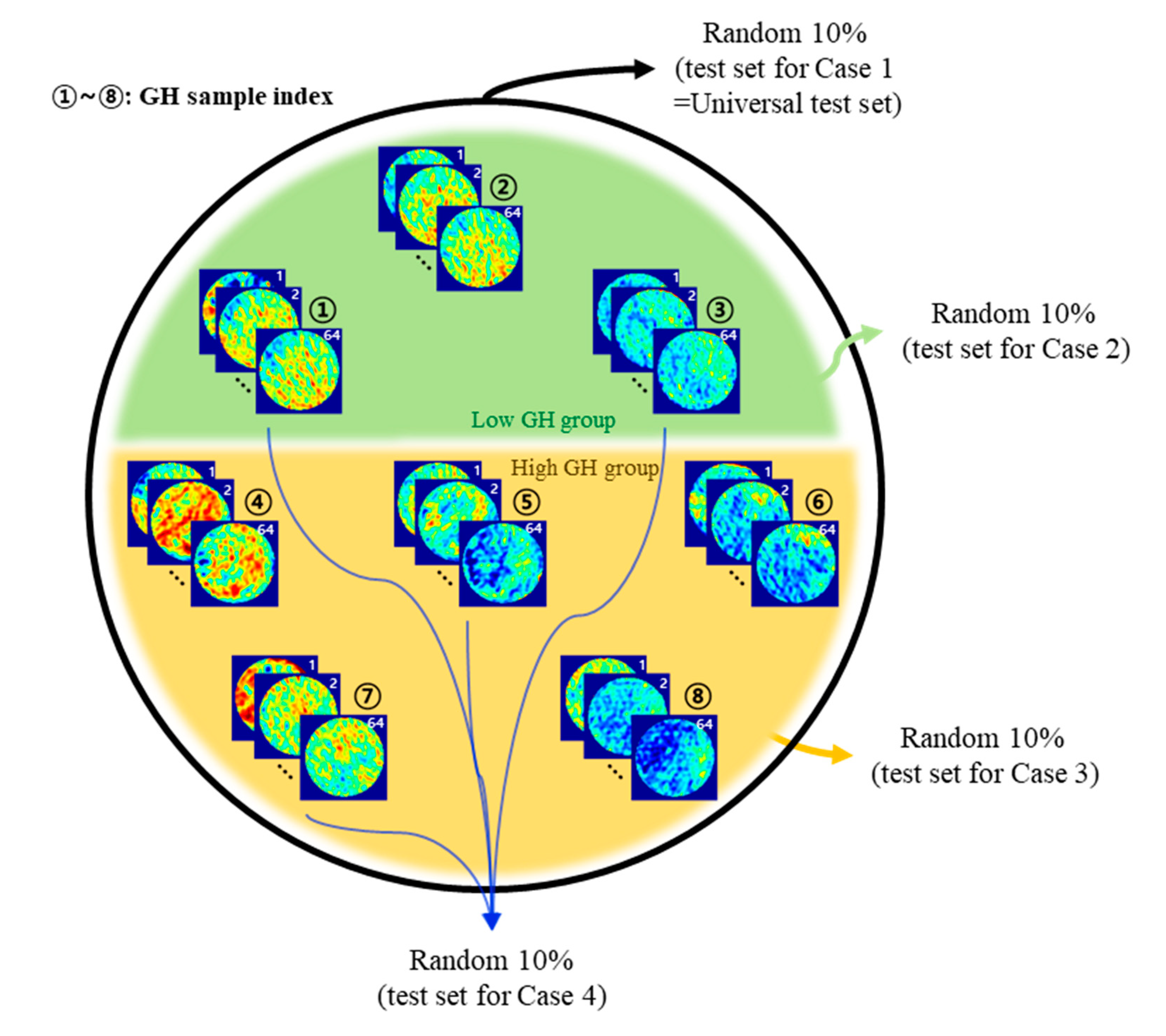
3. Construction of Training Data

Figure 6 shows an example of normalized CT values and their distribution in the five experimental stages. In the DRY and SAT stages, only 0 or 1 values are present for all normalized CT values according to Equation (1) and Figure 3 [16]. On the contrary, individual distributions in the IWS, GH, and GTW stages are present, shown in histogram form as Figure 6b. The GH sample is marked with the yellow dotted circles in three of the stages and each histogram covers only that circle area. From IWS to GTW, the averaged, normalized CT values become larger than the previous stage because the overall density increases corresponding to the experiment design due to the five stages (Figure 2). The normalized CT values become closer to 0.9–1, similar to the density of GH and water (Table 1).

Figure 7 describes the eight total GH samples for the experiment and their distributions of normalized CT values of the GH stage. The first to third samples are categorized into the low GH saturation group, while the fourth to eighth samples are assigned to the high GH saturation group. There was no difficulty with the separation into these two groups because of the obvious difference of S_GH values—whereby values were around 40% and 50%, respectively. Figure 7b presents the distributions of normalized CT values for the first slice of eight GH samples, with black dots indicating the means of each distribution. Generally, the low GH saturation group has low averages of the normalized CT values and the high GH saturation group gives higher average values. We can distinguish S_GH values into the forty- and fifty-percent groups which are taken as the conventional values and critical values, respectively, because S_GH,C was expected to be ~50% for the target GH sample in this study. For values close to that of S_GH,C, production efficiency of GH can be drastically reduced due to the slow pressure propagation in porous media.

The eight GH samples are randomly indexed after they are categorized into the two groups. In this study, the total eight GH samples are divided into four cases (Cases 1–4) for analysis of data construction and machine-learning performance. Case 1 represents the total eight GH samples and Cases 2 and 3 are the low and high S_GH, respectively. Case 4 consists of the odd-numbered GH samples—1, 3, 5, and 7—for randomly constructed data collection with low and high S_GH evenly. Case 4 is set to have the four selected GH samples in order to produce the fairest comparison with Cases 2 and 3 by fitting to the amount of training data.

Table 2. Gas hydrate (GH) saturation and computerized tomography (CT) values in the “GH” stage for eight GH samples.

shows averaged GH saturation and CT values of each GH sample and Cases 1–4. Orange-colored cells indicate the utilized GH sample for each of the four cases. The means that Cases 1 and 4 are similar to each other because they are composed of combined GH samples from the low and high S_GH groups. The difference between averaged S_GH of Cases 2 and 3 is ~11%, which could give significant contrast of GH behaviors.

Figure 8 and

Table 3. Conditions and settings for Cases 1–4 with random forest.

Method	List	Case 1	Case 2	Case 3	Case 4
Number of data	Entire data	2560	960	1600	1280
	Training data	2304	864	1440	1152
	Test data (10% of the entire data)	256	96	160	128
Training condition of RF	Maximum depth	10
	Number of trees	200
	Number of properties	219
	Data size of one sample	47,996

explain how the training and test data are divided and constructed for Cases 1–4. Figure 8 illustrates that four test sets are randomly selected from each data pool as a conventional machine-learning procedure. Case 1 uses all eight GH samples, and its test set consists of a random 10% of these. This test set of Case 1 is set as the universal test set, which is utilized as the common standard to compare all four cases with each other. The test sets for Cases 2, 3, and 4 are random 10% sets from each entire pool, represented by green, orange, and blue colored lines, respectively, in the figure. Training of RF is conducted for all four cases and the number of used training data is presented in Table 3. The eight GH samples have 320 data points due to the multiplication of 5 stages and 64 slices (Figure 2 and Figure 3). Case 1 has 2560 due to the multiplication of 8 GH samples and 320 slices. The number of training data should then be 2304, which is 2560 subtracted by 256, and the same procedure is carried out for the rest of the three cases. The detailed training conditions of RF are shown in Table 3. Regarding number of properties, 219 is determined by the root of the total number of CT values, 47,996.

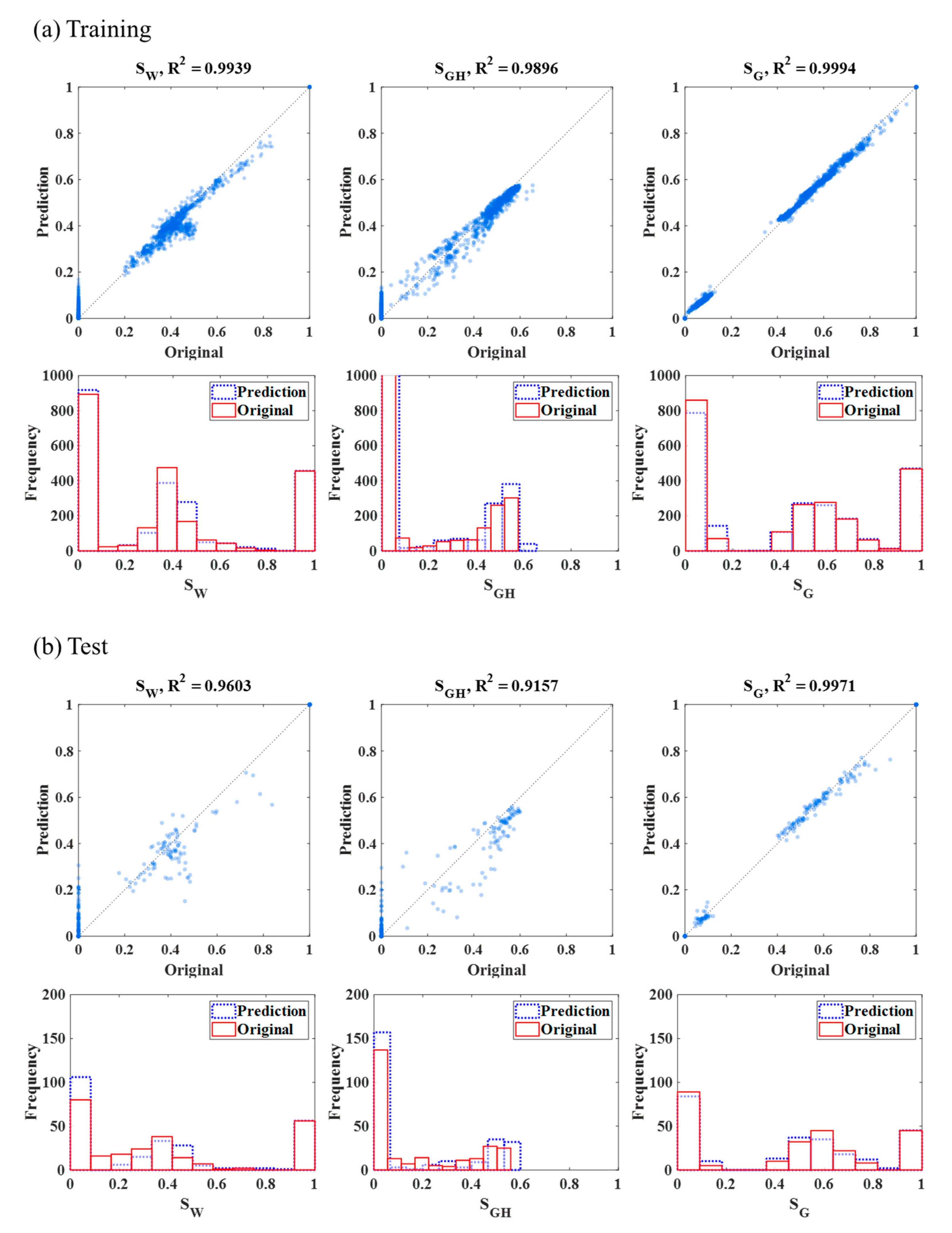
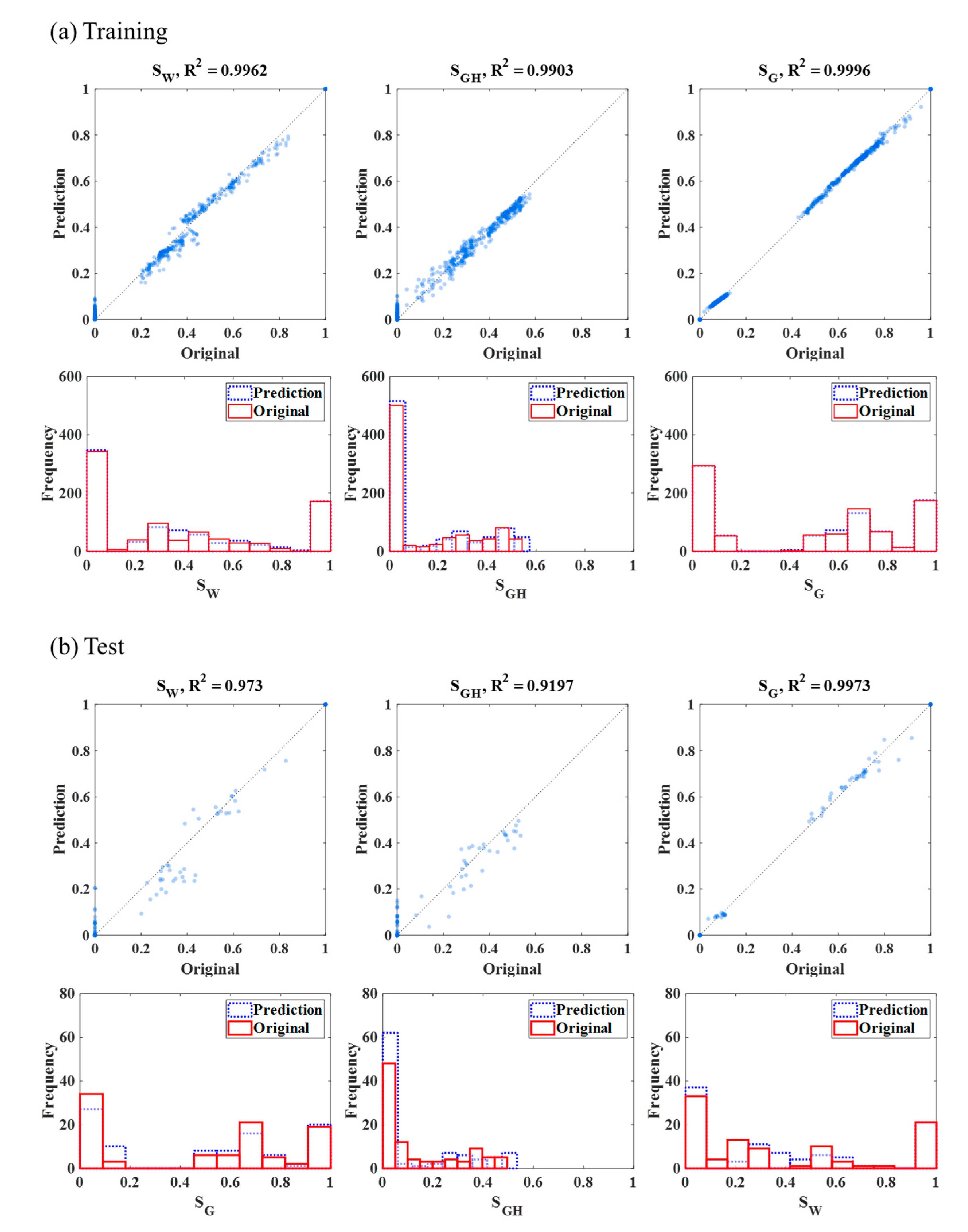
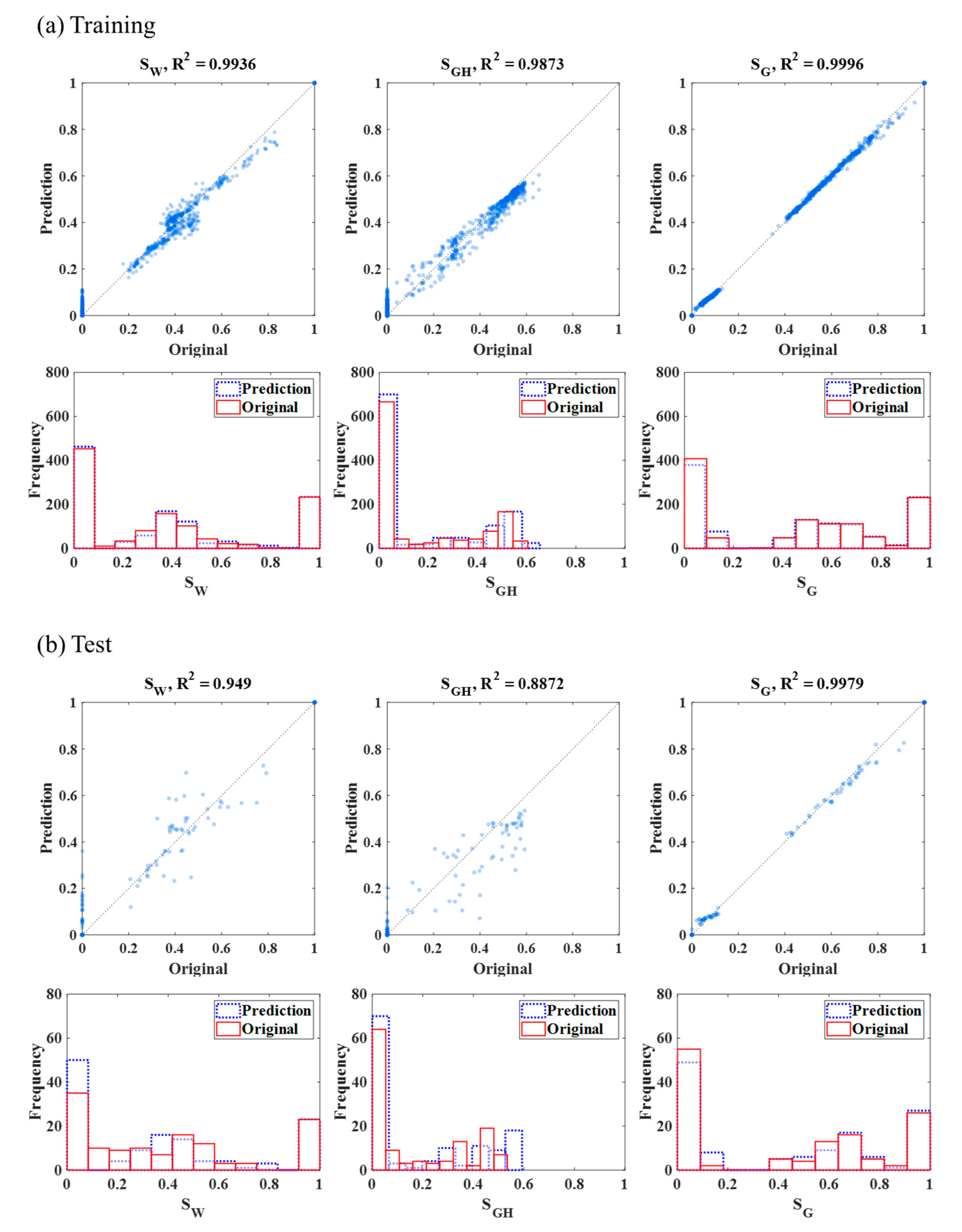
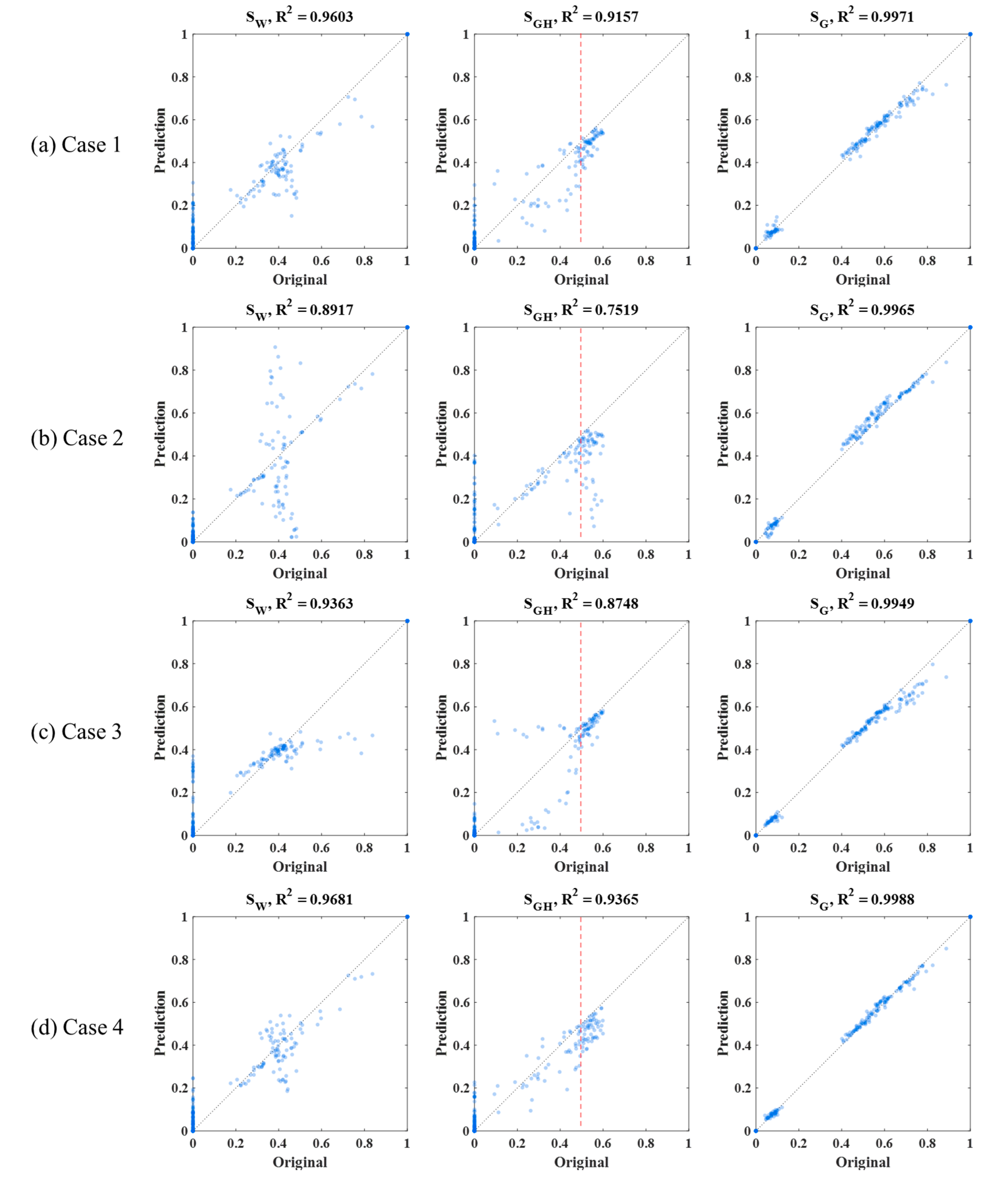
4. Results and Discussion

Figure 9, Figure 10, Figure 11 and Figure 12 are the results of RF for the training and test sets, respectively. Figure 9a, Figure 10a, Figure 11a and Figure 12a are the training and Figure 9b, Figure 10b, Figure 11b and Figure 12b are the test set, while each column lists S_W, S_GH, and S_G in order. In both (a) and (b) panels, the first row is the scatterplot and the second row displays the same results in a histogram. In the first row, the X-axis indicates the original value of saturations and the Y-axis indicates the predicted (modeled) values. Blue dots indicate individual data samples and increasing darkness of the color indicates increasingly scattered data relative to a certain position. Therefore, although some of data seem to be deviated from the diagonal line, it can give a high coefficient of determination (S_W of Figure 9b). Correlation coefficients are calculated and presented at the top of all charts. In the histograms of the second row, the blue dotted box means the predicted saturation values and the red solid-line box presents the original saturations.

Figure 9 illustrates the largest number and widest range of data because all eight GH samples are included. The coefficient of determination (R²) of the training data is ~0.99 for all of the variables—S_W, S_GH, and S_G. In particular, S_G shows considerable fitting between the original and the predicted values in comparison with S_W and S_GH. This is because the density of water and GH are relatively similar, which leads to little difference in X-ray CT images and normalized CT values. However, the density of gas is much lower than that of water or GH, thereby causing certain changes in CT values. The certain difference of densities between gas and the others causes a clear discrepancy between normalized CT values of gas and the others. It makes the prediction of gas saturation easier than the prediction of water and GH saturations. This phenomenon was identified in our previous study [16].

Figure 10 and Figure 11 contrast each other in terms of S_GH. It was expected for these charts to show the different distribution of S_GH because they are separated with S_GH criteria, showing the S_GH results. In both Cases 2 and 3, the overall machine-learning performances are suitable considering that all R² values are greater than 0.99 and the scattered dots are positioned on the diagonal line in an orderly fashion. However, in terms of S_GH, Case 2 has a relatively wide range of 0–0.6, whereas Case 3 mostly shows either 0 or ~0.5. In Figure 11, the scattered dots are deviated from the diagonal line especially near 0.4, which is a comparably low S_GH. It would be expected that Case 3 was trained for large S_GH values compared to Case 2, which is the reason why Case 3 functions this way according to the given data composition.

Figure 12 shows overall decent performance except for the test set of S_GH whose R² is 0.89, the lowest value. Case 1 has the smallest R² value of 0.92 in the test set for S_GH. In Cases 2 and 3, S_GH shows the smallest R², seemingly indicating that the most challenging component of the process is the identification of S_GH for the test sets. The density of water is maintained at approximately 1 g/cc regardless of experimental stage. However, the density of GH highly depends on the given pressure and temperature of the three experimental stages—IWS, GH, and GTW (i.e., the last column of Table 1). Therefore, S_GH differently affects the normalized CT values according to these experimental stages. This phenomenon of S_GH could further lead to more complex relationships between S_GH and the normalized CT values, and consequently, results in higher difficulty of the machine-learning training. For this reason, the methodology introduced in this study should continue to be conducted.

In Figure 13 and Figure 14, the four trained RF models correspond to the four cases, and those four RF models are tested using the universal test. The test results shown in Figure 13a and Figure 14a are identical with those of Figure 9b. In most machine-learning-related studies, its trained performance is mainly evaluated with errors and correlation coefficients between original and predicted data in the test data set. In this study, the four, learned, RF models are tested together with the universal test set for a consistent analysis. According to one previous study, it was estimated that S_GH,C might be somewhere between approximately 50–60% [31].

Interestingly, according to the S_GH results shown in Figure 13b,c, an obvious boundary is shown at ~50% S_GH, where the red dotted lines indicate the validation as to whether there is any trend related to S_GH,C. In Figure 13b, the S_GH values over 50% are poorly matched in performance compared to Figure 13a,c,d. On the other hand, to the left of the red line in the S_GH results shown in Figure 13b, the S_GH values less than 50% have comparatively good fitting results. This is further emphasized when viewing the left of the red line for S_GH results of Figure 13c.

Furthermore, it should be noted that Case 2 shows deviated results for over 50% S_GH (Figure 13b and Figure 14b), even though some training data nearby showed 50% S_GH (Figure 10a). This is an indication of an additional effect other than the range of training data values, “critical gas saturation”. Thus, we can expect certain distinguishing behaviors of GH samples according to the different S_GH,C values setting. Although there could be some S_GH values near 40% or 50% in one specific GH sample, the trend of GH behaviors would highly depend on the decided S_GH,C as an experimental condition. Based on that possibility, we can infer that there must be a certain radical change of GH behavior from S_GH,C, which is evaluated as ~50% in this study.

Cases 2, 3, and 4 are relatively comparable to each other in terms of the absolute number of training data—864, 1440, and 1152, respectively (Table 3)—all of which are close to the value of 1000. Considering this, Case 4 has relatively less-biased results of S_GH compared to Cases 2 and 3 (Figure 13d). On both the left and right sides of the red line, data are generally positioned following the diagonal line.

Table 4. Mean square error (MSE) of training and test sets for Cases 1–4.

$(\times {10}^{-4})$	Training			Random 10% Test				Universal Test
	Sw	SGH	SG	Sw		SGH	SG	Sw		SGH	SG
Case 1: 8 total	9	7	0.8	61		52	4	61		52	4
Case 2: 3 low SGH	5.6	4.8	5.5	41		29	4	170		143	5.5
Case 3: 5 high SGH	8	7	0.5	38		38	1.8	100		71	8
Case 4: 2 + 2 SGH	9.6	8.6	0.6	75		71	3.7	49		44	1.6
	Average of SW, SGH, and SG
Case 1: 8 total	5.6				39
Case 2: 3 low SGH	5.3				24.7				106.2
Case 3: 5 high SGH	5.2				25.9				60.0
Case 4: 2 + 2 SGH	6.3				49.9				31.5

organizes the mean square error (MSE) results of Cases 1–4 for both the training and test sets and the universal test set. The MSEs are computed as follows:

$$MSE=\frac{1}{n}{\sum }_{i=1}^n{\left(Ori{g}_i-Pre{d}_i\right)}^2,$$

(4)

where $n$ is the number of training or test data, $Ori{g}_i$ is the original ith data, and $Pre{d}_i$ represents the predicted data for the ith original data.

Table 4 presents the MSEs corresponding to each data set, fluid phase, and case, and also shows the averaged MSEs for an overall comparison of training data, random 10% data, and the universal test. In terms of each fluid phase, S_G has the lowest errors among the three phase saturations. As shown in Figure 9, Figure 10, Figure 11 and Figure 12 and Figure 13, S_W and S_GH have the larger MSEs. As conventional machine-learning shows, the MSEs of the training data are lower than those of the two test sets.

Meaningful lessons can be understood from the comparison between all four cases. First, the absolute number of data substantially affects machine-learning performance (Cases 1 and 4). Typically, a higher number of training data would be expected to have better performance, as long as other conditions such as features and algorithms are sufficiently appropriate [35,36]. However, Cases 1 and 4 have two times the difference in the number of data; however, the MSEs are nearly in the same scale without critical difference (39 and 31.5 in the universal test). Therefore, the results of Cases 1 and 4 of this study indicate that distributions of these cases must be similar to each other, such that they also produce similar-scaled MSEs. This indicates that the process of how data is constructed is as important as the absolute number of data for machine-learning performance. Second, if it were possible to obtain a limited number of data, it would be ideal to focus on the specific S_GH range. Cases 2 and 3 show lower MSEs compared to Cases 1 and 4 in random 10% test with the similar number of training data, which means specialized targeted data construction can be strategically advantageous for machine-learning performance. Third, the ratio of MSEs from Cases 2 and 3 is about 5:3, which is similar to a ratio of the rest of the data for Cases 2 and 3, respectively—in that, Case 2 has only three GH samples among the total eight GH samples and the rest has five GH samples. For Case 3, the rest of the data has three GH samples. The less related the data, the larger the MSE.

5. Conclusions

This paper proposed the saturation identification of water, GH, and the gas phase in GH samples based on a machine-learning method in consideration of S_GH,C. Moreover, the effects of training data quantity and quality were analyzed for RF utilization in the four cases. Compared to our previous related study [16], this study utilized five additional GH samples, whose number of data was 1600. Owing to this extra data, we could categorize samples into low and high S_GH groups and determine how the number of data and S_GH,C affect the overall machine-learning performance.

This study validated the significant influence of S_GH,C in cases where training data consists of low and high S_GH groups. The average MSE differences of random 10% test (Table 4) between Cases 1 and 4 (10.9) was larger than that between Cases 2 and 3 (1.2), indicating that S_GH can be a highly important standard for saturation identification in GH formation and dissociation experiments. In particular, S_GH,C can be an important criterion to divide training data when any machine-learning technique is applied to given CT images in a GH experiment (refer to Cases 2 and 3). Thus, the separation of CT images according to S_GH,C can be an appropriate option for constructing training data, leading to obtaining reliably specialized machine-learning models.

In conclusion, it is important to acquire a sufficiently high number of data in order to carry out trustworthy application of machine-learning; however, proper data construction should also be considered. It was expected that one specific standard for data building would be identified from the essential factors of interested behaviors based on domain knowledge, and it was verified to be S_GH,C from this study. Therefore, if obtainment of data was restricted to some specific type or quantity of data, the first order of business would be selection of GH experiment to be conducted first according to a value of S_GH. After that, GH experiments could be intensively performed to preferentially obtain data of CT images and saturations based on a target field condition of S_GH,C. Accordingly, S_GH,C would be the optimal guideline for training data building.

In future studies, additionally acquired GH CT images would be assigned to one of low or high S_GH groups whose criterion is S_GH,C. According to that, two machines could then be trained with those two categorized data, respectively, so as to produce two customized machine-learning models. After construction of the reliable machine-learning models based on qualitatively and quantitatively sufficient data, those models could be utilized to identify saturation values during the dissociation stage of GH sample experiments with depressurization. Saturation identification of GH samples in real time is expected to be a powerful tool to help determine general GH behaviors and conduct a variety of experiments for optimization of the parameters of GH production by depressurization.

References

1. Kumar, P.; Collett, T.S.; Shukla, K.M.; Yadav, U.S.; Lall, M.V.; Vishwanath, K.; Yamada, Y. India National Gas Hydrate Program Expedition-02: Operational and technical summary. Mar. Petrol. Geol. 2019, 108, 3–38. [Google Scholar] [CrossRef]
2. Li, J.; Ye, J.; Qin, X.; Qiu, H.J.; Wu, N.Y.; Lu, H.L.; Xie, W.W.; Lu, J.A.; Peng, F.; Xu, Z.Q.; et al. The first offshore natural gas hydrate production test in South China Sea. China Geol. 2018, 1, 5–16. [Google Scholar] [CrossRef]
3. Haines, S.S.; Hart, P.E.; Collett, T.S.; Shedd, W.; Frye, M.; Weimer, P.; Boswell, R. High-resolution seismic characterization of the gas and gas hydrate system at Green Canyon 955, Gulf of Mexico, USA. Mar. Petrol. Geol. 2017, 82, 220–237. [Google Scholar] [CrossRef] [Green Version]
4. Chong, Z.R.; Yang, S.H.B.; Babu, P.; Linga, P.; Li, X.-S. Review of natural gas hydrates as an energy resource: Prospects and challenges. Appl. Energy 2016, 162, 1633–1652. [Google Scholar] [CrossRef]
5. Ito, T.; Komatsu, Y.; Fujii, T.; Suzuki, K.; Egawa, K.; Nakatsuka, Y.; Konno, Y.; Yoneda, J.; Jin, Y.; Kida, M.; et al. Lithological features of hydrate-bearing sediments and their relationship with gas hydrate saturation in the eastern Nankai Trough, Japan. Mar. Petrol. Geol. 2015, 66, 368–378. [Google Scholar] [CrossRef]
6. Lee, J.Y.; Jung, J.W.; Lee, M.H.; Bahk, J.J.; Choi, J.; Ryu, B.J.; Schultheiss, P. Pressure core based study of gas hydrates in the Ulleung Basin and implication for geomechanical controls on gas hydrate occurrence. Mar. Petrol. Geol. 2013, 47, 85–98. [Google Scholar] [CrossRef]
7. Huh, D.; Lee, J.Y. Overview of gas hydrates R&D. J. Korean Soc. Miner. Energy Resour. Eng. 2017, 54, 201–214. [Google Scholar]
8. Boswell, R.; Schoderbek, D.; Collett, T.S.; Ohtsuki, S.; White, M.; Anderson, B.J. The Iġnik Sikumi field experiment, Alaska North Slope: Design, operations, and implications for CO2-CH4 exchange in gas hydrate reservoirs. Energy Fuel. 2017, 31, 140–153. [Google Scholar] [CrossRef]
9. Koh, D.Y.; Kang, H.; Lee, J.W.; Park, Y.; Kim, S.J.; Lee, J.; Lee, J.Y.; Lee, H. Energy-efficient natural gas hydrate production using gas exchange. Appl. Energy 2016, 162, 114–130. [Google Scholar] [CrossRef]
10. Zhao, J.; Zhu, Z.; Song, Y.; Liu, W.; Zhang, Y.; Wang, D. Analyzing the process of gas production for natural gas hydrate using depressurization. Appl. Energy 2015, 142, 125–134. [Google Scholar] [CrossRef]
11. Anderson, B.J.; Kurihara, M.; White, M.D.; Moridis, G.J.; Wilson, S.J.; Pooladi-Darvish, M.; Gaddipati, M.; Masuda, Y.; Collett, T.S.; Hunter, R.B.; et al. Regional long-term production modeling from a single well test, Mount Elbert Gas Hydrate Stratigraphic Test Well, Alaska North Slope. Mar. Petrol. Geol. 2011, 28, 493–501. [Google Scholar] [CrossRef]
12. Tang, L.G.; Li, X.S.; Feng, Z.P.; Li, G.; Fan, S.S. Control mechanisms for gas hydrate production by depressurization in different scale hydrate reservoirs. Energy Fuel. 2007, 21, 227–233. [Google Scholar] [CrossRef]
13. Lee, M.; Suk, H.; Lee, J.; Lee, J. Quantitative analysis for gas hydrate production by depressurization using X-ray CT. In Proceedings of the 2018 Joint International Conference of the Geological Science & Technology of Korea, KSEEG, Busan, Korea, 17–20 April 2018; p. 363. [Google Scholar]
14. Wang, J.; Zhao, J.; Yang, M.; Li, Y.; Liu, W.; Song, Y. Permeability of laboratory-formed porous media containing methane hydrate: Observations using X-ray computed tomography and simulations with pore network models. Fuel 2015, 145, 170–179. [Google Scholar] [CrossRef]
15. Mikami, J.; Masuda, Y.; Uchida, T.; Satoh, T.; Takeda, H. Dissociation of natural gas hydrate observed by X-ray CT scanner. Ann. N. Y. Acad. Sci. 2006, 912. [Google Scholar] [CrossRef]
16. Kim, S.; Lee, K.; Lee, M.; Ahn, T.; Lee, J.; Suk, H.; Ning, F. Saturation modeling of gas hydrate using machine learning with X-ray CT images. Energies 2020, 13, 5032. [Google Scholar] [CrossRef]
17. Alhashem, M. Supervised machine learning in predicting multiphase flow regimes in horizontal pipes. In Proceedings of the Abu Dhabi International Petroleum Exhibition & Conference, Abu Dhabi, UAE, 11–14 November 2019. [Google Scholar] [CrossRef]
18. Singh, A.; Ojha, M.; Sain, K. Predicting lithology using neural networks from downhole data of a gas hydrate reservoir in the Krishna-Godavari basin, eastern Indian offshore. Geophys. J. Int. 2020, 220, 1813–1837. [Google Scholar] [CrossRef]
19. Kim, S.; Kim, K.H.; Min, B.; Lim, J.; Lee, K. Generation of synthetic density log data using deep learning algorithm at the Golden field in Alberta, Canada. Geofluids 2020, 2020, 5387183. [Google Scholar] [CrossRef] [Green Version]
20. Kim, S.; Lee, K.; Lim, J.; Jeong, H.; Min, B. Development of ensemble smoother-neural network and its application to history matching of channelized reservoir. J. Petrol. Sci. Eng. 2020, 191, 107159. [Google Scholar] [CrossRef]
21. Kim, S.; Min, B.; Kwon, S.; Chu, M. History matching of a channelized reservoir using a serial denoising autoencoder integrated with ES-MDA. Geofluids 2019, 2019, 3280961. [Google Scholar] [CrossRef]
22. Kim, S.; Min, B.; Lee, K.; Jeong, H. Integration of an iterative update of sparse geologic dictionaries with ES-MDA for history matching of channelized reservoir. Geofluids 2018, 2018, 1532868. [Google Scholar] [CrossRef] [Green Version]
23. Chen, B.; Harp, D.R.; Lin, Y.; Keating, E.H.; Pawar, R.J. Geologic CO2 sequestration monitoring design: A machine learning and uncertainty quantification based approach. Appl. Energy 2018, 225, 332–345. [Google Scholar] [CrossRef]
24. Esmaili, S.; Mohaghegh, S.D. Full field reservoir modeling of shale assets using advanced data-driven analytics. Geosci. Front. 2016, 7, 11–20. [Google Scholar] [CrossRef] [Green Version]
25. Lee, K.; Lim, J.; Yoon, D.; Jung, H. Prediction of shale gas production at Duvernay Formation using deep-learning algorithm. SPE J. 2019, 24, 2423–2437. [Google Scholar] [CrossRef]
26. Kim, J.; Kim, S.; Park, C.; Lee, K. Construction of prior models for ES-MDA by a deep neural network with a stacked autoencoder for predicting reservoir production. J. Petrol. Sci. Eng. 2020, 187, 106800. [Google Scholar] [CrossRef]
27. LeCun, Y.; Bottou, L.; Bengio, Y.; Haffner, P. Gradient-based learning applied to document recognition. Proc. IEEE 1998, 86, 2278–2324. [Google Scholar] [CrossRef] [Green Version]
28. Kim, T.; Kim, S.; Lim, J. Modeling and prediction of slug characteristics utilizing data-driven machine-learning methodology. J. Petrol. Sci. Eng. 2020, 195, 107712. [Google Scholar] [CrossRef]
29. Such, F.P.; Peri, D.; Brockler, F.; Hutkowski, P.; Ptucha, R.; Alaris, K. Fully convolutional networks for handwriting recognition. In Proceedings of the 2018 16th International Conference on Frontiers in Handwriting Recognition (ICFHR), Niagara Falls, NY, USA, 5–8 August 2018; pp. 86–91. [Google Scholar] [CrossRef] [Green Version]
30. Gil, S.M.; Shin, H.J.; Lim, J.S.; Lee, J. Numerical analysis of dissociation behavior at critical gas hydrate saturation using depressurization method. J. Geophys. Res. Sol. Ea. 2019, 124, 1222–1235. [Google Scholar] [CrossRef]
31. KIGAM. Gas Hydrate Exploration and Production Study; GP2016-027-2017(2); KIGAM: Daejeon, Korea, 2017; pp. 164–199. [Google Scholar]
32. Ta, X.H.; Yun, T.S.; Muhunthan, B.; Kwon, T. Observations of pore-scale growth patterns of carbon dioxide hydrate using X-ray computed microtomography. Geochem. Geophys. Geosyst. 2015, 16, 912–924. [Google Scholar] [CrossRef]
33. Waite, W.F.; Santamarina, J.C.; Cortes, D.D.; Dugan, B.; Espinoza, D.N.; Germaine, J.; Jang, J.; Jung, J.W.; Kneafsey, T.J.; Shin, H.; et al. Physical properties of hydrate-bearing sediments. Rev. Geophys. 2009, 47, RG4003. [Google Scholar] [CrossRef]
34. LeCun, Y.; Bengio, Y.; Hinton, G. Deep learning. Nature 2015, 521, 436–444. [Google Scholar] [CrossRef] [PubMed]
35. Domingos, P. A few useful things to know about machine learning. Commun. ACM 2012, 55, 78–87. [Google Scholar] [CrossRef] [Green Version]
36. Kang, B.; Lee, K. Managing Uncertainty in Geological Scenarios Using Machine Learning-Based Classification Model on Production Data. Geofluids 2020, 2020, 8892556. [Google Scholar] [CrossRef]
Figure 1. (a) Schematic diagram of the gas hydrate (GH) visualization system at Korea Institute of Geoscience and Mineral Resources (KIGAM) [31]; (b) the installed X-ray computerized tomography (CT) equipment for the system [31].
Energies 13 05844 g001
Figure 2. Flow chart of the gas hydrate (GH) generation experiment with computerized tomography (CT) scanning for obtaining the machine-learning data. (a) A sand sample made in DRY stage; (b) water saturated sample in SAT stage; (c) gas and water saturated status in IWS stage; (d) GH generation by pressurization in GH stage; (e) water replaces gas in GTW stage.
Energies 13 05844 g002
Figure 3. Modification and normalization of the CT images using ImageJ software [16]. (a) Acquisition of raw core images from the first to the sixty-fourth slice; (b) editing given images to acquire the target circle area; (c) normalization with CT images of DRY and SAT for standardization.
Energies 13 05844 g003
Figure 4. Construction of a decision tree with recursive partitioning and pruning based on n sample data of the d property [16]. (a) Search for decision boundary to minimize data impurity; (b) make branches out with decision boundaries; (c) remove excessive branches according to user-set standard.
Energies 13 05844 g004
Figure 5. Random forest with multiple decision trees for the prediction of the target parameters [16]. (a) The whole data with properties of D and data sample of N; (b) random data choice to construct data groups of k; (c) generation of k multiple trees from each of data groups; (d) summation of decisions according to multiple trees; (e) final decision making for given input.
Energies 13 05844 g005
Figure 6. Normalized CT values in the first slice of the fourth GH sample presented with a color scale. (a) Normalized CT values for each experimental stage; (b) histogram of core circled part for the three experimental stages—IWS, GH, and GTW.
Energies 13 05844 g006
Figure 7. Normalized CT values of the eight GH samples in the “GH” stage for construction of the four cases. (a) Combination of the samples for each case; (b) normalized CT values of the first slice image in histogram.
Energies 13 05844 g007
Figure 8. Two test sets: random 10% test from each of the four cases and universal test set from the eight GH samples.
Energies 13 05844 g008
Figure 9. (a) Training and (b) test results of Case 1, each column means each saturation, water, gas hydrate, and gas with coefficient of determination. In the scatter plots, the X and Y axes indicate the given original data and the predicted value by random forest, respectively. In the histogram pictures, the X and Y axes mean each saturation and frequency, respectively.
Energies 13 05844 g009
Figure 10. (a) Training and (b) test results of Case 2, each column means each saturation, water, gas hydrate, and gas with coefficient of determination. In the scatter plots, the X and Y axes indicate the given original data and the predicted value by random forest, respectively. In the histogram pictures, the X and Y axes mean each saturation and frequency, respectively.
Energies 13 05844 g010
Figure 11. (a) Training and (b) test results of Case 3, each column means each saturation, water, gas hydrate, and gas with coefficient of determination. In the scatter plots, the X and Y axes indicate the given original data and the predicted value by random forest, respectively. In the histogram pictures, the X and Y axes mean each saturation and frequency, respectively.
Energies 13 05844 g011
Figure 12. (a) Training and (b) test results of Case 4, each column means each saturation, water, gas hydrate, and gas with coefficient of determination. In the scatter plots, the X and Y axes indicate the given original data and the predicted value by random forest, respectively. In the histogram pictures, the X and Y axes mean each saturation and frequency, respectively.
Energies 13 05844 g012
Figure 13. Universal test set results of Cases 1–4 corresponding to (a)–(d) in order. (a) Case 1 of the total eight GH samples; (b) Case 2 of the three low SGH samples; (c) Case 3 of the five high SGH samples; (d) Case 4 composed of the two low SGH and the two high SGH samples; each column represents each saturation, water, gas hydrate, and gas with coefficient of determination; the X and Y axes indicate the given original data and the predicted value by random forest; the red dotted line is drawn at 50% of SGH to clarify given data trend.
Energies 13 05844 g013
Figure 14. Universal test set results of Cases 1–4 in histogram corresponding to (a)–(d) in order. (a) Case 1 of the total eight GH samples; (b) Case 2 of the three low SGH samples; (c) Case 3 of the five high SGH samples; (d) Case 4 composed of the two low SGH and the two high SGH samples; each column means each saturation, water, gas hydrate, and gas with coefficient of determination; the X axis is saturation value of each phase and the Y axis indicates the frequency corresponding to saturation values. The red solid line box is the original data, and the blue dotted box is the predicted result.
Energies 13 05844 g014