Abstract
In this paper, the static and dynamic simulations, and mechanical-level Hardware-In-the-Loop (MHIL) laboratory testing methodology of prototype drive systems with energy-saving permanent-magnet electric motors, intended for use in modern construction cranes is proposed and described. This research was aimed at designing and constructing a new type of tower crane by Krupiński Cranes Company. The described research stage was necessary for validation of the selection of the drive system elements and confirmation of its compliance with applicable standards. The mechanical construction of the crane was not completed and unavailable at the time of testing. A verification of drive system parameters had to be performed in MHIL laboratory testing, in which it would be possible to simulate torque acting on the motor shaft. It was shown that the HIL simulation for a crane may be accurate and an effective approach in the development phase. The experimental tests of selected operating cycles of prototype crane drives were carried out. Experimental research was performed in the LINTE^2 laboratory of the Gdańsk University of Technology (Poland), where the MHIL simulator was developed. The most important component of the system was the dynamometer and its control system. Specialized software to control the dynamometer and to emulate the load subjected to the crane was developed. A series of tests related to electric motor environmental parameters was carried out.
1. Introduction
Over the last few years, the Hardware-In-the-Loop (HIL) approach for in-depth validation of complex systems has gained recognition. HIL simulation is a set of tools that exchange a physical object with a numerical description that elucidates its dynamic state to a required level. A device-under-test (DUT) communicates directly with a computing platform, which works in a real-time manner and preferably without high latencies. Such a platform determines the response of a physical object. Injection of various test cycles and irregular states into the real-time simulation entitles the DUT to be validated in a broad scope of normal and abnormal settings. A device-under-test validation under real-life conditions without the connection to a large electro-mechanical environment is a major advantage of the HIL approach. Other values of HIL include expedited development phase, the possibility of testing a complete set of operation conditions, especially those that are problematic, dangerous or infeasible, and real-time ability to view quantities, which are challenging to obtain in a physical object.
The verification stage should be completed before the release of the final product, also to check whether it was made under the appropriate standards and procedures. In the V-model product design method (Figure 1), verification activities are carried out at all stages of the project; from the design of individual components to the testing of the entire system.
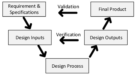
Figure 1.
Design procedure [1,2,3].
The appropriate verification procedure should be chosen depending on the type/nature of the project, the size of the component or the subsystem [4]. Methods of verification using computer simulations are widely used and have become the basis of model-based systems engineering [5]. The development of computer models of a complex system is often cheaper and faster than the construction of real prototypes. Based on computer models and simulations, it is possible to carry out the optimization and verification process. However, also in the case of intensive use of models and computer simulations, measurement verification is needed.
In recent years, there has been a great interest in methods of HIL simulation that combine digital real-time (RT) simulation with actual physical components [6,7]. This is a very useful method for testing expensive and complex physical objects that can be replaced with their computer models. The use of HIL also provides the ability to verify system components under normal and emergency operation conditions [8]. The HIL is widely used in research and industrial laboratories, from problems related to verifying control algorithms, to problems related to mechanical and electrical systems interaction. [6,9,10,11].
Three various types of HIL simulations have been developed for these purposes [10,12,13]:
- Signal-level HIL (SHIL) simulation: the control algorithm and control systems are verified and all other elements are replicated as computer models,
- Power-level HIL (PHIL) simulation: real control and supply systems (power electronics) are verified, the electrical motor and mechanical loads are simulated in RT.
- Mechanical-level HIL simulation (MHIL)—a complete drive system is under test, the mechanical loads (or sources) are emulated using controlled drive system (Figure 2).
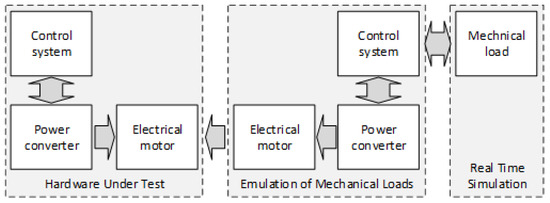 Figure 2. Mechanical-level of Hardware-In-the-Loop (HIL) simulation.
In electric drive technology, the Power-level HIL (PHIL) and Controller-level HIL (CHIL) have been distinguished [14,15,16]. PHIL and CHIL simulations have several profits concerning electric drive validation [17,18,19,20,21,22,23,24,25]. Creating an emulation of the motor, which can be considered as a PHIL simulation, enables the testing of the drive inverter and its control system before the actual motor is developed [26]. The above is accomplished using power amplifiers to emulate motor behaviour [27]. Taking the CHIL into consideration, both the drive inverter and the motor are employed on a real-time simulator. Therefore, both variants of HIL simulation have substantial values regarding rapid prototyping and testing of the electric drive structures.
In the development phase of driving products, the crucial step is the connection with the end-users mechanical systems, when the capabilities of the inverter and the servo-drive are verified. This step is usually time-constricted, as the availability of the customer’s system is often limited. Furthermore, considering large-scale systems, such as cranes, some safety hazards are hard to eliminate from the testing procedures. With existing problems of large machinery and real processes, the use of the HIL approach in the development phase may be crucial [28,29,30,31,32].
The authors [33] propose a model-based development method for industrial machinery drive systems using the HIL simulation system that can integrate various phenomena in mechanical, electrical, and control fields. The proposed method is utilized for the development and verification of a speed control pattern, which does not excite mechanical vibration in a tower crane. The effectiveness of such a method in determining the boundary parameters of a crane drive’s duty cycle is confirmed.
The main focus in the drive design described in this work was the use of high-performance permanent magnet motors for hoist and other crane drives. The use of modern AC drives with permanent magnet motors should provide higher efficiency of the drive system than standard squirrel cage induction motors. At the same time, new propulsion systems should be characterized by high reliability and low noise.
2. Objective and Scope
The main objective of the research is to validate the proposed research methodology. This methodology is developed based on the MHIL concept and incorporates the static and dynamic behaviour of the crane drive systems and the influence of the environmental conditions on the drive’s performance. The validation process is based on the analytical caution, simulations and measurements of the drive systems using a dynamometer test stand controlled by real-time simulations. The scope of the research was established to verify crane drives design assumptions, determine the permissible scope of operation and verify the compliance with the requirements of the EU Machinery Directive [34]. As part of the project titled “Tower crane with permanent magnet electric motors”, research and development were carried out, which included:
- Preparation of simulation models of the electric drive system of the tower crane and simulation of various drive cycles:
- Verification of the correct selection of the structure of the power supply system and control of permanent magnet electric motors,
- Selection of controller parameters in the control system,
- Specifying guidelines for the optimal selection of electric motors and parameterization of the power supply system and machine control.
- Performing experimental tests of the propulsion system components to check and verify that the propulsion system meets the technical assumptions in the field of:
- Lifting speeds for a given weight,
- Movement speeds of the tower crane head for a given weight,
- Power consumption and propulsion efficiency,
- Crane rotation speeds under positive and negative wind loads,
- Determining the level of noise emission in all phases of work,
- Determining the impact of drive operation on the quality of electricity,
- Determining the motor heating curve.
The drives consisting of brushless synchronous motors (AC) with permanent magnets and dedicated inverters were selected for the production of the hoist, jib rotation and trolley travel drive systems. A 16.1 kW motor was selected to drive the hoist winch, a 4.15 kW motor was used to drive the jib rotation and trolley travel. Motor parameters are presented in Table 1.

Table 1.
The parameters of permanent-magnet motors for crane prototype.
The main drive (winches) is implemented using a converter, network filter, braking resistor and a controller. The jib rotation drive and the trolley travel drive is implemented using a permanent magnet motor (servo drive) and a converter. The mechanical characteristics are presented in Figure 3 and Figure 4.
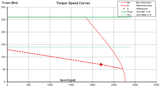
Figure 3.
Mechanical characteristics of the hoist-drive motor with the converter (Udc voltage = 560 V), where: Tpk—curve for S5 duty cycle (intermittent operation with a large number of connections and electric braking), Tc—curve for S1 continuous cycle, Tr—drive operating point, SR_pk—torque limit at maximum current, SR_c—torque limit at rated current.
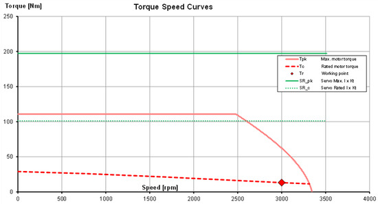
Figure 4.
Mechanical characteristics of the jib rotation and trolley travel drive motor with the converter (Udc voltage = 560 V), where: Tpk—curve for S5 duty cycle (intermittent operation with a large number of connections and electric braking), Tc—curve for S1 continuous cycle, Tr—drive operating point, SR_pk—torque limit at maximum current, SR_c—torque limit at rated current.
The selection of elements of the main electric drive system as well as the jib rotation and trolley travel drives was made based on the motors manufacturer software and the set of the operating conditions (speed, load). As part of the research, simulation calculations were carried out to verify the design assumptions and to analyze the limit performance of the propulsion system. As part of the simulation tests, the following was developed: a program supporting motor selection based on a given motion profile and a simulation model in the MATLAB/SIMULINK environment for the analysis of dynamic states of the propulsion system operation.
Simulations and experimental tests of selected work cycles characteristic of a given drive type were carried out. The tests were carried out in the LINTE^2 Laboratory of the Gdańsk University of Technology on a dynamometer stand, see Figure 5. A special dynamometer control program was developed to emulate the load to which the crane drive systems are subjected. Lifting a load of a given weight, movement of the Jib rotation and trolley travel were simulated in the braking mode. Lowering the weight and weight swing during the work of the crosshead were simulated in the dynamics of the dynamometer. To set the right torque on the shaft of the motor under test, an appropriate dynamometer control algorithm was prepared and a proprietary device for communication with the dynamometer control system and data (speed and torque) acquisition was developed. Communication with the dynamometer controller is done via the Ethernet interface using the Modbus TCP protocol. The torque and speed measured values are read and the set values are saved in each algorithm cycle.
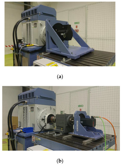
Figure 5.
Permanent magnet motor mounted on the test bench of the dynamometer: (a) for hoist drive, (b) for the drive with the gear of jib rotation and trolley travel.
The main contributions of the proposed research are:
- The proposed research methodology incorporates the MHIL approach, the measurement of electrical, mechanical and thermal parameters of the drive system and the emulation of environmental conditions such as the changes in the ambient temperature.
- The measurements of the limits of the drive system in different conditions such as different drive cycles emulating the real performance of crane drives and the changing supply voltage amplitude representing real construction site conditions.
3. Hoist-Drive System—Simulation Model
The hoist drive consists of the main winch (electric motor, brake, gear, and rope drum) as well as the rope, trolley, hook block, rope wheels and rope attachment point (swivel). The diagram of the main hoist rope is shown in Figure 6. The rope is attached to the hoist drum (a), passing through the cast iron (b) and polyamide (c) wheels on the turntable. Then, the rope is slung over the rope wheels in the hook block and the trolley (d). The end of the rope is attached to the last jib segment (e). The hoist-drive system is equipped with an electromagnetic drum brake to maintain the loads when stopped, but also during an over-speed operation phase.
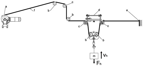
Figure 6.
The diagram of the main hoist rope: (a) the hoist drum, the cast iron (b) and polyamide (c) wheels on the turntable, (d) the trolley, (e) rope attachment point (swivel), (f) rope.
The elements of a drive system (motor, inverter, mains filter, brake resistor and CPU/PLC) were sized based on the expected maximum load and speed analysis. The motor torque (Tm) was calculated based on the equation:
where: is the weight of the hook block and the weight suspended on it, D is the diameter on which the last rope roll is located on the hoist drum (Figure 6a), , are the gear ratio and the efficiency of the pulley block (Figure 6b,c) and , are the gear ratio and the efficiency of the transmission, respectively (Figure 6a).
The rotational speed of the motor was calculated from:
where: vh is the linear lifting speed of the hook.
At the project stage, it was necessary to confirm the validity of the selection of the propulsion system elements. Because the mechanical construction of the crane was not completed and available for testing the verification was carried out in the emulated environment. The crane load characteristics were used to set the speed and torque waveform on the drive motor shaft using a dynamometer.
3.1. Static Simulations
The main purpose of the static simulations was the calculation of the operating points and the selection of the appropriate drive elements based on the crane’s movement profiles.
The movement profile expresses the shape of speed changes during the work cycle and provides a basis for calculating the load torques and selecting the appropriate motor. Several basic shapes of motor speed changes during operation are assumed: trapezoidal, triangular or according to the movement profile with a trapezoidal shape of speed consists of three phases of work: acceleration, work at a constant speed and braking. A special case of the trapezoidal profile is the triangular profile, which eliminates the stage of work at a constant speed—Figure 7. Consequently, the triangular profile consists of only two stages of work: acceleration and braking. As a result, adopting a triangular profile results in higher maximum speeds with smaller accelerations at the same time (Figure 8a). The use of speed changes according to the trapezoidal or triangular profile allows us to easily determine the acceleration and change the position of the displaced load. As a consequence of the trapezoidal or triangular profile of velocity changes, uncontrolled vibrations occur (associated with the lack of limitation of acceleration changes (jerk). Theoretically, the rate of acceleration changes reaches infinitely large values. To reduce vibrations, it is recommended to use the velocity profile described employing s-curves with limitation of acceleration changes (Figure 8b).
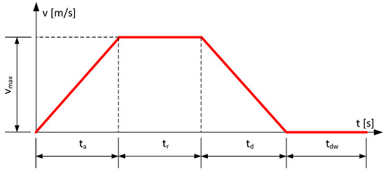
Figure 7.
A trapezoidal velocity profile.
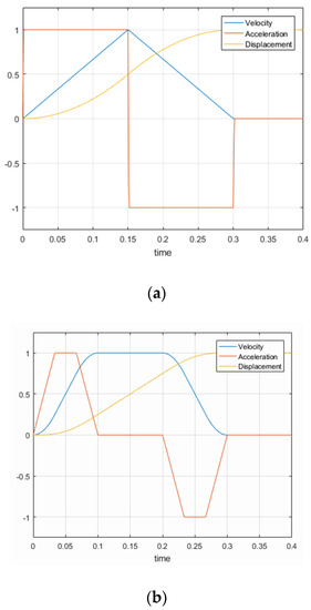
Figure 8.
An example of a traffic profile with (a) a triangular velocity profile, (b) a velocity profile described by s-curves.
The adopted movement profile allows the calculation of the maximum speed value, acceleration of the maximum distance travelled. It was assumed that the total operation time (tm = ta + tr + td) in Figure 7 for:
- (a)
- Trapezoidal profile—acceleration, driving at a constant speed and braking time is indicated in the figure,
- (b)
- Triangular profile—acceleration and deceleration time is 1/2 tm,
- (c)
- The profile described by s-curves—acceleration and deceleration time is the same, each of them is divided into three even stages: acceleration (deceleration) increases linearly, acceleration is constant and acceleration decreases linearly.
The selection of an appropriate speed change profile should take into account the maximum speed limits—resulting from the strength of the mechanical structure (e.g., bearings), limitations of the control system (encoder, controller), available supply voltage and the limits of maximum acceleration—resulting from the strength of the mechanical structure (bearings), peak current. If the criterion is the maximum speed limit, a trapezoidal profile with 1/3 division or an ordinary trapezoidal profile smoothed using s-curves should be used. With such a profile, lower speeds are obtained, but at the same time higher acceleration than with a triangular profile. If the criterion is the limitation of acceleration, the use of a triangular profile or the consideration of extending the time of surgery should be done.
The input data for calculations (Table 2) and the assumed motion trajectory (Table 3) were formulated based on the device catalogue data and project assumptions. The data and trajectory correspond to the work cycle of the main electric drive (winch) of the crane. The preliminary calculation results for checking the correctness of motor selection are presented in Table 4.
Table 2.
Input data for calculations of the motor selection for crane hoist drive.
Table 3.
Trajectory parameters of the lifting movement.
Table 4.
Checking calculation results for the correctness of hoist motor selection.
When sizing the motor, select the motor whose maximum speed is greater than the calculated maximum speed and the maximum torque is greater than the calculated maximum torque value and which will provide the appropriate effective torque value. The obtained calculation results placed in points 29, 30, 34, 35 and 36 of Table 4 confirm the correctness of choosing the drive.
As a result of the software calculations, information is obtained regarding exceeding the permissible motor values (speed, torque, current, power). The calculated operating points of the drive are compared with the limit characteristics of the motor (and converter) on the graph of the torque dependence on the motor speed (Figure 9). When choosing the motor and converter, it is necessary to choose devices that will provide appropriate values for maximum current, effective current, electrical power and voltage at the terminals. Exceeding the maximum voltage values at the motor terminals and DC bus is permissible when switching to the appropriate motor control ensuring torque limit and de-excitation (reduction of the resultant excitation field in the machine).
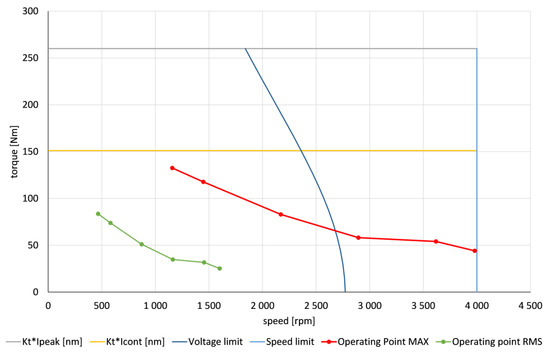
Figure 9.
The results of calculations of the motor selection program for the main tower crane drive along with the drive limiting characteristics.
Similarly, calculations were carried out by static simulation for the selection of the motor for a jib rotation drive and a trolley travel drive system.
3.2. Dynamic Simulations
A simplified simulation model was prepared in the commercial MATLAB program. Such dynamic simulation was used for calculations of winding temperature for a given duty cycle. The model is based on analytical dependencies taking into account the basic elements of the propulsion system (converter, motor, mechanical transmission, weight) and energy dependencies.
The following describes the process of heating the electric motor as a result of current flow in the armature winding. The temperature rise was defined as:
where: is the winding temperature and is the ambient temperature.
The thermal behaviour is determined by the equation:
where: is the winding specific heat, is the winding mass, is the thermal resistance,
where are copper losses.
The solution is:
The product of thermal resistance [C/W], specific heat [J/kg/K] and mass has a time dimension and the thermal time constant is determined:
Assuming an initial condition such that the initial temperature is equal to the ambient temperature:
one obtains:
or when taking into account the initial temperature difference or the temperature from the previous step:
For discrete-time values and small increments dt, one can use approximation:
For a given motion profile, the courses of speed and linear acceleration of weight, displacement, resultant force, rotational speed, the angular acceleration of the motor, motor shaft torque, electric power, motor current and voltage at the terminals are determined (Figure 10a–f). The simulation program prepared can be used to estimate the temperature of the motor windings at a given duty cycle (Figure 10g).
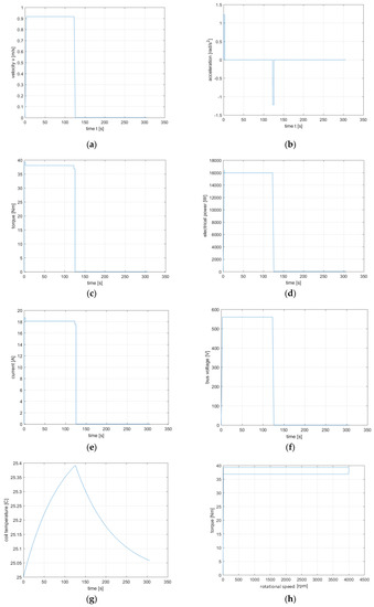
Figure 10.
The work cycle of the main electric drive of the tower crane: (a) velocity waveform, (b) acceleration waveform, (c) torque waveform, (d) electrical power waveform, (e) current waveform, (f) bus-voltage waveform, (g) motor coil temperature, (h) mechanical characteristic.
Maintaining the set operating temperature below the permissible temperature is possible with proper selection of the duty cycle. In the case of operation with a load greater than the rated (permissible permanently), appropriate break time between cycles must be ensured. The maximum speed in the work cycle should be lower than the maximum mechanical speed specified in the catalogue. Operating the motor at a speed greater than the rated speed requires adequate motor control to reduce the excitation flux and limit the voltage on the DC bus. As a consequence, a reactive component appears in the motor supply current, the purpose of which is to reduce the excitation flux from permanent magnets. The additional current component requires a reduction of the active motor component and, consequently, lower active power and torque on the shaft. This functionality is built into the control and power supply system of the motor.
Similarly, calculations were carried out by dynamic simulation for the selection of the motor for a jib rotation drive and a trolley travel drive system.
4. Mechanical-Level Hardware-In-The-Loop Testing for Drives
4.1. Hoist (Main) Drive
The main element of the Mechanical-level HIL (MHIL) system was the dynamometer of electrical machines. In combination with additional control and data acquisition systems, this is a useful device for testing and verifying prototypes in emulated operating conditions. The tested permanent magnet motors were mounted on the test bench and coupled to the dynamometer shaft. The additional control system was used to emulate crane load characteristics (speed and torque acting on the motor shaft). For this purpose, a master controller based on the Raspberry Pi microcomputer was developed.
Communication between the master controller and the dynamometer controller was done using the Ethernet interface and the Modbus TCP protocol. The simplified structure of the measurement system is shown in Figure 11. A graphical interface for controlling the program was developed, which allows setting the dynamometer work parameters (Figure 12).
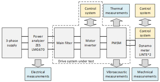
Figure 11.
The simplified structure of the measurement system.
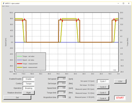
Figure 12.
A graphical interface for the control software used to emulate crane load characteristics.
The emulation of the tower crane operation is carried out by the set of the torque waveform corresponding to the load of the drive motor when lifting and lowering the weight. The tests were run in a loop. The control algorithm takes into account the operation of the mechanical brake (Figure 13).
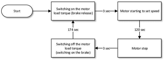
Figure 13.
The dynamometer control algorithm emulating the activation of the mechanical brake after motor stopping.
After stopping the drive motor, the load torque is removed from the shaft with a three-second delay, simulating the engagement of the brake. After the set time has expired and in 3 s before motor engaging the brake is released. At this point, the load torque is again applied to the drive motor shaft. After the reset time of 3 s, the motor restarts and works with the set load torque which corresponds to lifting or lowering the set weight.
During the drive’s testing, the motor housing temperature and the winding temperature were recorded. To record the temperature of the motor housing, a thermal imaging camera and temperature sensors were glued to the housing. The results of temperature measurements from the camera were archived in photographic, film and text files with the temperature of the selected place on the motor housing (Figure 14a). The pyrometer was also used to control the external temperature. The winding resistance of the tested machines was measured:
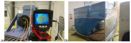
Figure 14.
Registration of the motor housing temperature during the test (a) and a view of the dynamometer stand adapted to obtain an elevated ambient temperature (b).
- A.
- Directly on the main drive motor using a winding temperature sensor—the signal from the temperature sensor was recorded using the converter control software;
- B.
- Indirectly, in the case of the other 2 motors, the winding temperature is based on changes in the winding resistance during the motor warm-up attempt.
For the indirect method of temperature measurement, a system that would with predetermined time intervals stop the on-load measurements of the drive system and automatically switch to resistance measurement before switching back to the on-load operation was used. A greenhouse foil dynamometer stand cover was prepared for tests at elevated ambient temperature (Figure 14b). The ambient temperature of T = 40 °C was obtained with external heaters.
A work cycle was developed to emulate raising and lowering a given weight at a given speed. The control system of the dynamometer set the required torque on the motor shaft: braking torque during the lifting and the driving torque during lowering (Figure 15). The velocity of lifting and lowering of the weight was controlled by the motor control system (Figure 16a). The results of mechanical measurements are presented per unit, related to the speed and torque set values.
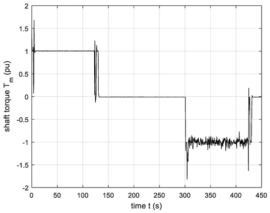
Figure 15.
The torque measured on the motor shaft during emulation of the work cycle consisting of lifting and lowering the constant weight, defined in the per-unit system (p.u.).
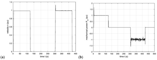
Figure 16.
The velocity (a) and mechanical power (b) measured on the motor shaft during emulation of the work cycle consisting of lifting and lowering the constant weight, defined in per-unit system (p.u.).
Oscillations in the torque waveform (Figure 15) result from the control method of the drive. Dynamic changes in acceleration and associated with this jerk value in combination with dynamometer stand inertia are causing dynamic changes in measured torque. The test bench regulator can set the required torque after 0.2 s. However, if the measured speed at any point during the test reaches a negative value in reference to the set direction of motion, the dynamometer test stand is disabled. This can happen when the drive is decelerating and stopping, the inertia of the drive and the test stand can cause the speed to reach negative values. When this occurs the dynamometer is disabled, the control algorithm detects this and re-enables the dynamometer after 0.5 s.
The mechanical power (Figure 16b) is calculated as the product of the rotational speed and torque measured by the dynamometer. The positive value of torque and mechanical power means the work of the crane when lifting the weight, negative values correspond to lowering the weight.
The measurement of electrical quantities was carried out using the ZES LMG670 power analyzer. Among other things, the RMS values of voltage and current supplying the inverter and the electrical power delivered to the inverter (Figure 17) were recorded. The results of electrical measurements are presented per unit. During braking, the power was dissipated in the braking resistor and not returned to the grid thus the inverter input current is not flowing during the dynamic braking stage when lowering the weight.
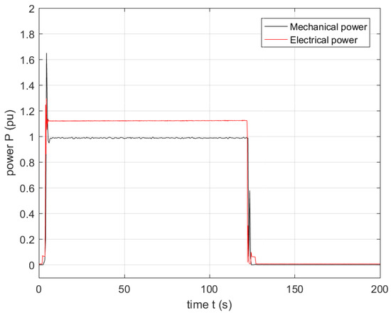
Figure 17.
Electrical power delivered to the motor inverter vs. mechanical power on the motor shaft – lifting the weight, defined in the per-unit system (p.u.).
The efficiency of the prototype crane drive system, which was 88%, was determined from the ratio of mechanical power on the motor shaft and the electric power supplied to the inverter (Figure 17).
Furthermore, tests were carried out on the impact of reduced supply voltage on the winch drive system operation. The converter supply voltage was reduced at a given constant motor load. Two motor-load levels were set:
- A.
- The operation with maximum weight: torque T = 130 Nm, set speed n = 1500 rpm—20.4 kW active power,
- B.
- The operation without additional weight: torque T = 10 Nm, set speed n = 3780 rpm—active power approximately 4 kW.
The outcomes of those tests are presented in Figure 18. At the first load level A, the drive operated at a set speed across the entire voltage range (280–400 V). In the case of the second load level B, the drive operated at a set speed at a voltage above 380 V. A drop in supply voltage below 380 V caused a decrease in motor speed. At 290 V, the motor speed dropped to 2830 rpm, with active power limited to 3 kW. This only shows the drive performance and its limit regarding the deexcited operation.
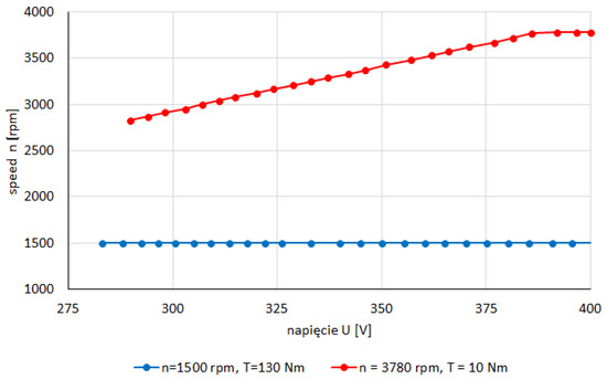
Figure 18.
Winch drive operation at a reduced supply voltage.
This performance at a reduced supply voltage can be quantified using measurement data and expressed as:
where U is the supply line-to-line voltage and n is the rotational speed of the drive.
4.2. Trolley Travel Drive
The permanent-magnet motor with the converter selected for the trolley travel drive in MHIL was also tested on the dynamometer. Experimental studies were performed using a dynamometer test stand designed for lower power electric machines. Appropriate software to control the dynamometer was developed to map the work cycle of the trolley travel drive. For each of the given work cycles, an analysis of the test results was carried out to determine:
- Power consumption and efficiency of the propulsion system,
- Determining the level of noise emissions in all operating phases,
- Determining the impact of drive operation on the quality of electricity.
It was assumed that the longest path that the crosshead can cover is 60 m. Experimental studies were carried out for the following cycles:
- A.
- The maximum speed of 60 m/min, driving for 1 min 30 s break, motor speed 3070 rpm, resistance torque 3.5 Nm;
- B.
- The maximum speed of 45 m/min, driving 1 min 20 s, 30 s break, motor speed 2300 rpm, resistance torque 4.3 Nm;
- C.
- The maximum speed of 30 m/min, driving 2 min, 30 s break, motor speed 1540 rpm, resistance torque 9.2 Nm.
An important feature of the crosshead’s work is the need to accelerate and slow down a heavy load (inertia), which may tend to rock. The impact of uncontrolled weight swings was modelled by setting the appropriate torque. During the acceleration and deceleration phase, a sinusoidal variable with an amplitude of 2.5 × Tust was added, as shown in Figure 19.
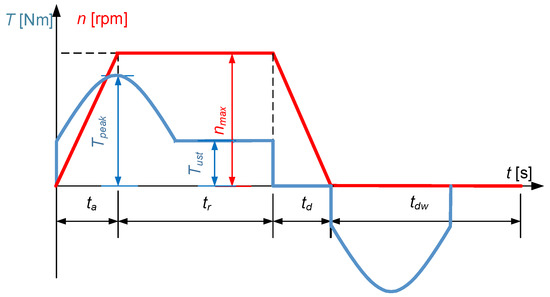
Figure 19.
The set course of changes in the set speed and the resistance moment of the trolley travel drive.
The waveforms of speed, mechanical moment and mechanical power recorded for cycle C on the shaft of the tested motor are, for example, shown in Figure 20.
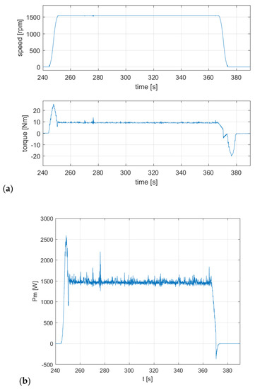
Figure 20.
Recorded waveforms of torque, speed (a) and mechanical power (b) on the motor shaft during a given cycle of work C.
A summary of mechanical and electrical measurements of the average results during operation at a constant speed for A and C cycle is given in Table 5. Table 5 also contains the effective results of recorded values supplying the drive unit’s converter. Repeated analogous measurements for cycle B showed a reduction in power unit efficiency to 66%. This resulted from increased mechanical losses by higher speeds.
Table 5.
Measurement results for C and A cycle of the trolley travel drive.
The waveforms of speed and mechanical moment and mechanical power recorded for A cycle on the shaft of the tested motor are, shown in Figure 21. The efficiency of the electric drive system working in cycle A is 75.5% (Table 5). Despite the greater mechanical losses (higher rotational speed), the drive works by consuming less current and, therefore, less active losses in the windings. As a result, the efficiency in this cycle is less than in cycle C but greater than in cycle B.
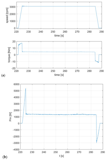
Figure 21.
Recorded waveforms of torque, speed (a) and mechanical power (b) on the motor shaft during a given cycle of work A.
4.3. Jib Rotation Drive
The permanent-magnet motor with the converter selected for the jib rotation drive was also tested using the MHIL approach and the dynamometer test bench. Experimental studies were performed using a dynamometer for lower power electric machines. Appropriate software to control the dynamometer was developed to map the work cycle of the turntable drive. For each of the given work cycles, an analysis of the test results was carried out to determine:
- Power consumption and efficiency of the propulsion system,
- Determining the level of noise emissions in all operating phases,
- Determining the impact of drive operation on the quality of electricity.
Experimental studies were carried out for the following cycle: trapezoidal speed waveform in which the rise time, constant speed 1560 rpm, constant torque 37 Nm and braking time are the same and amount to 15s. The set stopping time is the 30 s. The braking moment is applied during acceleration and deceleration and taken off while driving at a constant speed (Figure 22).
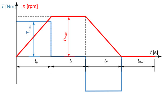
Figure 22.
The profile of changes in the set speed and the torque of the jib rotation drive.
The waveforms of speed, mechanical moment and mechanical power recorded on the shaft of the tested motor are shown in Figure 23. A summary of mechanical and electrical measurements of the average results during operation at the cycle is given in Table 6. Table 6 also contains the effective results of recorded supplying values the drive unit’s converter. The results showed the power unit efficiency of 88%.
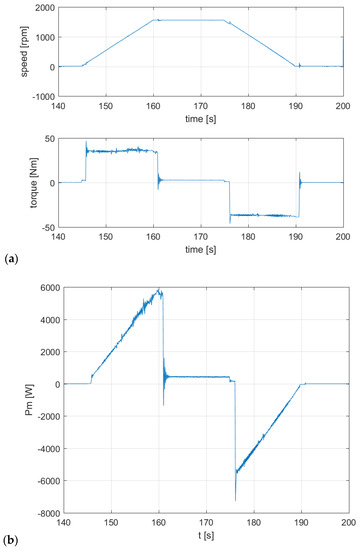
Figure 23.
Jib rotation drive’s operating cycle: (a) set courses of rotational speed, (b) loading moment and calculated mechanical power.
Table 6.
Measurement results for the cycle of the jib rotation drive.
5. Preliminary Conclusions Regarding the Efficiency of the Tested Drives
The obtained efficiency results do not allow for a direct assessment of the drives proposed for the tower crane prototype in terms of compliance with standards. Degrees and efficiency classes (“IE”) of electric motors are defined in the IEC 60034-30-1: 2014 standard. The standard applies to single-speed electric motors powered by a sinusoidal voltage source. The classification includes motors with rated power from 0.12 kW to 1 MW, rated voltage from 50 V to 1 kV, with 2, 4, 6 or 8 poles, designed for continuous operation at rated load and at a temperature rise below that permissible with due to the insulation class, in the ambient temperature range from −20 °C to +60 °C and at an altitude of up to 4 km above sea level.
The aforementioned standard does not apply to the tested motors as they are 5-pole motors designed for intermittent operation and powered from a converter. Assessment of the efficiency class of the tested motors determined by comparing the efficiency determined based on experimental tests with the minimum value of the efficiency of machines with 8 poles and 15 kW and 18.5 kW, frequency 50 Hz, according to IEC 60034-30-1: 2014.
However, based on the developed charts (Figure 24a) it can be stated concerning the main drive that the efficiency of the tested motor for loads below the rated torque (Tn = 70 Nm) is on average 91% (at maximum, 94%) which corresponds to class IE3 (premium efficiency) or IE4 (super premium efficiency) for this machine power.
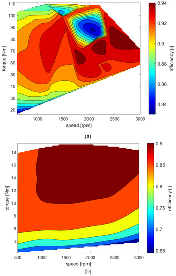
Figure 24.
Efficiency points of the main motor of the crane drive (a) and the trolley travel and jib rotation drive (b) on the torque characteristics as a function of speed.
Concerning the other two crane drives, based on the developed charts Figure 24b it can also be stated that the efficiency of the tested motors for loads above 6 A and 14 Nm exceeds 85% reaching a maximum value of about 86%, which corresponds to class IE3 (premium efficiency) or IE4 (super premium efficiency) for this power machines.
6. Conclusions
The experimental tests of selected operating cycles of prototype crane drives were carried out. Experimental research was performed in the LINTE^2 laboratory, where a mechanical level of the HIL simulator was developed. The most important device of the system was the dynamometer with the control system. A special program to control the dynamometer and to emulate the load for which the crane was developed. A series of tests related to electric motor environmental parameters was carried out.
As a result of the tests, it was shown that the prototype crane drive system meets both the requirements specified in the project assumptions and concerning the relevant standards. The use of high-performance permanent magnet motors allowed for the entire drive efficiency of 88%.
The methodology described in the above work allows for a verification of the drive system of large-scale machinery utilizing a large-capacity motor without using actual power inverters, motors, and associated machines so that even software or a control engineer can adapt it easily. Such a laboratory test-bed is essential when restrictions in the power source environment, installation location, or safety aspects prohibit on-site testing. Moreover, the effect of the communication period and communications delay between instruments on control performance can be evaluated also for use with high accuracy such as synchronous control. Therefore, using the described method for the verification of a drive system of industrial machinery allows one to discover, in advance, the possible complications linked to real system examination and to take actions against them during future development.
Author Contributions
Conceptualization, M.M. and F.K.; methodology, M.M. and F.K.; software, F.K. and Ł.S.; validation, D.K., R.R. and Ł.S.; formal analysis, R.R., Ł.S., G.K.; investigation, D.K.; resources, R.R., Ł.S.; data curation, R.R.; writing—original draft preparation, M.M., F.K., R.R., D.K.; writing—review and editing, M.M., D.K., R.R., Ł.S.; visualization, G.K., B.G.; supervision, D.K., B.G.; project administration, M.M. All authors have read and agreed to the published version of the manuscript.
Funding
The research has been carried out under a contract with a special-purpose company of the Gdańsk University of Technology EXCENTO for the benefit of Krupiński Cranes Sp. z o.o., dealing with the design and production of tower cranes. Financial resources for the research service come from the Intelligent Development Operational Program 2014–2020, Sub-measure 1.1.1 Industrial research and development works carried out by enterprises.
Conflicts of Interest
The authors declare no conflict of interest.
References
- Butler, M.; Petre, L.; Sere, K. (Eds.) Model Driven Engineering, volume 2335/2002 of Lecture Notes in Computer Science; Springer: Berlin/Heidelberg, Germany, 2002; Volume 2335. [Google Scholar]
- Skjetne, R.; Egeland, O. Hardware-in-the-loop testing of marine control system. Model. Identif. Control. 2006, 27, 239–258. [Google Scholar] [CrossRef]
- Contreras-Moreno, G.; Toledo, G. (Preliminary Concept) Design of a Mechatronic System to Relief Search and Rescue of Victims after an Earthquake Disaster. Ph.D. Thesis, Fachhochschule Aachen, Aachen, Germany, 2018. [Google Scholar]
- ISO. 9001 Design Verification and Validation—EBS Quality, EBS Quality Solutions, 18 June 2018. Available online: https://www.ebsindy.com/iso-9001-design-verification-and-validation/ (accessed on 10 April 2019).
- NASA. Systems Engineering Handbook; NASA: Washington, DC, USA, 2019.
- Faruque, M.D.O.; Strasser, T.; Lauss, G.; Jalili-Marandi, V.; Forsyth, P.; Dufour, C.; Dinavahi, V.; Monti, A.; Kotsampopoulos, P.; Martinez, J.A.; et al. Real-Time Simulation Technologies for Power Systems Design, Testing, and Analysis. IEEE Power Energy Technol. Syst. J. 2015, 2, 63–73. [Google Scholar] [CrossRef]
- Morawiec, M.; Blecharz, K.; Lewicki, A. Sensorless Rotor Position Estimation of Doubly Fed Induction Generator Based on Backstepping Technique. IEEE Trans. Ind. Electron. 2020, 67, 5889–5899. [Google Scholar] [CrossRef]
- Ogan, R.T. Hardware-In-The-Loop Simulation; Springer: London, UK, 2015. [Google Scholar]
- Lauss, G.F.; Faruque, M.O.; Schoder, K.; Dufour, C.; Viehweider, A.; Langston, J. Characteristics and Design of Power Hardware-in-the-Loop Simulations for Electrical Power Systems. IEEE Trans. Ind. Electron. 2016, 63, 406–417. [Google Scholar] [CrossRef]
- Carmeli, M.S.; Castelli-Dezza, F.; Mauri, M.; Marchegiani, G. A Novel Mechanical Hardware in the Loop Platform for Distributed Generation Systems. Distrib. Gener. Altern. Energy J. 2013, 28, 7–27. [Google Scholar] [CrossRef]
- Leisten, C.; Jassmann, U.; Balshüsemann, J.; Hakenberg, M.; Abel, D. Design and Analysis of a MPC-based Mechanical Hardware-in-the-Loop System for Full-Scale Wind Turbine System Test Benches. IFAC-Pap. 2017, 50, 10985–10991. [Google Scholar] [CrossRef]
- Facchinetti, A.; Mauri, M. Hardware-in-the-Loop Overhead Line Emulator for Active Pantograph Testing. IEEE Trans. Ind. Electron. 2009, 56, 4071–4078. [Google Scholar] [CrossRef]
- Bouscayrol, A. Different Types of Hardware-In-the-Loop Simulation for Electric Drives. In IEEE International Symposium on Industrial Electronics; IEEE: New York, NY, USA, 2008; pp. 2146–2151. [Google Scholar]
- Amitkumar, K.S.; Pillay, P.; Belanger, J. Hardware-in-the-loop Simulations of Inverter Faults in an Electric Drive System. In Proceedings of the 2019 IEEE Energy Conversion Congress and Exposition (ECCE), Baltimore, MD, USA, 29 September–3 October 2019. [Google Scholar]
- Pellegrino, L.; Sandroni, C.; Bionda, E.; Pala, D.; Lagos, D.T.; Hatziargyriou, N.; Akroud, N. Remote Laboratory Testing Demonstration. Energies 2020, 13, 2283. [Google Scholar] [CrossRef]
- Ebe, F.; Idlbi, B.; Stakic, D.E.; Chen, S.; Kondzialka, C.; Casel, M.; Heilscher, G.; Seitl, C.; Bründlinger, R.; Strasser, T.I. Comparison of Power Hardware-in-the-Loop Approaches for the Testing of Smart Grid Controls. Energies 2018, 11, 3381. [Google Scholar] [CrossRef]
- Amitkumar, K.S.; Kaarthik, R.S.; Pillay, P. A versatile power-hardware-in-the-loop-based emulator for rapid testing of transportation electric drives. IEEE Trans. Transp. Electrif. 2018, 4, 901–911. [Google Scholar] [CrossRef]
- Kennel, R.M.; Boller, T.; Holtz, J. Replacement of Electrical (Load) Drives by a Hardware-in-the-Loop System. In Proceedings of the International Aegean Conference on Electrical Machines and Power Electronics and Electro-Motion Joint Conference, Istanbul, Turkey, 8–10 September 2011; pp. 17–25. [Google Scholar]
- Vodyakho, O.; Steurer, M.; Edrington, C.S.; Fleming, F. An induction machine emulator for high-power applications utilizing advanced simulation tools with graphical user interfaces. IEEE Trans. Energy Convers. 2012, 27, 160–172. [Google Scholar] [CrossRef]
- Masadeh, M.A.; Amitkumar, K.S.; Pillay, P. Power electronic converter-based induction motor emulator including main and leakage flux saturation. IEEE Trans. Transp. Electrif. 2018, 4, 483–493. [Google Scholar] [CrossRef]
- Saito, K.; Akagi, H. A power hardware-in-the-loop (P-HIL) test bench using two modular multilevel DSCC converters for a synchronous motor drive. IEEE Trans. Ind. Appl. 2018, 54, 4563–4573. [Google Scholar] [CrossRef]
- Schmitt, A.; Richter, J.; Gommeringer, M.; Wersal, T.; Braun, M. A Novel 100 kW Power Hardware-in-the-Loop Emulation Test Bench for Permanent Magnet Synchronous Machines with Nonlinear Magnetics. In Proceedings of the 8th International Conference on Power Electronics Machines and Drives (PEMD 2016), Glasgow, UK, 19–21 April 2018; pp. 1–6. [Google Scholar]
- Sutő, Z.; Balogh, A.; Kiss, D.; Veréb, S.; Varjasi, I. Power Hil Emulation of AC Machines with Parallel Connected ANPC Bridge Arms. In Proceedings of the IEEE 18th International Power Electronics and Motion Control Conference (PEMC), Budapest, Hungary, 26–30 August 2018; pp. 592–598. [Google Scholar]
- Morawiec, M.; Lewicki, A. Application of Sliding Switching Functions in Backstepping Based Speed Observer of Induction Machine. IEEE Trans. Ind. Electron. 2020, 67, 5843–5853. [Google Scholar] [CrossRef]
- Lee, Y.; Kwon, Y.; Sul, S. DC-link Voltage Design of High-Bandwidth Motor Emulator for Interior Permanent-Magnet Synchronous Motors. In Proceedings of the IEEE Energy Conversion Congress and Exposition (ECCE), Portland, OR, USA, 23–27 September 2018; pp. 4453–4459. [Google Scholar]
- Drobnič, K.; Gašparin, L.; Fišer, R. Fast and Accurate Model of Interior Permanent-Magnet Machine for Dynamic Characterization. Energies 2019, 12, 783. [Google Scholar] [CrossRef]
- Blecharz, K.; Morawiec, M. Nonlinear Control of a Doubly Fed Generator Supplied by a Current Source Inverter. Energies 2019, 12, 2235. [Google Scholar] [CrossRef]
- Zhuang, X.; Hibino, S.; Harakawa, M.; Terabe, R.; Ozaki, T.; Nagano, T. Hardware-In-the-Loop Simulation of a Machine Model with Real-Time Animation. In Proceedings of the 2014 International Power Electronics Conference (IPEC-Hiroshima 2014—ECCE ASIA), Hiroshima, Japan, 18–21 May 2014; pp. 2638–2643. [Google Scholar]
- Jarzebowicz, L. Errors of a Linear Current Approximation in High-Speed PMSM Drives. IEEE Trans. Power Electron. 2017, 32, 8254–8257. [Google Scholar] [CrossRef]
- Wachowiak, D. Genetic Algorithm Approach for Gains Selection of Induction Machine Extended Speed Observer. Energies 2020, 13, 4632. [Google Scholar] [CrossRef]
- Dworakowski, P.; Wilk, A.; Michna, M.; Fouineau, A.; Guillet, M. Lagrangian model of an isolated dc-dc converter with a 3-phase medium frequency transformer accounting magnetic cross saturation. IEEE Trans. Power Deliv. 2020, 35, 10. [Google Scholar] [CrossRef]
- Kutt, F.; Michna, M.; Kostro, G. Multiple Reference Frame Theory in the Synchronous Generator Model Considering Harmonic Distortions Caused by Nonuniform Pole Shoe Saturation. IEEE Trans. Energy Convers. 2020, 35, 166–173. [Google Scholar] [CrossRef]
- Nagano, T.; Harakawa, M.; Ishikawa, J.; Iwase, M.; Koizumi, H. Model Based Development Using Hardware-in-the-Loop Simulation for Drive System in Industrial Machine. Mech. Eng. Robot. Res. 2019, 8, 46–51. [Google Scholar] [CrossRef]
- OJEU. Directive 2006/42/EC of the European Parliament and of the Council of 17 May 2006 on Machinery, and Amending Directive 95/16/EC; OJEU: Aberdeen, UK, 17 May 2006. [Google Scholar]


Publisher’s Note: MDPI stays neutral with regard to jurisdictional claims in published maps and institutional affiliations. |
© 2020 by the authors. Licensee MDPI, Basel, Switzerland. This article is an open access article distributed under the terms and conditions of the Creative Commons Attribution (CC BY) license (http://creativecommons.org/licenses/by/4.0/).