Article

Voltage Stability Analysis in Medium-Voltage Distribution Networks Using a Second-Order Cone Approximation

by
Oscar Danilo Montoya
1,2,
Walter Gil-González
3,
Andrés Arias-Londoño
3,
Arul Rajagopalan
4 and
Jesus C. Hernández
5,*
1
Facultad de Ingeniería, Universidad Distrital Francisco José de Caldas, Bogotá D.C 11021, Colombia
2
Laboratorio Inteligente de Energía, Universidad Tecnológica de Bolívar, Cartagena 131001, Colombia
3
Facultad de Ingeniería, Institución Universitaria Pascual Bravo, Campus Robledo, Medellín 050036, Colombia
4
School of Electrical Engineering, Vellore Institute of Technology, Chennai 632014, India
5
Department of Electrical Engineering, Campus Lagunillas s/n, University of Jaén, Edificio A3, 23071 Jaén, Spain
*
Author to whom correspondence should be addressed.
Energies 2020, 13(21), 5717; https://doi.org/10.3390/en13215717
Submission received: 28 August 2020 / Revised: 8 October 2020 / Accepted: 23 October 2020 / Published: 2 November 2020
(This article belongs to the Special Issue Voltage Stability Analysis in Power Systems)

Abstract

:
This paper addresses the voltage stability margin calculation in medium-voltage distribution networks in the context of exact mathematical modeling. This margin calculation is performed with a second-order cone (SOCP) reformulation of the classical nonlinear non-convex optimal power flow problems. The main idea around the SOCP approximation is to guarantee the global optimal solution via convex optimization, considering as the objective function the λ -coefficient associated with the maximum possible increment of the load consumption at all the nodes. Different simulation cases are considered in one test feeder, described as follows: (i) the distribution network without penetration of distributed generation; (ii) the distribution network with penetration of distributed generation; and (iii) the distribution grid with capacitive compensation. Numerical results in the test system demonstrated the effectiveness of the proposed SOCP approximation to determine the λ -coefficient. In addition, the proposed approximation is compared with nonlinear tools available in the literature. All the simulations are carried out in the MATLAB software with the CVX package and the Gurobi solver.

1. Introduction

Electrical distribution networks are a sub-component of the power system required for interconnecting end-users with the transmission and sub-transmission systems at the substation points [1]. They can cover thousands of kilometers in medium-voltage levels to provide electricity service to urban and rural areas [2,3]. Due to their extensions, they have higher power losses compared with the transmission system [4]. Furthermore, electrical distribution networks may also be more sensitive to voltage instabilities since they are typically operated in a radial structure [5,6]. In the scientific literature, the voltage stability problems in distribution networks are usually addressed via indices based on the voltage profile and load consumption. The authors in [7] studied the problem of voltage stability in AC distribution networks with large-scale photovoltaic generation developing a voltage stability index as a function of the line parameters, power demands, and voltages calculated with a classical power flow approach. They demonstrated via numerical simulations that depending on the renewable energy penetration on a particular node, the voltage stability index can be improved or worsened presenting guidelines for optimal location of these devices. In [8], a voltage stability index was proposed to identify the nodes close to the verge of voltage collapse. Its proposed voltage stability index value was calculated at each node of the distribution grid using a modified load flow method for voltage stability analysis. The modified load flow method incorporated composite load modeling and variations in load patterns at each node. Additionally, the results in [8] were found satisfactory compared with the other known methods of voltage sensitivity indices. The authors in [9] presented the classical Newton-Raphson method’s extension based on the continuation point for voltage stability analysis in distribution networks. Their numerical results showed the efficiency in the 33-nodes test feeder with low-computational effort. Their results were also compared with specialized tools such as PSAT for MATLAB, reaching a minor error when the λ -coefficient is calculated. In [10], an uncertainty quantification approach for phasor measurement units (PMUs) in voltage stability evaluation was described. In [11], the calculation of a voltage stability margin in radial distribution system was presented considering a unique reactive loading index. In [12], a static voltage stability index in AC distribution systems was proposed using the network-load admittance ratio. This index showed a behavior highly linear with a load increase. In [13], a theoretical voltage stability analysis for AC distribution networks was presented. This analysis determined some essential practical points such as static power reserve until the voltage instability phenomenon, static voltage stability limit, and maximum active power. In [14], the impact on voltage stability margin in an islanded microgrid was studied considering photovoltaic generation. It is worth mentioning that in the the case of DC distribution networks, some approaches in relation with determining voltage stability margin have been reported in literature. In [15] the authors have proposed a semidefinite programming model calculation of the voltage stability margin in DC grids with constant power loads considering a monopolar grid connection. Numerical results demonstrated that the SDP approach reaches the global optimum comparing its results with multiple nonlinear solvers available in the general algebraic modeling system (GAMS). The authors of [16] have presented the problem of the λ -coefficient calculation in DC grids using interior point methods available in GAMS in a tutorial style. In reference [17] it has been proposed an approach to calculate the voltage stability index in DC networks by using the determinant of the Jacobian matrix as a function of load increments controlled by a linear function. Numerical results have demonstrated the possibility of reaching the global optimum when compared with nonlinear programming and semidefinite programming approaches. The main advantage lies mainly in its easy implementation at any programming language.
After the revision of the state-of-the-art, we identify a gap in the literature regarding the voltage stability analysis, which is related to the existence of convex mathematical formulation for voltage stability analysis in AC distribution networks in the optimization context. The convex analysis is a part of the exact mathematical optimization that exploits the structure of solution spaces and objective functions to solve complex problems that guarantee the global optimum [18]. For the voltage stability analysis, a second-order cone programming (SOCP) formulation of the nonlinear modified optimal power flow problem in the complex domain is proposed to compute the voltage stability margin ( λ -coefficient) in distribution networks. Numerical results in the 33-nodes test feeder demonstrate that the proposed SOCP model reaches the global optimum of the problem compared with multiple nonlinear solvers available in the (GAMS) [16]. The proposed approach from convex optimization results comfortable to implement at any programming language and avoids the classical usage of the continuation method that requires an adequate parameterization to guarantee convergence.
This paper is organized as follows: Section 2 presents the exact nonlinear formulation of the voltage stability margin calculation using a modified version of the optimal power flow problem. Section 3 presents the SOCP formulation to calculate the λ -coefficient in distribution systems, highlighting the main advantage that consists of finding the optimum global. Section 4 provides the main characteristic of the 33-nodes test feeder and the simulation cases. Section 5 presents all the numerical simulations, analysis and discussion. Section 6 gives the main concluding remarks derived from this research and some guidelines for future avenues of research.

2. Exact Formulation

The problem of the voltage stability margin calculation in distribution networks can be represented with a nonlinear programming model, considering as the objective function the analysis of the λ coefficient [19]. This parameter allows to know the maximum simultaneous increment at all the loads before voltage-collapse [20]. The main complicated constraints of this model corresponds to the power balance equations, which are nonlinear due to the hyperbolic relation between voltages and powers at each node. The mathematical formulation of this problem is presented below.

2.1. Objective Function

The objective function of this problem corresponds to the loadability coefficient of the whole distribution grid, which is maximized and can be written mathematically, as follows
min z = λ ,
where z is the objective function value, and λ represents the maximum chargeability coefficient.

2.2. Set of Constraints

The set of constraints associated with the problem of the voltage stability margin calculation are described below.
S i c g + S i d s 1 + λ S i d = V i i = 1 n Y i j V j , i N
where V i C is the voltage value at node i; S i c g C is the apparent power generation at node i by the conventional generator, i.e., the slack node; S i d s C is the apparent power generation at node i by a distributed source, i.e., distributed generators or capacitor banks; S i d C is the apparent power consumption at node i; Y i j C corresponds to the component of the admittance matrix Y C n × n that relates nodes i and j. Note that N is the set that contains all the nodes which has a cardinality equal to n; and () is the complex conjugate operator.
V i 1 γ , i N
where γ is a real positive constant that is related to the maximum deviation of the voltage profile at each node when the load increases constantly. For simulation purposes, it can be defined between 0.4 and 0.8 [9].
Due to the nature of the λ -coefficient the following constraint is added to the optimization model
λ 0 .
The interpretation of the NLP model (1)–(4) is presented below: Equation (1) corresponds to the objective function of the voltage stability problem in distribution networks which deals with computing the maximum loadability factor of the grid. This allows for understanding the margin of stable operation regarding load increments and possible expansion projects. The constraint (2) corresponds to the set of power balance equations regarding apparent power equilibrium based on the second Tellegen’s theorem. Expression (3) corresponds to the voltage regulation constraint, which is relaxed to determine the maximum loadability factor of the grid. Finally, Expression (4) presents the positiveness definition of the λ -coefficient.
Remark 1.
The problem of voltage stability margin calculation in distribution networks is a nonlinear non-convex optimization problem due to Expression (2) that shows the hyperbolic relation between voltage and power at each node, which generates a set of non-affine quadratic constraints. To solve this problem, the power flow equations can be treated with a second-order cone equivalent model that transforms the exact NLP model defined from (1) to (4) into a SOCP equivalent convex reformulation.

3. SOCP Reformulation

The second-order cone programming approach is a branch of the convex optimization that allows to transform a type of nonlinear programming problems using conic constraints (i.e., representation using norms), that warranties the global optimum solution of the problem due to its convex structure [21,22]. In the case of the power flow problem, in the literature it has been demonstrated that SOCP approximations allow to have the zero-duality gap between the exact NLP model and its conic transformation [23]. Here we present the SOCP transformation of the voltage stability margin calculation model (1)–(4), which allows the global optimal solution, which is not possible with heuristic approaches. Note that the SOCP transformation of this model only requires to rewrite the product between voltage variables in (2) by using a new variable as presented below:
W i j = V i V j ,
with the new variable W i j , the power balance Equation (2) takes the following form:
S i c g + S i d s 1 + λ S i d = i = 1 n Y i j W i j . i N
Remark 2.
The power balance constraint defined in (6) is now at a set of an affine set of constraints in the complex domain, which implies that it is convex.
To guarantee that the new variable W i j allows recovering the original voltage variables V i , an additional set of constraints is incorporated as described below.
Let us pre-multiply both side of Expression (5) by W i j , which produces:
W i j W i j = V i V j V i V j W i j 2 = V i V j .
Now, based on the definition (5) we can use an auxiliary variable as W i i = V i , which implies that Equation (7) can be redefined as
W i j 2 = W i i W j j .
Note that the right-hand-side of (8) can be represented using its hyperbolic representation as follows:
W i i W j j = 1 4 W i i + W j j 2 1 4 W i i W j j 2 ,
which implies that if we substitute (10) in (8), then, we reach the following result
W i j 2 + 1 4 W i i W j j 2 = 1 4 W i i + W j j 2 .
Observe that Expression (10) can be shown using norms as presented below:
2 W i j W i i W j j = W i i + W j j .
Remark 3.
Expression (11) is still non-convex due to the equality structure; however, in power systems as demonstrated in [18], this can be relaxed by changing the equality symbol into the lower equal symbol as follows
2 W i j W i i W j j W i i + W j j ,
where now it is a conic convex constraint.
To complete the SOCP representation of the voltage stability margin calculation, we rewrite (3) in its standard form as
1 γ V i 1 + γ , i N
that can be rewritten by using W i i as follows
1 γ 2 W i i 1 + γ 2 . i N
Note that (14) is a box-type constraint which is convex.
Remark 4.
The SOCP approximation for the exact NLP model (1)–(4) proposed in this research is defined by the set of Equations (1), (4), (6) and (12). The main advantage of the proposed SOCP model is the opportunity to guarantee the global optimum due to the convex structure of the solution space [18].

4. Test Systems and Simulation Scenarios

To validate the effectiveness and robustness of the proposed SOCP programming model to determine the voltage stability margin in AC medium voltage distribution test feeders with global optimum capabilities, we employ two classical AC medium-voltage networks composed of 33 and 69 nodes, respectively. The information of these test feeders and the simulation cases is presented below.

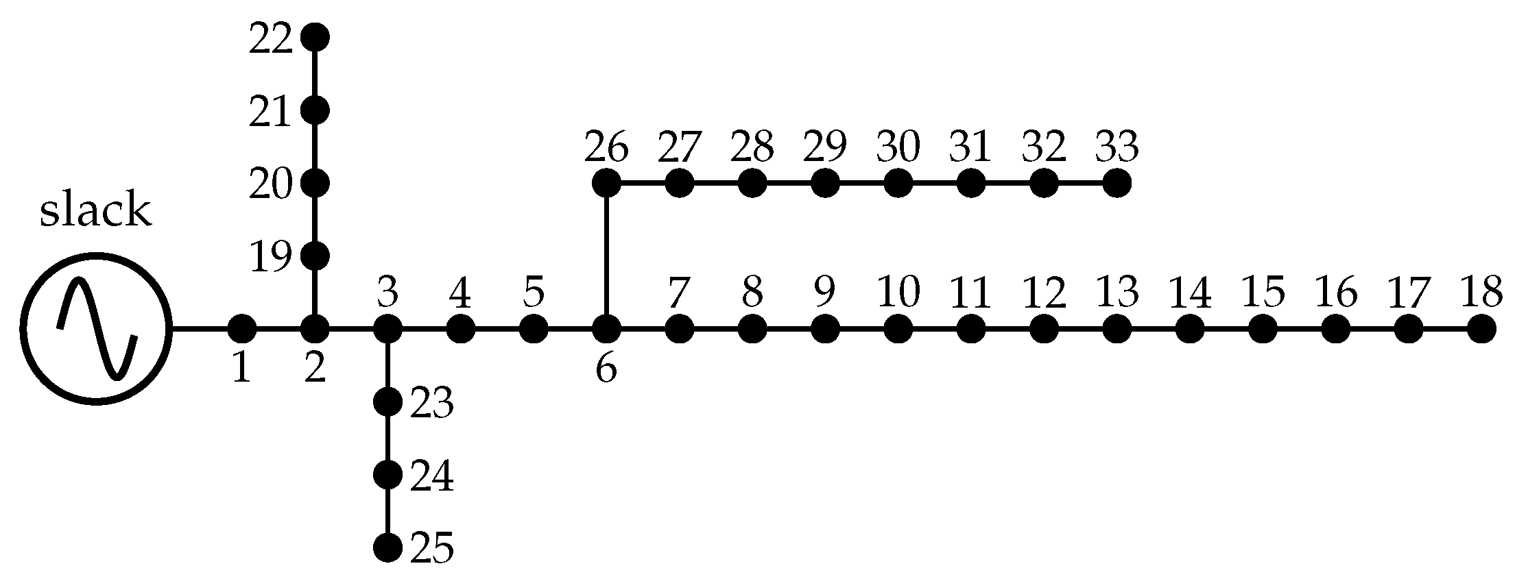
4.1. 33-Nodes Test Feeder

The validation of the proposed SOCP model is made in a classical radial distribution test feeder composed of 33-nodes and 32 lines operated at a nominal voltage of 12.66 kV. The grid configuration of this test feeder is depicted in Figure 1, and its branches and load information are reported in Table 1.
In this feeder, the total active power demand is 3715 kW and total reactive power demand is 2300 kVAr. For simulation purposes, we consider 100 kVA and 12.66 kV as power and voltage base respectively.

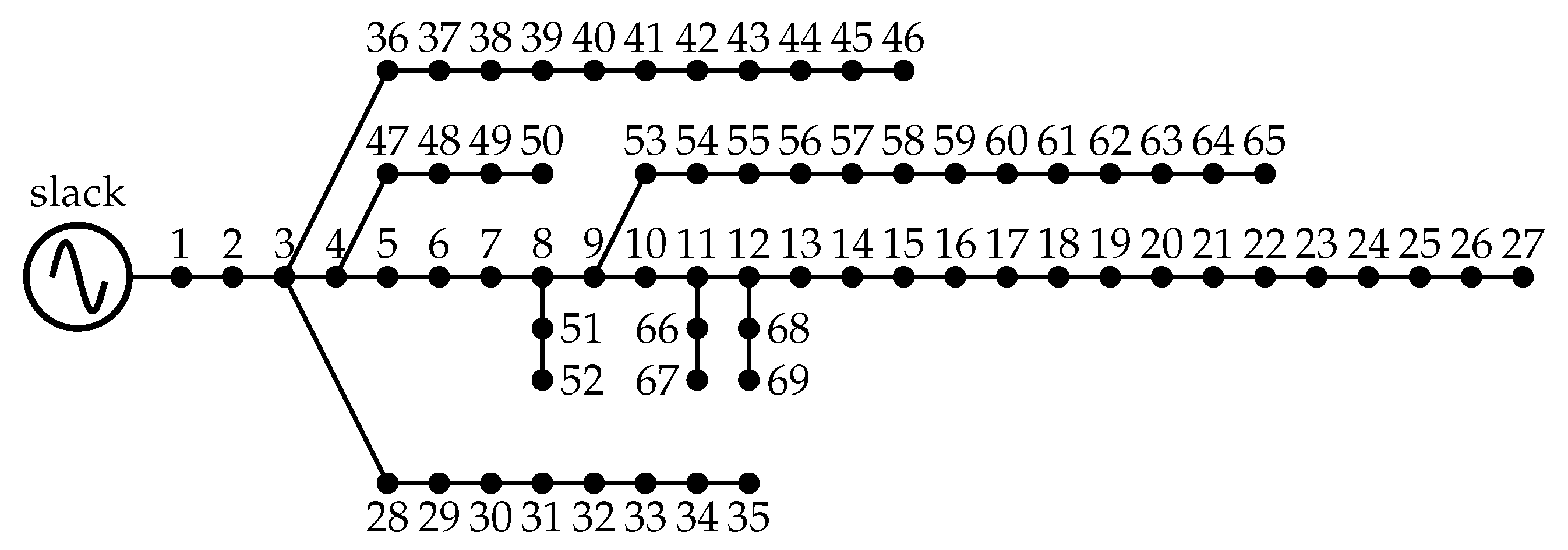
4.2. 69-Nodes Test Feeder

The 69-nodes test feeder is widely known in the literature as the Baran & Wu test feeder which is composed of 69 nodes and 68 branches, and operated at the voltage controlled node with 12.66 kV. The electrical configuration of this test feeder is reported in Figure 2 and all the parametric information regarding nodes and branches are presented in Table 2.
In this feeder the total active power is 3890.7 kW and the total reactive power is 2693.6 kVAr. For simulation purposes, we consider 100 kVA and 12.66 kV as power and voltage base respectively.

4.3. Simulation Scenarios

The validation of the proposed voltage stability margin calculation in AC distribution networks is performed in this research based on the following simulation cases.
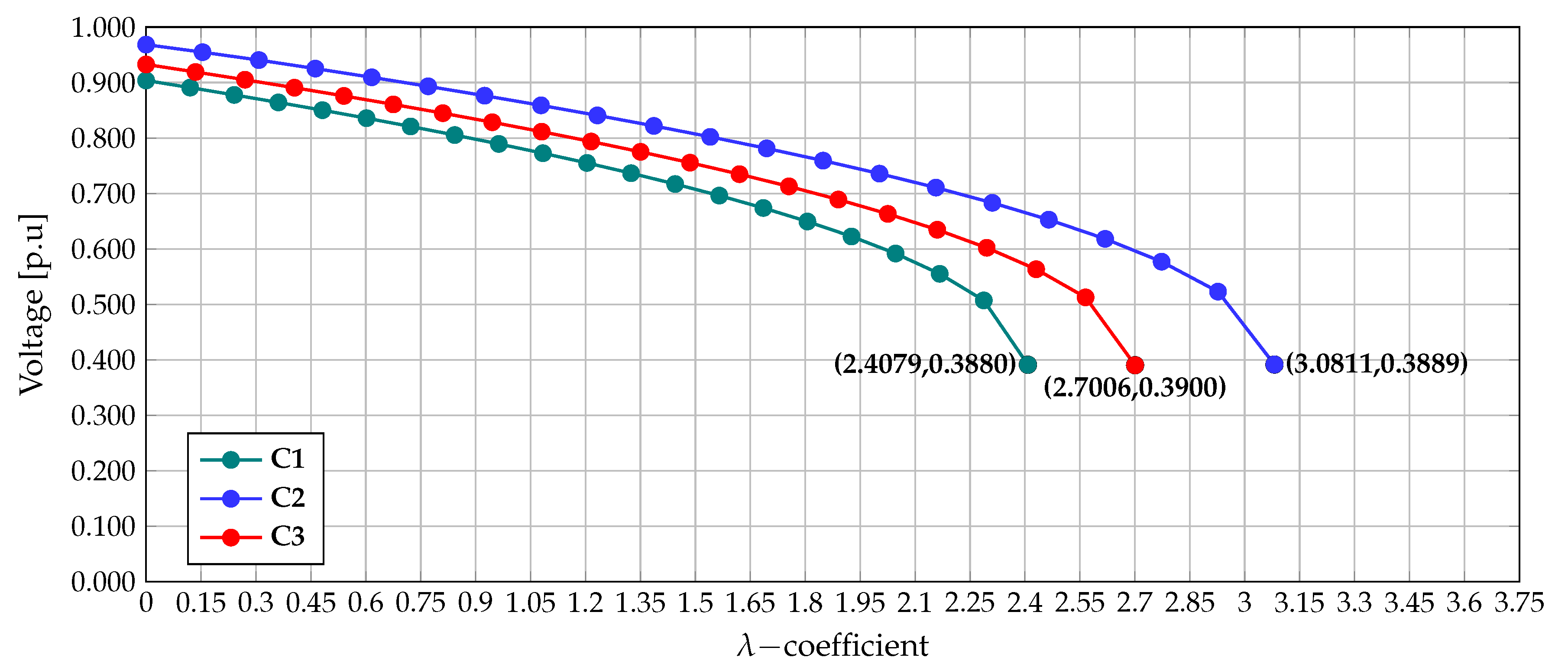
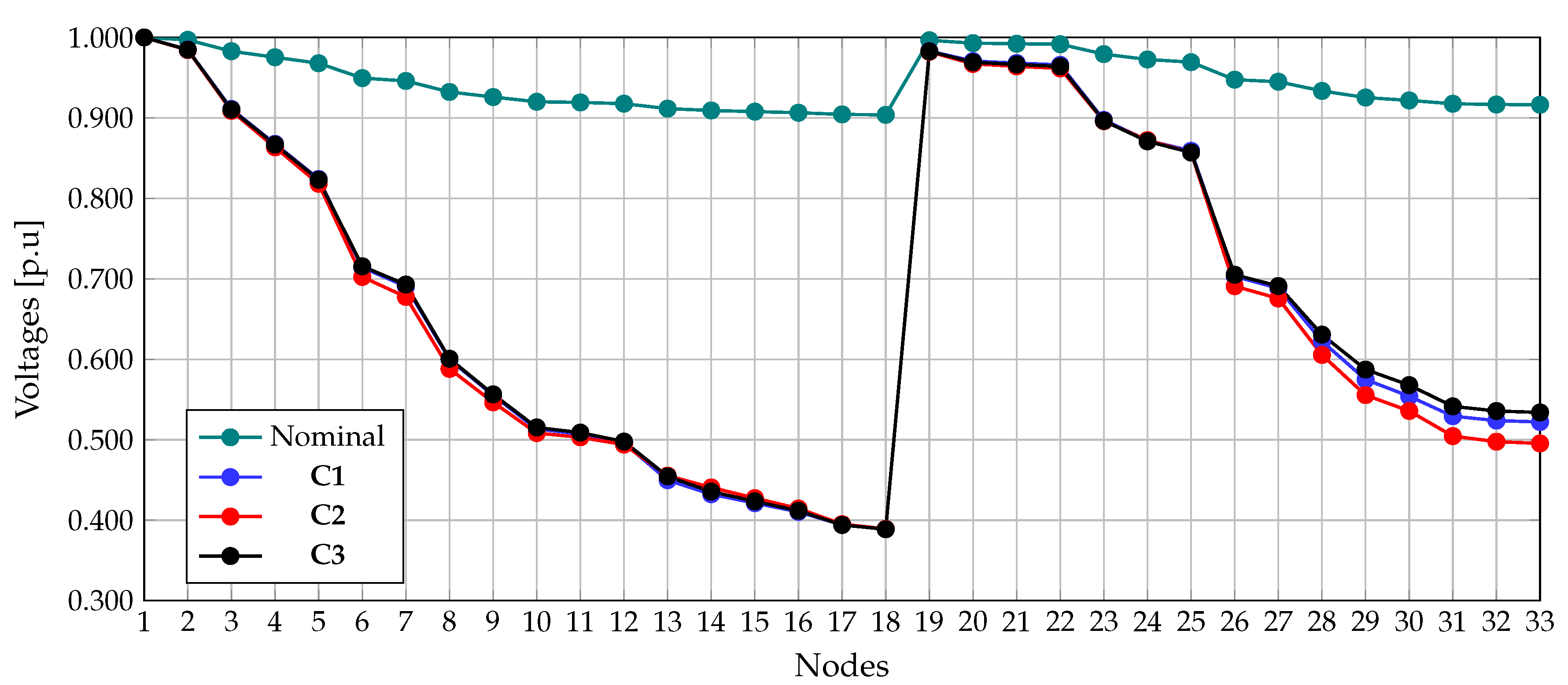
Case 1 (C1): The original configuration of the AC distribution network; i.e., without penetration of distributed generation or capacitor banks.
Case 2 (C2): The operation of the distribution network considering the location of distributed generators reported in [24] which are operated with unity power factor.
Case 3 (C3): The operation of the distribution network considering the location of fixed-step capacitor banks as recommended in [25].
For simulation cases 2 and 3, we consider the following distributed generators and fixed step capacitor banks:
For the 33-nodes test feeder in the C2 the distributed generators are included at nodes 14, 24, and 30 with power injections of about 770.9 kW, 1096.9 kW and 1065.8 kW, respectively. On the other hand, for capacitor banks in the C3, we consider two banks of 450 kVAr located at nodes 13 and 24, and a bank of 900 kVAr positioned at node 30.
For the 69-nodes test feeder in the C2, the distributed generators are included at nodes 12, 61, and 64 with power injections of about 813.1 kW, 1444.7 kW and 289.6 kW, respectively. For capacitor banks in the C3, we consider two banks of 300 kVAr located at nodes 11 and 18, and a bank of 1200 kVAr positioned at node 61.

5. Computational Validation

Implementing the SOCP approximation for voltage stability margin determination in distribution networks is carried out with the CVX tool using the MOSEK solver by using the MATLAB software version 2019b in on a desktop computer with an INTEL(R) Core(TM) i 7 7700 2.8-GHz processor and 16.0 GB of RAM running on a 64-bit version of Microsoft Windows 10 Home.

5.1. 33-Nodes Test Feeder

For this test feeder we consider two simulation conditions, the first one corresponds to the three cases simulation case, and the second one is associated to the effect that the renewables have in the loadability factor including daily load variations.

5.2. Evaluation of the Simulation Cases

In this simulation scenario it is considered the original formulation proposed in Equations (1), (4), (6) and (12) to determine the voltage stability margin for all the nodes considering all the simulation cases. Note that to verify that the solution provided by the SOCP model is optimal, we implement the exact nonlinear model (1)–(4) in the GAMS software with different NLP solvers. Table 3 presents the λ -coefficient for each simulation case.
Results in Table 3 demonstrate that the proposed SOCP model finds the global optimum solution of the voltage stability margin determination in the case of the 33-nodes test feeder. Additionally, we can observe that: (i) the injection of active power by distributed generation (see C2) allows to increment the voltage stability margin about 27.92% respect to the base case (i.e., C1); and (ii) the injection of reactive power also allows to increase the voltage stability margin about 12.11%; however, its impact is lower when compared with the active power case. This behavior is explained since the total injection of active power is about 2933.6 kW, while the reactive power is 1800 kVAr.
Remark 5.
The solution of the voltage stability margin in the 33-nodes test feeder via convex and nonlinear optimization methods reported in Table 3, neglecting their small differences, is the same reported by the continuation method reported in [9], which confirms the efficiency of our convex approximation in comparison with classical methods [7].
Figure 3 presents the voltage performance at all the nodes of the 33-nodes test feeder for the nominal case, considering all the simulation cases.
Note that throughout all the loadability cases, the minimum voltage at point of collapse is presented at node 18 with a magnitude of 0.3888 pu. However, we can observe that C2 allows lower voltage profiles in the case of nodes upper than 26. This behavior is expected since the load increments in this scenario are larger than C1 and C3, as presented in Table 3.
Figure 4 presents the voltage behavior of the node 18 since, as depicted in Figure 3. This is the node that reaches the minimum voltage value at each simulation case.
Figure 4 confirms that the injection of the active and reactive power in some nodes of the distribution network increases the voltage stability margin in all the nodes of the network, as demonstrated in [26]. This implies that the problem of the optimal location of capacitor banks and/or distributed generators is a subject currently under study, since these devices have substantial impacts regarding voltage stability, power losses, and voltage regulation improvements [27].
Remark 6.
The proposed SOCP approximation has allowed us to determine the maximum chargeability coefficient for the 33-nodes test feeder in different operation cases, guaranteeing its global optimal solution. In addition, numerical results demonstrate that the voltage collapse point is far from the nominal operation case for the 33-nodes test feeder. This means that to reach the instability point over all the loads, these must be increased at least 2.4 times, which in practice will not occur since the protection system will operate much before of this case. However, the proposed SOCP is general, useful to identify instability scenarios even if these are very closely to the nominal operation case.
Regarding processing times, we can mention that all the NLP solvers in GAMs and the proposed SOCP approach take less than 10 ms to find the solution of the voltage stability margin problem, which implies that from the computational effort perspective, we can confirm that all the methodologies are efficient; however, in terms of solution quality, the best methodology is the SOCP approach.

5.3. Effect of Renewables in the Stability Margin

To present the effect of the renewable energy penetration in the voltage stability index for distribution networks, consider the 33-nodes test feeder as recommended in [28,29] with the penetration of photovoltaic and wind turbine sources. The connection of the generators for each test system is presented as follows: at node 13, it is connected a photovoltaic generator PV1 and a wind turbine WT1 with nominal rates of 450 kW and 825 kW, respectively. At node 25, it is connected a second photovoltaic source PV2 with a nominal power rate of 1500 kW while at node 30, it is connected the second wind power source named WT2 with a rate capability of 1200 kW. The hourly behavior of these generators is reported in Table 4.
In the case of the demand power’s daily behavior, the load curve reported in [30] is considered as depicted in Figure 5.
Figure 6 presents the behavior of the voltage stability margin in the 33-nodes test feeder considering different levels of power generation penetration, which is defined from 0 to 100% of the power generation reported in Table 6 in steps of 25%.
From Figure 6, we can observe that:
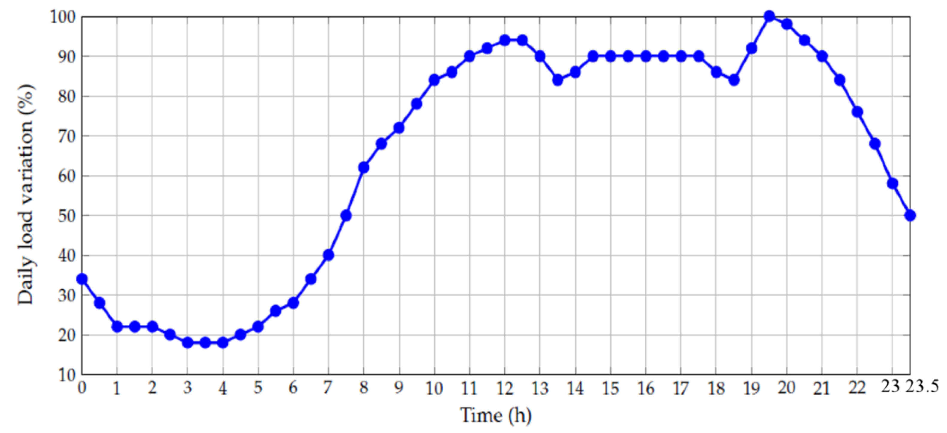
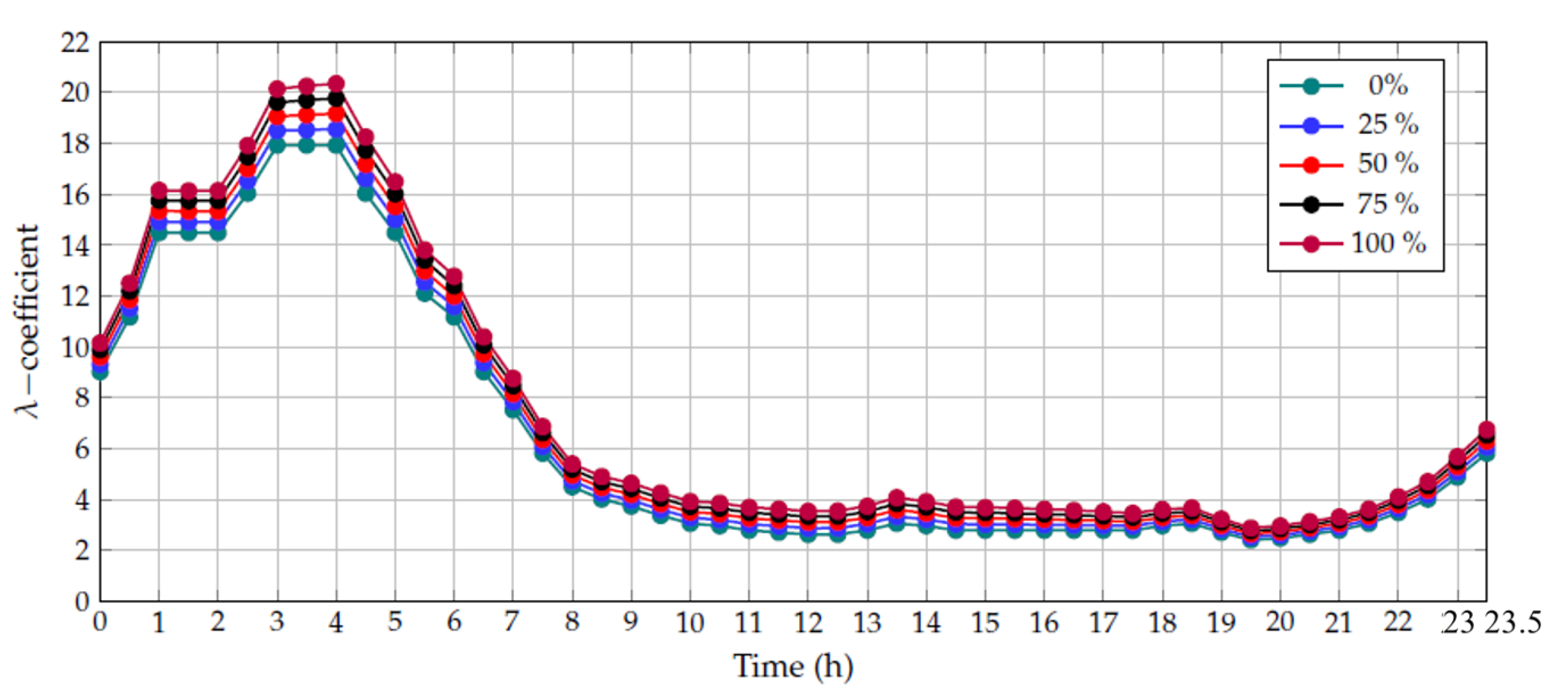
In the time periods when the demand is low (see the period between 0 h and 8 h in Figure 5), the λ -coefficient is higher taking values upper than 6 with a maximum between 18 and 22 in the period between 3 and 5 h. This behavior is explained by the fact that the chargeability coefficient is a factor that multiplies the load at each operating condition. This implies that for low demands, this will increase until the point of the voltage-collapse.
For the time periods with higher demand (upper than 10 h in Figure 5) it is possible to see that the λ -coefficient oscillates between 2 and 4, and we also observe that depending on the level of distributed generation penetration, this increases respect to the base case (0% of renewable generation availability), i.e., the renewable generation has positive effects regarding voltage stability margin since for all the penetration cases the loadability coefficient is enlarged.
Note that the minimum λ -coefficient is presented at 19.5 h. At this point when the renewable energy penetration is 0%, the λ -coefficient is 2.407 (see Table 3 for the C1), and when the renewable energy penetration is 100%, this factor is 2.883. Note that this modest increment is because the renewable generation based on photovoltaic is zero at this time and the wind power is also in low values; nevertheless, this increment contributes to the voltage stability margin improvement.

5.4. 69-Nodes Test Feeder

In this section it is computed the voltage stability margin for the 69-nodes test feeder considering all simulation cases 1 to 3. Table 5 presents the numerical results reached by the proposed SOCP and the NLP solvers available in the GAMS optimization package.
Numerical results in Table 5 confirms that the proposed SOCP reformulation can deal with the global optimum of the studied optimization problem which matches with the solutions reported by the GAMS solvers. Additionally, the numerical performance of the cases C2 and C3 show that the injection of the active and reactive power allows enlarging the voltage stability margin in 32.84% and 12.03% respectively. These are expected results, since these local injections reduce the total consumption observed in the distribution network, which is directly connected to the rate of power increments allowed on them and measured by the λ -coefficient.
Regarding processing times as reported for the 33-nodes test feeder, the proposed SOCP reformulation and the GAMS solvers take less than 10 ms to find the optimal solution of the problem. This low-computational effort shows the efficiency of all the studied methods to solve the voltage stability margin in radial distribution networks with considerable number of nodes, i.e., 33 and 69, respectively.
When the voltage profiles are analyzed in the 69-nodes test feeder, in the case C1 the minimum voltage is experienced at node 65 with 0.4700 pu; in addition, for the cases C2 and C3 the minimum values result at the same node (i.e., node 65) with magnitudes of 0.4740 pu and 0.4660 pu respectively. The interpretation of these values is as follows: (i) these correspond to the maximum voltage drop on the distribution network under extreme load conditions; however, these values will never occur under real operation, since protection schemes regarding low-voltages will disconnect the distribution network to protect all the components; and (ii) the λ -coefficients reported in Table 5 can be understood as grid efficiency indicators, since the farther from zero they are, the more robust the distribution network is unser load increments, due to that the λ -coefficient measures the extreme load condition where the distribution grid will present a voltage collapse.

5.5. Additional Results

The proposed SOCP model corresponds to an adequate optimization methodology to deal with finding the global optimum, ensuring convergence with low-computational effort. Even if the GAMS package can deal with the global optimum there are two main problems when using it for large-scale nonlinear optimization as follows: (i) it is not possible to ensure mathematically the global optimum due to the non-convexities of the solution space given by the power balance equations, and (ii) it requires a commercial license to deal problems with thousands of variables, while the proposed SOCP model is suitable for being implemented in free software such as Phyton with available tools for solving convex optimization problems [31].
In addition, here, we present a possible application where the usage of the SOCP allows to reach the global optimum of mixed-integer programming problems which is not possible with mixed-integer NLP models solvable in the GAMS software. For doing so, consider that in the 33-nodes test feeder it is possible to locate three distributed generators with capabilities of generation from 0 kW to 1200 kW considering a penetration equivalent to 60% of the total demand under normal operative conditions. Table 6 presents the solution of the optimal sizing and location of distributed generators in AC distribution networks, to improve the voltage stability margin with different GAMS solvers as well as using a branch MI-SOCP solver via branch & bound methods [32].
Once the numerical results reported in Table 6 are obtained, we can mention that:
All the MINLP solvers available in GAMS, different optimal solutions are reached, which oscillate between 3.3010 and 3.3184. In addition, these solvers identify different nodes and sizes of the distributed generators being node 32 the most recurrent location in all the solutions.
The MI-SOCP strategy allows finding the global optimal solution of this problem with a λ -coefficient of 3.3187. We can ensure that this is indeed the global optimum since an exhaustive search has been implemented to evaluate all the possible combinations. After 2 h of simulations, the combination of nodes 15, 18, and 32 is the best possible scheme to enlarge the voltage stability margin in the 33-nodes test feeder.
Regarding processing times it is worth mentioning that the GAMS solvers and the proposed MI-SOCP have faster performance to obtain optimal solutions since running time of all the simulation cases was lower than 10 s. This is considered in literature a negligible time in planning purposes, since physical installations of these distributed generators can take several weeks or months.
The most important fact from the results reported in Table 6 is that the optimization approach that uses the SOCP formulation to solve the continuous optimization part of the optimal location of distributed generators in distribution networks, allow to find the global optimum, if the branch & bound method is combined with it as demonstrated in [33]. This result confirms the importance of using convex optimization tools when possible in distribution network analysis.

6. Conclusions and Future Works

The problem of determining the voltage stability margin in AC distribution networks has been addressed in this paper under the context of the exact mathematical optimization, proposing a second-order cone programming reformulation for the exact nonlinear model. Numerical validations in the 33- and 69-nodes test feeders have demonstrated that the proposed SOCP approach converges to the global optimum compared with different NLP solvers available in the GAMS optimization package. The injection of active and reactive power in some nodes allowed to demonstrate that the λ -coefficient increases respect to the base case, which implies that these power injections had positive effects on the network’s voltage stability margin. The 24-h operative scenario confirmed these results with renewable power source and load variation. Depending on the percentage of renewable, the loadability coefficient always increase respect to the base case.
The hybridization of the proposed focus of SOCP with a branch & bound approach demonstrates the efficiency of using convex optimization in complex optimization problems that involves binary variables, since it (i.e., MI-SOCP) has demonstrated global optimization capabilities, that are not possible with MINLP solvers available in GAMS. These latter have stuck in local optimal solutions due to the non-convexities of the continuous optimization part of the problem. This result confirms the effectiveness and robustness of using convex optimization in AC distribution analysis when possible.
For future work, it will be possible to perform: (i) extend the proposed SOCP programming formulation to an MI-SOCP (mixed-integer-SOCP) to optimal locating and sizing distributed generators and capacitor banks for voltage stability improvement in AC distribution networks; (ii) apply the proposed analysis to the case of the operation of distribution networks with battery energy storage systems; and (iii) make a comparison between voltage stability indexes reported in the literature and the proposed SOCP model to identify if this voltage stability analysis is compatible.

Author Contributions

Conceptualization, O.D.M., W.G.-G., and J.C.H.; Methodology, O.D.M. and W.G.-G.; Investigation, O.D.M. and W.G.-G.; Writing—review and editing, O.D.M., W.G.-G., A.A.-L., A.R. and J.C.H. All authors have read and agreed to the published version of the manuscript.

Funding

This research was funded by the Agencia Estatal de Investigación, Spain (AEI) and the Fondo Europeo de Desarrollo Regional (FEDER) aimed at the Challenges of Society (Grant No. ENE 2017-83860-R “Nuevos servicios de red para microredes renovables inteligentes. Contribución a la generación distribuida residencial”).

Acknowledgments

This work was partially supported by the National Scholarship Program Doctorates of the Administrative Department of Science, Technology, and Innovation of Colombia (COLCIENCIAS), by calling contest 727-2015.

Conflicts of Interest

The authors declare no conflict of interest.

References

  1. Temiz, A.; Almalki, A.M.; Kahraman, Ö.; Alshahrani, S.S.; Sönmez, E.B.; Almutairi, S.S.; Nadar, A.; Smiai, M.S.; Alabduljabbar, A.A. Investigation of MV Distribution Networks with High-Penetration Distributed PVs: Study for an Urban Area. Energy Procedia 2017, 141, 517–524. [Google Scholar] [CrossRef]
  2. Hernández, J.; Medina, A.; Jurado, F. Impact comparison of PV system integration into rural and urban feeders. Energy Convers. Manag. 2008, 49, 1747–1765. [Google Scholar] [CrossRef]
  3. Montoya, O.D.; Gil-González, W.; Giral, D.A. On the Matricial Formulation of Iterative Sweep Power Flow for Radial and Meshed Distribution Networks with Guarantee of Convergence. Appl. Sci. 2020, 10, 5802. [Google Scholar] [CrossRef]
  4. Jiménez, R.; Serebrisky, T.; Mercado, J. Sizing Electricity Losses in Transmission and Distribution Systems in Latin America and the Caribbean; Techreport; Inter-American Development Bank: Washington, DC, USA, 2014. [Google Scholar]
  5. Prakash, K.; Lallu, A.; Islam, F.; Mamun, K. Review of Power System Distribution Network Architecture. In Proceedings of the 2016 3rd Asia-Pacific World Congress on Computer Science and Engineering (APWC on CSE), Nadi, Fiji, 5–6 December 2016; IEEE: Piscataway, NJ, USA, 2016. [Google Scholar] [CrossRef]
  6. Zaheb, H.; Danish, M.S.S.; Senjyu, T.; Ahmadi, M.; Nazari, A.M.; Wali, M.; Khosravy, M.; Mandal, P. A Contemporary Novel Classification of Voltage Stability Indices. Appl. Sci. 2020, 10, 1639. [Google Scholar] [CrossRef] [Green Version]
  7. Ghaffarianfar, M.; Hajizadeh, A. Voltage Stability of Low-Voltage Distribution Grid with High Penetration of Photovoltaic Power Units. Energies 2018, 11, 1960. [Google Scholar] [CrossRef] [Green Version]
  8. Ranjan, R.; Das, D. Voltage Stability Analysis of Radial Distribution Networks. Electr. Power Compon. Syst. 2003, 31, 501–511. [Google Scholar] [CrossRef]
  9. Aly, M.M.; Abdel-Akher, M. A continuation power-flow for distribution systems voltage stability analysis. 2012 IEEE International Conference on Power and Energy (PECon), Kota Kinabalu, Malaysia, 2–5 December 2012; IEEE: Piscataway, NJ, USA, 2012. [CrossRef]
  10. Chen, C.; Wang, J.; Li, Z.; Sun, H.; Wang, Z. PMU uncertainty quantification in voltage stability analysis. IEEE Trans. Power Syst. 2014, 30, 2196–2197. [Google Scholar] [CrossRef]
  11. Sumit, B.; Chattopadhyay, T.K.; Chanda, C.K. Voltage stability margin of distribution networks for composite loads. In Proceedings of the 2012 IEEE Annual IEEE India Conference (INDICON), Kochi, India, 7–9 December 2012; IEEE: Piscataway, NJ, USA, 2012; pp. 582–587. [Google Scholar] [CrossRef]
  12. Song, Y.; Hill, D.J.; Liu, T. Static voltage stability analysis of distribution systems based on network-load admittance ratio. IEEE Trans. Power Syst. 2018, 34, 2270–2280. [Google Scholar] [CrossRef]
  13. Triştiu, I.; Iantoc, A.; Poştovei, D.; Bulac, C.; Arhip, M. Theoretical analysis of voltage instability conditions in distribution networks. In Proceedings of the 2019 IEEE 54th International Universities Power Engineering Conference (UPEC), Bucharest, Romania, 3–6 September 2019; IEEE: Piscataway, NJ, USA, 2019; pp. 1–5. [Google Scholar] [CrossRef]
  14. Sinder, R.L.; Assis, T.M.; Taranto, G.N. Impact of photovoltaic systems on voltage stability in islanded distribution networks. J. Eng. 2019, 18, 5023–5027. [Google Scholar] [CrossRef]
  15. Montoya, O.D. Numerical Approximation of the Maximum Power Consumption in DC-MGs With CPLs via an SDP Model. IEEE Trans. Circuits Syst. II 2019, 66, 642–646. [Google Scholar] [CrossRef]
  16. Amin, W.T.; Montoya, O.D.; Grisales-Noreña, L.F. Determination of the Voltage Stability Index in DC Networks with CPLs: A GAMS Implementation. In Communications in Computer and Information Science; Springer International Publishing: Berlin/Heidelberg, Germany, 2019; pp. 552–564. [Google Scholar] [CrossRef]
  17. Montoya, O.D.; Gil-Gonzalez, W.; Garrido, V.M. Voltage Stability Margin in DC Grids With CPLs: A Recursive Newton Raphson Approximation. IEEE Trans. Circuits Syst. II 2020, 67, 300–304. [Google Scholar] [CrossRef]
  18. Chen, Y.; Xiang, J.; Li, Y. SOCP Relaxations of Optimal Power Flow Problem Considering Current Margins in Radial Networks. Energies 2018, 11, 3164. [Google Scholar] [CrossRef] [Green Version]
  19. Candelo, J.E.; Delgado, G.C. Voltage stability assessment using fast non-dominated sorting algorithm. DYNA 2019, 86, 60–68. [Google Scholar] [CrossRef]
  20. Adebayo, I.; Sun, Y. New Performance Indices for Voltage Stability Analysis in a Power System. Energies 2017, 10, 2042. [Google Scholar] [CrossRef] [Green Version]
  21. Lobo, M.S.; Vandenberghe, L.; Boyd, S.; Lebret, H. Applications of second-order cone programming. Linear Algebra Appl. 1998, 284, 193–228. [Google Scholar] [CrossRef] [Green Version]
  22. Yamashita, M.; Mullin, T.J.; Safarina, S. An efficient second-order cone programming approach for optimal selection in tree breeding. Optim. Lett. 2018, 12, 1683–1697. [Google Scholar] [CrossRef] [Green Version]
  23. Lavaei, J.; Low, S.H. Zero Duality Gap in Optimal Power Flow Problem. IEEE Trans. Power Syst. 2012, 27, 92–107. [Google Scholar] [CrossRef] [Green Version]
  24. Montoya, O.D.; Gil-González, W.; Grisales-Noreña, L. An exact MINLP model for optimal location and sizing of DGs in distribution networks: A general algebraic modeling system approach. Ain Shams Eng. J. 2020, 11, 409–418. [Google Scholar] [CrossRef]
  25. Tamilselvan, V.; Jayabarathi, T.; Raghunathan, T.; Yang, X.S. Optimal capacitor placement in radial distribution systems using flower pollination algorithm. Alex. Eng. J. 2018, 57, 2775–2786. [Google Scholar] [CrossRef]
  26. Morais, H.; Sousa, T.; Perez, A.; Jóhannsson, H.; Vale, Z. Energy Optimization for Distributed Energy Resources Scheduling with Enhancements in Voltage Stability Margin. Math. Probl. Eng. 2016, 2016, 1–20. [Google Scholar] [CrossRef]
  27. Onlam, A.; Yodphet, D.; Chatthaworn, R.; Surawanitkun, C.; Siritaratiwat, A.; Khunkitti, P. Power Loss Minimization and Voltage Stability Improvement in Electrical Distribution System via Network Reconfiguration and Distributed Generation Placement Using Novel Adaptive Shuffled Frogs Leaping Algorithm. Energies 2019, 12, 553. [Google Scholar] [CrossRef] [Green Version]
  28. Montoya, O.D.; Serra, F.M.; Angelo, C.H.D. On the Efficiency in Electrical Networks with AC and DC Operation Technologies: A Comparative Study at the Distribution Stage. Electronics 2020, 9, 1352. [Google Scholar] [CrossRef]
  29. Montoya, O.D.; Gil-González, W. Dynamic active and reactive power compensation in distribution networks with batteries: A day-ahead economic dispatch approach. Comput. Electr. Eng. 2020, 85, 106710. [Google Scholar] [CrossRef]
  30. Montoya, O.D.; Gil-González, W.; Grisales-Noreña, L.; Orozco-Henao, C.; Serra, F. Economic Dispatch of BESS and Renewable Generators in DC Microgrids Using Voltage-Dependent Load Models. Energies 2019, 12, 4494. [Google Scholar] [CrossRef] [Green Version]
  31. Diamond, S.; Boyd, S. CVXPY: A Python-embedded modeling language for convex optimization. J. Mach. Learn. Res. 2016, 17, 2909–2913. [Google Scholar] [CrossRef]
  32. Quan, R.; Jian, J.B.; Mu, Y.D. Tighter relaxation method for unit commitment based on second-order cone programming and valid inequalities. Int. J. Electr. Power Energy Syst. 2014, 55, 82–90. [Google Scholar] [CrossRef]
  33. Benson, H.Y.; Sağlam, Ü. Mixed-Integer Second-Order Cone Programming: A Survey. INFORMS 2014, 1, 13–36. [Google Scholar] [CrossRef] [Green Version]
Figure 1. Schematic connection between nodes in the 33-nodes test feeder.
Energies 13 05717 g001
Figure 2. Schematic interconnection among nodes in the 69-nodes test system.
Energies 13 05717 g002
Figure 3. Voltage behavior in the 33-nodes test feeder for the base case and the conditions presented in S1.
Energies 13 05717 g003
Figure 4. Stability curve λ V for the most critical node in all the simulation cases.
Energies 13 05717 g004
Figure 5. Typical hourly load behavior in Colombia [30].
Energies 13 05717 g005
Figure 6. Behavior of the λ -coefficient for different percentages of renewable generation penetration.
Energies 13 05717 g006
Table 1. Branches and loads information for the 33-nodes test feeder.
Node iNode j R ij [Ω] X ij [Ω] P j [kW] Q j [kW]
120.09220.047710060
230.49300.25119040
340.36600.186412080
450.38110.19416030
560.81900.70706020
670.18720.6188200100
781.71141.2351200100
891.03000.74006020
9101.04000.74006020
10110.19660.06504530
11120.37440.12386035
12131.46801.15506035
13140.54160.712912080
14150.59100.52606010
15160.74630.54506020
16171.28901.72106020
17180.73200.57409040
2190.16400.15659040
19201.50421.35549040
20210.40950.47849040
21220.70890.93739040
3230.45120.30839050
23240.89800.7091420200
24250.89600.7011420200
6260.20300.10346025
26270.28420.14476025
27281.05900.93376020
28290.80420.700612070
29300.50750.2585200600
30310.97440.963015070
31320.31050.3619210100
32330.34100.53026040
Table 2. Branch and nodal information in the 69-nodes test feeder.
Node iNode j R ij [Ω] X ij [Ω] P j [kW] Q j [kW]Node iNode j R ij [Ω] X ij [Ω] P j [kW] Q j [kW]
120.00050.0012003360.00440.01082618.55
230.00050.00120036370.06400.15652618.55
340.00150.00360037380.10530.123000
450.02510.02940038390.03040.03552417
560.36600.18642.62.239400.00180.00212417
670.38110.194140.43040410.72830.85091021
780.09220.0470755441420.31000.362300
890.04930.0251302242430.04100.047864.3
9100.81900.2707281943440.00920.011600
10110.18720.061914510444450.10890.137339.2226.3
11120.71140.235114510445460.00090.001239.2226.3
12131.03000.3400854470.00340.008400
13141.04400.34508547480.08510.20837956.4
14151.05800.34960048490.28980.7091384.7274.5
15160.19660.0650453049500.08220.2011384.7274.5
16170.37440.123860358510.09280.047340.528.3
17180.00470.0016603551520.33190.11403.62.7
18190.32760.1083009530.17400.08864.353.5
19200.21060.069010.653540.20300.103426.419
20210.34160.11291148154550.28420.14472417.2
21220.01400.004653.555560.28130.143300
22230.15910.05260056571.59000.533700
23240.34630.1145282057580.78370.263000
24250.74880.24750058590.30420.100610072
25260.30890.1021141059600.38610.117200
26270.17320.0572141060610.50750.25851244888
3280.00440.01082618.661620.09740.04963223
28290.06400.15652618.662630.14500.073800
29300.39780.13150063640.71050.3619227162
30310.07020.02320064651.04100.53025942
31320.35100.11600011660.20120.06111813
32330.83900.2816101066670.00470.00141813
33341.70800.5646141412680.73940.24442820
34351.47400.48734468690.00470.00162820
Table 3. Numerical results for the λ -coefficient for all the simulation cases in the 33-nodes test feeder.
CasesSOCPGAMS-IPOPTGAMS-CONOPT4GAMS-KNITRO
C12.40692.40692.40692.4069
C23.08023.08023.08023.0802
C32.69942.69942.69942.6994
Table 4. Behavior of the photovoltaic and wind power sources during a sunny day [28].
Time (s)PV1 (p.u)PV2 (p.u)WT1 (p.u)WT2 (p.u)Time (s)PV1 (p.u)PV2 (p.u)WT1 (p.u)WT2 (p.u)
0.0000.6331182950.48995555112.00.9244863260.9756830830.9722185770.942224932
0.5000.6297646780.46795420712.5110.9800498470.949956724
1.0000.6072593230.44944390513.00.9820411530.9782643980.9811355310.963773634
1.5000.6092545450.43501927713.50.9136746890.7900552400.9886448440.974977461
2.0000.6055574220.43722079214.00.8294070790.8825571470.9913931730.986750539
2.5000.6300553460.43762153414.50.6919120770.6036587380.9988155170.995058133
3.0000.6842464230.45094930015.00.7330632950.60632490711
3.5000.7583578050.45325934815.50.5984350640.3573932670.9960709630.998107341
4.0000.7837193390.46961053916.00.5011338490.3280356350.9872580760.997690423
4.5000.8152435820.48054621316.50.2998214030.1424234880.9765198170.993076899
5.0000.7905577060.50178347917.00.1771175180.1420234630.9295421670.982629597
5.5000.7386792170.52760029917.50.0627360950.0729567010.8764139650.972084487
6.0000.7449589500.58655531618.000.0190815900.7911553790.930225756
6.5000.7189897300.65255276018.500.0083392870.6912921620.891253999
7.00.0391233650.0261356420.7696035670.69769999019.00.00033392000.7088392480.781950905
7.50.0454142920.0517150610.8223768170.77444275519.5000.7240743490.660094138
8.00.0655871790.1101483980.8264922120.82020540520.0000.7128819600.682715246
8.50.1326152820.2630940420.8486201290.87105777520.5000.7339540430.686617947
9.00.2368707960.4311757610.8765235980.87697363521.0000.7198976410.681865563
9.50.4103562560.5942730350.9041284550.87706523621.5000.7055023890.717315757
10.00.4550178180.7304020390.9312135270.89795513122.0000.7030074560.718080346
10.50.5423644550.8303473090.9555574770.90324500722.5000.6865516180.726890145
11.00.7264402650.8754070500.9655048340.91690342923.0000.6872385550.734452193
11.50.8851049840.8988153480.9710373330.92475760523.5000.6825697710.739699146
Table 5. Numerical results for the λ -coefficient for all the simulation cases in the 69-nodes test feeder.
CasesSOCPGAMS-IPOPTGAMS-CONOPT4GAMS-KNITRO
C12.21182.21182.21182.2118
C22.93822.93822.93822.9382
C32.47792.47792.47792.4779
Table 6. Comparisons between the MINLP solvers in GAMS and the MI-SOCP approach.
SolverLocationSize [pu] λ -CoefficientProc. Times [s]
BONMIN 17 , 18 , 32 8.3243 , 3.8849 , 10.0807 3.30919.4770
DICOPT 17 , 32 , 33 12.0000 , 7.7025 , 2.5875 3.30742.6730
KNITRO 16 , 18 , 32 6.7852 , 8.7153 , 9.7895 3.31842.6730
SBB 4 , 16 , 32 0.0000 , 12.0000 , 10.2900 3.30102.8250
MI-SOCP 15 , 18 , 32 6.1200 , 6.5091 , 9.6608 3.31875.1406
Publisher’s Note: MDPI stays neutral with regard to jurisdictional claims in published maps and institutional affiliations.

