Optimal Renewable Resource Allocation and Load Scheduling of Resilient Communities

Abstract

This paper presents a methodology for enhancing community resilience through optimal renewable resource allocation and load scheduling in order to minimize unserved load and thermal discomfort. The proposed control architecture distributes the computational effort and is easier to be scaled up than traditional centralized control. The decentralized control architecture consists of two layers: The community operator layer (COL) allocates the limited amount of renewable energy resource according to the power flexibility of each building. The building agent layer (BAL) addresses the optimal load scheduling problem for each building with the allowable load determined by the COL. Both layers are formulated as a model predictive control (MPC) based optimization. Simulation scenarios are designed to compare different combinations of building weighting methods and objective functions to provide guidance for real-world deployment by community and microgrid operators. The results indicate that the impact of power flexibility is more prominent than the weighting factor to the resource allocation process. Allocation based purely on occupancy status could lead to an increase of PV curtailment. Further, it is necessary for the building agent to have multi-objective optimization to minimize unserved load ratio and maximize comfort simultaneously.

1. Introduction

In the past several decades, the degrading power grid infrastructure has been faced with higher stress. On one hand, the frequency of human-made disasters as well as extreme weather events is increasing, causing more frequent power outages [1]. On the other hand, the rapid technical advancement and increasing adoption of renewable energy is bringing more uncertainty and variability, posing new challenges to the grid. These factors impact the resilience of the power supply and, thus, require the demand side to become actively involved in grid resilience management.

In 2017, Hurricane Maria left 1.5 million customers across Puerto Rico without electricity and it took 11 months to fully restore the power system [2]. In such extreme cases, outages not only cause inconvenience to occupants’ daily life but also compromise their health or even lives. The power loss of the heating, ventilation, and air-conditioning (HVAC) system in a nursing home located in Florida caused 12 patients’ deaths after Hurricane Irma in 2017 [3]. This has motivated the research towards more resilient communities.

Studies have proven that communities with on-site PV power and batteries have the potential to sustain power outages for a certain period if the energy resources are properly managed and the controllable loads are well scheduled [4]. Some research efforts focus on microgrid operation with selected distributed generation technologies and energy storage systems. Marnay [5] illustrated that the adoption of combined heat and power together with heat and electrical storage in a hypothetical San Francisco hotel can lead to 11% cost savings and 8% carbon emission reductions. Similarly, Bozchalui [6] developed mathematical models of a combined cooling, heating, and power system for a commercial building microgrid, together with PV generation, thermal energy storage, and battery storage devices. Results in [4,5,6] show that adopting the above technologies can reduce total costs and help achieve efficiency and emission reduction targets.

Some research focuses on restoring the power generation, transmission and distribution promptly after power outages [1]. Arif [7] co-optimized the topology reconfiguration, repair crew scheduling, and distributed generator (DG) dispatching to maximize the picked-up loads while minimizing the repair time. Chen [8] and Ding [9] proposed a mechanism for microgrid formation to restore critical loads after major disruptions in the power grid. In their scheme, a mixed-integer linear program (MILP) was formulated to maximize the total restored critical loads. The problem was constrained by each microgrid’s self-adequacy and operation constraints. Similarly, Chen [10] proposed a MILP model for the optimal sequential service restoration, which coordinates dispatchable DGs and switchgears to restore the power system service step by step.

Other studies consider flexible load scheduling as an important avenue to enhance resilience. In this case, the power demand from buildings can be ramped up or down in response to exterior signals, such as available PV power and occupancy prediction. Hussain [11] classifies proactive scheduling, such as revising schedules of dispatchable generators, flexible loads and energy storages, as the first step for enhancing grid resilience. Kallel [12] proposed a demand-side management control strategy through the modification of the household load profile to satisfy the demand and reduce the size of system components in a stand-alone hybrid PV system. Results show that the proposed strategy led to minimum loss of power supply probability and system cost, as well as extended battery life.

Among the optimal load scheduling studies, some researchers approach load management through a rule-based methodology. Ayodele [13] proposed a rule-based load management scheme for a stand-alone PV battery system, where residential loads are classified into critical and non-critical loads. The critical loads are given higher priority and therefore can operate at their scheduled time while the uncritical loads can be shifted to other times. However, this type of method is not suitable for problems with a large number of variables (i.e., controllable appliances), where manually defining the algorithms becomes difficult.

Many other studies formulate load scheduling as an optimization problem. Garifi [14] adopted a stochastic MPC-based algorithm for demand response in a home energy management system (HEMS). The HEMS optimally schedules controllable appliances given user preferences and available residentially owned power sources such as PV and battery. Zhao [15] applied a genetic algorithm (GA) in a HEMS controller where the optimal power scheduling schemes under various electricity pricing models are compared. Pathak [16] developed a scheduling strategy for demand response management of residential loads using a particle swarm optimization algorithm. Additionally, machine leaning techniques have been emerging in the optimal load scheduling field. Zhang [17] proposed a learning-based HEMS, where neural network and regression-based learning are adopted to predict the energy consumption of the HVAC system. Mazzeo [18] applied energy reliability-constrained method for the multi-objective optimization of hybrid photovoltaic-wind-battery systems. The proposed method permits choosing the most proper indicator combination to be constrained or optimized.

Noticeably, occupants’ preferences are widely considered in the problem formulation of load scheduling as either constraints or objectives. Jin [19] presented a user-centric HEMS that is built on a multi-objective MPC framework, wherein the objectives consist of thermal comfort and user convenience. In Zhao’s work [15], the delay time rate of home appliances, i.e., the deviation between an appliance’s actual operation time and its scheduled time, is minimized to increase the satisfaction of user preferences.

Optimal load scheduling in single buildings, especially residential buildings, has been studied extensively [14,15,16,17,19]. Quantifying load flexibility and optimal load scheduling in other building types, however, needs further exploration. Larger-scale studies, such as those for microgrids, often focus on identifying enabling energy technologies or operating energy resources from a higher level. The scheduling of each controllable load in every building of a community can be computationally challenging due to the increased number of variables. However, this also provides more possibilities for load scheduling due to the heterogeneity of different building load shapes in the community. If building loads in the same community are scheduled simultaneously by a single operator, power sharing is possible. Further, under certain circumstances, buildings of lower priority could reduce their loads to satisfy the demand of higher priority building loads.

Therefore, this paper proposes a new methodology for optimal renewable resource allocation and load scheduling in resilient communities. The methodology adopts a hierarchical architecture consisting of a COL and a BAL. The COL enables dynamic renewable resource sharing among buildings in the same community according to various weighting methods. The BAL then achieves the locally optimal operation solution by controlling its HVAC system, loads and battery storage with the allowable load decided by the COL. The innovation of this work is that it proposes an easy-to-deploy optimization scheme for large-scale communities, which embraces both high-level resource allocation and low-level high-fidelity building energy modeling. The hierarchical control architecture distributes the computational effort and is easier to be scaled up than traditional centralized control, which is not robust for large-scale deployment. The hierarchical structure also helps hide the complexity of the whole scheduling system through the separated layers. In the case study, different building types are considered, including residential and small commercial buildings.

The remainder of the paper is organized as follows: Section 2 introduces the concept and architecture developed for community resource allocation and load scheduling. Section 3 provides the mathematical formulation of the optimization problem. Section 4 demonstrates the proposed methodology through a case study based on a real community. Finally, concluding remarks and future work are provided in Section 5.

2. Proposed Architecture for Resource Allocation and Scheduling

In this work, we consider an islanded community during a power outage. The only energy resource accessible to the community is the on-site PV generator and the batteries. Under this problem setting, the research question is how to optimally allocate the limited PV generation among different buildings and schedule the loads to meet occupants’ essential needs for a certain time period. Here, we confine occupants’ essential needs to be physiological (i.e., food and shelter) and safety needs (i.e., lighting at night), which align with the two bottom levels of Maslow’s Hierarchy of Needs [20].

To address this problem, we propose a hierarchical control architecture that consists of two layers. The top layer is the COL which mimics the perspective of the community operator and seeks the optimal solution for allocating the limited PV power among buildings. The bottom layer is the BAL which satisfies its occupants’ needs through optimal load scheduling. In this way, the cooperation among buildings is achieved through their individual but simultaneous communication with the operator and the global optimum of the whole community is also achieved through decentralized control. The operation in both layers is formulated as MPC problems. The proposed architecture with data exchange flow is visualized in Figure 1.

As can be seen from the figure, the COL determines the allowable load based on the forecast of the total PV power generation and the load flexibility of each building. The determined allowable load of each building is then passed down to the building smart controllers in BAL. Other inputs of the BAL consist of the outdoor temperature and solar irradiance forecasts. This decentralized control architecture distributes the computational efforts to local controllers. Compared with centralized control, this structure is more robust, scales up easily, and allows the use of inexpensive and simple agents at the BAL [21]. The data exchange between the COL and the BAL can be implemented through multi-agent communication system [22]. The detailed mechanisms of the two layers are introduced in the remainder of this section.

2.1. Renewable Resource Allocation in COL

The COL allocates the limited amount of available generation from a renewable energy resource; namely, PV power, according to the load flexibility of each building, within which range the building’s power demand can fluctuate. The operator decides the optimal way to allocate the current PV power to avoid PV curtailment and building load shedding. We assume that the operator does not take into account the detailed building equipment information, extra building-owned energy resources (i.e., battery), or building thermal dynamics in its allocation process. This assures the scalability of the control framework. The allocated PV power to building $i$ is defined as the allowable load:

$$P_{allow,i}^t={\alpha }_i^t\ast P_{pv}^t,$$

(1)

where ${\alpha }_i^t$ is the ratio of the allowable load of building $i$ to the current total PV generation $P_{pv}^t$. Since it is directly related to the allocated PV power, ${\alpha }_i^t$ is referred to as the allocation factor in the rest of the paper.

To investigate a logical way to allocate the PV power besides the baseline, where the allocation is done only with information of building load flexibility, we introduce weighting factors into the problem. The weighting factor reflects the priority of each building. Two types of weighting factors are considered: constant versus dynamic. The constant weighting factor is adopted when a building is naturally more important than other buildings. For example, health facilities are naturally prioritized over other types of buildings during emergencies. The dynamic weighting factor is time-varying based on occupancy, e.g., when a building is occupied, it has a higher weighting factor.

Therefore, the COL decides the allowable load of each building through three methods: (1) equally weighted, (2) weighted based on priority, (3) weighted based on occupancy. The determined allowable load is then passed to the smart controllers in BAL, where each building performs its local detailed optimization to achieve its own objectives.

2.2. Optimal Load Scheduling in BAL

The BAL addresses the optimal load scheduling problem with the predetermined allowable load. Each building is simulated as an agent that has various electrical loads, an HVAC system, and a battery. The HVAC system is modeled with a linear regression model trained from data. The battery is modeled with a linear convex model. By adopting linear room temperature models and battery models, the optimization problem becomes linear. This method has the advantage of shorter computational time. However, compared to high-fidelity nonlinear models, it may lose some model fidelity and the ability to simulate certain system dynamics by making simplifications. In this work, linear models are accurate enough for our application scenario.

In this work, following methods found in the literature [12,13,15,17,23], the building’s electrical loads are categorized into four types: sheddable, modulatable, shiftable, and critical. The primary classification criteria include the assumed occupants’ preference during emergency circumstances and the electrical characteristics of different appliances. Only loads that are related to safety (e.g., lighting at night) or food preservation (e.g., refrigerator) are considered critical. Sheddable loads are those that can be fully disconnected without impacting the occupant’s essential needs during the studied time period, such as coffee makers. Modulatable loads are those categorized by varying power amplitudes such as the HVAC system. Shiftable loads are those that need to be operated but are flexible with respect to the time of day that they are scheduled. Examples are washers and driers. From practical point of view, categorizing building loads can help avoid dealing with thousands of individual load models especially when the problem scales up. It can significantly reduce the computational effort. Figure 2 visualizes the logic we followed to categorize the loads.

Additionally, at this layer, different optimization objective functions are compared to evaluate their performance in satisfying selected key performance indices (KPIs); namely, unserved load ratio, thermal comfort, PV curtailment, and required battery installation size. Two objectives are considered: (1) minimizing unserved load ratio, and (2) maximizing thermal comfort.

It is to mention that we included uncertainty in the weather-related parameter forecasts to account for prediction errors. Chance constraints for the indoor temperature range are, thus, implemented to ensure thermal comfort is maintained with high probability. The following section presents the detailed mathematical formulation of the two-layered control architecture with equations.

3. Formulation of the Optimization Problem

3.1. Community Operator Layer

The COL determines the allowable load of each building through MPC-based optimization that takes into account forecasted PV generation, building load flexibility, priority and occupancy of each building. The flexibility of building loads depends on the power demand of the controllable loads, i.e., the sum of sheddable, modulatable, and shiftable loads. Note that the HVAC load flexibility is reflected in the temperature range constraints and is not summed here. The mathematical formulation of the load flexibility for each building $i$ is given by:

$$P_{load,flex,i}^t={\displaystyle \sum }_{\mathrm{j}=1}^{N_{shed, i}}{\widehat{P}}_{shed,i,j}^t+{\displaystyle \sum }_{\mathrm{j}=1}^{N_{modu,i}}{\widehat{P}}_{modu,i,j}^t+{\displaystyle \sum }_{\mathrm{j}=1}^{N_{shif,i}}{\widehat{P}}_{shif,i,j}^t,$$

(2)

where ${\widehat{P}}_{shed,i,j}^t$, ${\widehat{P}}_{modu,i,j}^t$, and ${\widehat{P}}_{shif,i,j}^t$ denote the prediction data of each individual sheddable, modulatable, and shiftable load in building $i$, respectively. The $N_{shed, i}$, $N_{modu,i}$, and $N_{shif,i}$ represent the number of appliances under each category. The constraints of the flexible load are defined as:

$${\underset{\_}{P}}_{load,i}^t={\displaystyle \sum }_{j=1}^{N_{crit,i}}{\widehat{P}}_{crit,i,j}^t,$$

(3)

$${\overline{P}}_{load,i}^t={\underset{\_}{P}}_{load,i}^t+P_{load,flex,i}^t,$$

(4)

$${\underset{\_}{P}}_{load,i}^t\le P_{load,i}^t\le {\overline{P}}_{load,i}^t,$$

(5)

where ${\widehat{P}}_{crit,i,j}^t$ stands for the prediction data of each critical load in building $i$. $P_{load,i}^t$ is an optimization variable that represents the actual consumed power at each timestep, which is bounded by the critical load ${\underset{\_}{P}}_{load,i}^t$ and the total desired load ${\overline{P}}_{load,i}^t$.

Equations (6)–(10) define the power balance and its constrains at the community level:

$${\alpha }_i^t\ast P_{pv}^t-P_{curt,i}^t=P_{load,i}^t-P_{shed,i}^t,$$

(6)

$$\mathrm{s}.\mathrm{t}.0\le P_{curt,i}^t\le {\alpha }_i^t\ast P_{pv}^t,$$

(7)

$$0\le P_{shed,i}^t\le {\underset{\_}{P}}_{load,i}^t,$$

(8)

$$0\le {\alpha }_i^t\le 1,$$

(9)

$${\displaystyle \sum }_{i=1}^I{\alpha }_i^t=1,$$

(10)

where ${\alpha }_i^t\ast P_{pv}^t$ is the PV power allocated to building $i$ at timestep $t$. Equation (7) defines the range of the PV curtailment, where the variable $P_{curt,i}^t$ denotes the curtailment of allocated PV power in the case that allocated PV power exceeds the upper bound of $P_{load,i}^t$. Similarly, $P_{shed,i}^t$ is the variable of load shedding for situations when the available PV power is less than the lower bound of $P_{load,i}^t$. Equation (8) enforces that the value of load shedding cannot exceed the lower bound of $P_{load,i}^t$. Equations (9) and (10) define the range of the PV allocation factor ${\alpha }_i^t$ and the sum of all allocation factors at any timestep must equal 1. The total number of buildings in the community is given by parameter $I$.

The objective of the COL is to minimize the total PV curtailment and load shedding over the whole MPC prediction horizon at the community level. The mathematical formulation of the objective function is defined as:

$$f_{cost}\left(t,{\left\{x^t\right\}}_{t=1}^H\right)={\displaystyle \sum }_{i=1}^{\mathrm{I}}{\displaystyle \sum }_{t=1}^H\left(P_{curt,i}^t+P_{shed,i}^t\right),$$

(11)

$$\underset{{\left\{x^t\right\}}_{t=1}^H}{\min }{f}_{cost}\left(t,{\left\{x^t\right\}}_{t=1}^H\right),$$

(12)

where $H$ denotes the prediction horizon. Let $x^t$ be the vector of all optimization variables of the COL:

$$x^t=\left[{\left\{P_{curt,i}^t\right\}}_{t=1}^H,{\left\{P_{shed,i}^t\right\}}_{t=1}^H,{\left\{P_{load,i}^t\right\}}_{t=1}^H,{\left\{{\alpha }_i^t\right\}}_{t=1}^H\right],i\in \left\{1,2,\dots ,\mathrm{I}\right\},t\in \left\{1,2,\dots ,\mathrm{H}\right\}.$$

(13)

For scenarios where a certain building is prioritized over other buildings, a weighting factor $w_i^t>1$ is introduced into the cost function shown in Equation (11) to obtain:

$$f_{cost}\left(t,{\left\{x^t\right\}}_{t=1}^H\right)={\displaystyle \sum }_{i=1}^I{\displaystyle \sum }_{t=1}^H\left(P_{curt,i}^t+w_i^t\ast P_{shed,i}^t\right).$$

(14)

This will ensure that a prioritized building will experience less load shed $P_{shed,i}^t$. For constant weighting scenarios, $w_i^t$ of the prioritized building is twice as large as the rest of the buildings over the whole simulation. For occupancy-based time-varying weighting scenarios, $w_i^t$ of any building is doubled when that building is occupied.

3.2. Building Agent Layer

The BAL performs MPC-based optimal load scheduling with detailed device models. The overall optimization problem is a MILP since our device models include binary variables. Each building agent coordinates the electricity usage of an HVAC model, four types of building loads, and a battery. Since all the equations in this section apply for every individual building $i$, to avoid redundancy, we have removed the notation of building index $i$ in the following discussion. For each of the studied buildings, the power balance that must be satisfied at each timestep is given by:

$$P_{pv}^t-P_{curt}^t=P_{ch}^t-P_{dis}^t+P_{load}^t+P_{hvac}^t,$$

(15)

where PV curtailment is limited by how much PV generation is available:

$$\mathrm{s}.\mathrm{t}.0\le P_{curt}^t\le P_{pv}^t.$$

(16)

Two different cost functions are designed to be compared: (1) to minimize unserved load ratio:

$$f_{cost}\left(t,{\left\{x^t\right\}}_{t=1}^H\right)={\displaystyle \sum }_{t=1}^H\left({\overline{P}}_{load}^t-P_{load}^t\right)+{\displaystyle \sum }_{t=1}^H\gamma P_{ch}^t+{\displaystyle \sum }_{t=1}^H{\gamma }^{\prime }{P}_{curt}^t,$$

(17)

$$\underset{{\left\{x^t\right\}}_{t=1}^H}{\min }{f}_{cost}\left(t,{\left\{x^t\right\}}_{t=1}^H\right),$$

(18)

and (2) to maximize thermal comfort:

$$f_{cost}\left(t,{\left\{x^t\right\}}_{t=1}^H\right)={\displaystyle \sum }_{t=1}^H{\left(T_{room}^t-\frac{{\underset{\_}{T}}_{room}+{\overline{T}}_{room}}{2}\right)}^2+{\displaystyle \sum }_{t=1}^H\gamma P_{ch}^t+{\displaystyle \sum }_{t=1}^H{\gamma }^{\prime }{P}_{curt}^t,$$

(19)

$$\underset{{\left\{x^t\right\}}_{t=1}^H}{min}{f}_{cost}\left(t,{\left\{x^t\right\}}_{t=1}^H\right).$$

(20)

In Equation (17), ${\overline{P}}_{load}^t$ is the same predicted load upper bound discussed in Section 3.1 in Equation (4). The difference between this upper bound and the actual operated loads $P_{load}^t$ is minimized to achieve maximum served load. In Equation (19), the first term penalizes when the indoor air temperature $T_{room}^t$ deviates from the desired temperature range given by ${\underset{\_}{T}}_{room}$ and ${\overline{T}}_{room}$, which are the lower and upper bounds of the indoor air temperature. To avoid simultaneous charging and discharging of the battery as well as PV curtailment, the objective function also includes small penalizations of charging $\gamma P_{ch}^t$ and curtailment ${\gamma }^{\prime }{P}_{curt}^t$ [24].

The room temperature is predicted with a linear regression model shown in Equations (21)–(23). The independent variables include the ambient temperature $T_{amb}^t$, indoor room temperature $T_{room}^t$, and solar irradiance $Q_{sol}^t$ of the past two timesteps, and the speed of the HVAC equipment of the past one timestep $r_{hvac}^t$. The normalized speed ranges from 0 to 1. The resulted HVAC system power is thus the product of the speed ratio $r_{hvac}^t$ and the nominal power $P_{hvac,nom}$. The choice of regression over two past terms is to reflect the impact of building thermal mass on indoor temperature evolution while balancing prediction accuracy and computational time [25]. In this model, the internal heat gain was not included as it is calculated from the actual operated devices (i.e., optimization variables). Having it in the temperature prediction model will further couple the temperature calculation and the load scheduling, causing the computational effort to be greater. Additionally, compared to the solar heat gain, the internal heat gain accounts for less than 10% of the total heat gain in our case. Due to the above reasons, we did not include the internal heat gain in this model.

$$T_{room}^{t+1}={\beta }_1{T}_{amb}^t+{\beta }_2{T}_{amb}^{t-1}+{\beta }_3{T}_{room}^t+{\beta }_4{T}_{room}^{t-1}-{\beta }_5{r}_{hvac}^t+{\beta }_6{Q}_{sol}^t+{\beta }_7{Q}_{sol}^{t-1}$$

(21)

$$0\le r_{hvac}^t\le 1$$

(22)

$$P_{hvac}^t=r_{hvac}^t\ast P_{hvac,nom}$$

(23)

To account for the uncertainty in the outdoor air temperature and solar irradiance forecasts, we use chance constraints to ensure that thermal comfort is maintained with a high probability [26]. The chance constraints are given by:

$$Pr\left({\underset{\_}{T}}_{room}\le T_{room}^t\right)\ge 1-{\epsilon }_T,$$

(24)

$$Pr\left(T_{room}^t\le {\overline{T}}_{room}\right)\ge 1-{\epsilon }_T,$$

(25)

where ${\epsilon }_T$ is the maximum violation probability of the chance constraint. We assume that the forecasting errors for all timesteps follow the same normal distribution and are independent for each timestep:

$$T_{amb,e}^t~\mathcal{N}\left({\mu }_T^t,{\left({\sigma }_T^t\right)}^2\right),$$

(26)

$$Q_{sol,e}^t~\mathcal{N}\left({\mu }_Q^t,{\left({\sigma }_Q^t\right)}^2\right).$$

(27)

The outdoor temperature and solar irradiance predictions can, thus, be represented as:

$$T_{amb}^t=T_{amb,f}^t+T_{amb,e}^t,$$

(28)

$$Q_{sol}^t=Q_{sol,f}^t+Q_{sol,e}^t,$$

(29)

where $T_{amb,f}^t$ and $Q_{sol,f}^t$ are the forecasts of ambient temperature and solar irradiance while $T_{amb,e}^t$ and $Q_{sol,e}^t$ are the forecast errors. The chance constraint shown in Equation (25) can be rewritten as:

$$Pr\left({\chi }_T^{t+1}\le 0\right)\ge 1-{\epsilon }_T,$$

(30)

where:

$${\chi }_T^{t+1}=T_{room}^{t+1}-{\overline{T}}_{room}.$$

(31)

Then, by substituting Equations (21), (28), and (29) for $T_{room}^{t+1}$, the above equation becomes:

$$\begin{array}{c}{\chi }_T^{t+1}={\beta }_1\left(T_{amb,f}^t+T_{amb,e}^t\right)+{\beta }_2\left(T_{amb}^{t-1}+T_{amb,e}^{t-1}\right)+{\beta }_3{T}_{room}^t+{\beta }_4{T}_{room}^{t-1}-{\beta }_5{r}_{hvac}^t\\ +{\beta }_6\left(Q_{sol,f}^t+Q_{sol,e}^t\right)+{\beta }_7\left(Q_{sol}^{t-1}+Q_{sol,e}^{t-1}\right)-{\overline{T}}_{room}.\end{array}$$

(32)

Since $T_{amb,e}^t$ and $Q_{sol,e}^t$ are normally distributed, ${\chi }_T^{t+1}$ is also normally distributed with the following mean ${\mu }^t$ and standard deviation ${\sigma }^t$:

$$\begin{array}{c}{\mu }^T={\beta }_1\left(T_{amb,f}^t+{\mu }_T^t\right)+{\beta }_2\left(T_{amb}^{t-1}+{\mu }_T^t\right)+{\beta }_3{T}_{room}^t+{\beta }_4{T}_{room}^{t-1}-{\beta }_5{r}_{hvac}^t+{\beta }_6\left(Q_{sol,f}^t+{\mu }_Q^t\right)\\ +{\beta }_7\left(Q_{sol}^{t-1}+{\mu }_Q^t\right)-{\overline{T}}_{room},\end{array}$$

(33)

$${\sigma }^t=\sqrt{{\left({\beta }_1{\sigma }_T^t\right)}^2+{\left({\beta }_2{\sigma }_T^t\right)}^2+{\left({\beta }_6{\sigma }_Q^t\right)}^2+{\left({\beta }_7{\sigma }_Q^t\right)}^2}.$$

(34)

Hence, the chance constraint in Equation (30) can be reformulated as:

$$Pr\left({\chi }_T^{t+1}\le 0\right)=\mathsf{\Phi }\left(\frac{0-{\mu }^t}{{\sigma }^t}\right)\ge 1-{\epsilon }_T,$$

(35)

where $\mathsf{\Phi }\left(·\right)$ is the cumulative distribution function (CDF) of the standard normal distribution $\mathcal{N}\left(0, 1\right)$. Finally, by taking the inverse CDF of both sides in Equation (35), we obtain the chance constraint for ensuring the indoor temperature not exceeding the upper bound of ${\overline{T}}_{room}$ with the probability of $\left(1-{\epsilon }_T\right)$ as follows:

$$\begin{array}{c}\hfill {\overline{T}}_{room}-{\beta }_1\left(T_{amb,f}^t+{\mu }_T^t\right)-{\beta }_2\left(T_{amb}^{t-1}+{\mu }_T^t\right)-{\beta }_3{T}_{room}^t-{\beta }_4{T}_{room}^{t-1}+{\beta }_5{r}_{hvac}^t-{\beta }_6\left(Q_{sol,f}^t+{\mu }_Q^t\right)\\ \hfill -{\beta }_7\left(Q_{sol}^{t-1}+{\mu }_Q^t\right)\ge {\mathsf{\Phi }}^{-1}\left(1-{\epsilon }_T\right)\sqrt{{\left({\beta }_1{\sigma }_T^t\right)}^2+{\left({\beta }_2{\sigma }_T^t\right)}^2+{\left({\beta }_6{\sigma }_Q^t\right)}^2+{\left({\beta }_7{\sigma }_Q^t\right)}^2}.\end{array}$$

(36)

Taking a similar derivation process for Equation (24), we obtain the chance constraint for the temperature lower bound:

$$\begin{array}{c}{\beta }_1\left(T_{amb,f}^t+{\mu }_T^t\right)+{\beta }_2\left(T_{amb}^{t-1}+{\mu }_T^t\right)+{\beta }_3{T}_{room}^t+{\beta }_4{T}_{room}^{t-1}-{\beta }_5{r}_{hvac}^t+{\beta }_6\left(Q_{sol,f}^t+{\mu }_Q^t\right)+{\beta }_7\left(Q_{sol}^{t-1}+{\mu }_Q^t\right)\\ -{\underset{\_}{T}}_{room}\ge {\mathsf{\Phi }}^{-1}\left(1-{\epsilon }_T\right)\sqrt{{\left({\beta }_1{\sigma }_T^t\right)}^2+{\left({\beta }_2{\sigma }_T^t\right)}^2+{\left({\beta }_6{\sigma }_Q^t\right)}^2+{\left({\beta }_7{\sigma }_Q^t\right)}^2}.\end{array}$$

(37)

As mentioned above, the electrical loads consist of four types: sheddable, modulatable, shiftable, and critical, which are summed in the following equation:

$$P_{load}^t={\displaystyle \sum }_{j=1}^{N_{shed}}{P}_{shed,j}^t+{\displaystyle \sum }_{j=1}^{N_{modu}}{P}_{modu,j}^t+{\displaystyle \sum }_{j=1}^{N_{shif}}{P}_{shif,j}^t+{\displaystyle \sum }_{j=1}^{N_{crit}}{P}_{crit,j}^t.$$

(38)

where $P_{shed,j}^t$, $P_{modu,j}^t$, $P_{shif,j}^t$, and $P_{crit,j}^t$ are the optimization variables for individual loads in each category. The mathematical formulation of the sheddable load is shown in Equation (39), where $u_{shed,j}^t$ is a binary optimization variable and ${\widehat{P}}_{shed,j}^t$ is the original sheddable load power demand data. The actual sheddable load after optimization $P_{shed,j}^t$ is determined by the ON/OFF status represented by the binary variable.

$$P_{shed,j}^t=u_{shed,j}^t\ast {\widehat{P}}_{shed,j}^t, j\in \left\{1, \dots , N_{shed}\right\}$$

(39)

Equation (40) sets the lower and upper bound of the optimization variable $P_{modu,j}^t$, which represents the modulatable load power demand. The actual demand is modulated between zero and the original demand data ${\widehat{P}}_{modu,j}^t$.

$$0\le P_{modu,j}^t\le {\widehat{P}}_{modu,j}^t, j\in \left\{1, \dots ,N_{modu}\right\}$$

(40)

Equation (41) states that the actual critical load $P_{crit,j}^t$ must be exactly equal to the critical power demand data ${\widehat{P}}_{crit,j}^t$.

$$P_{crit,j}^t={\widehat{P}}_{crit,j}^t, j\in \left\{1, \dots ,N_{crit}\right\}$$

(41)

The shiftable loads are scheduled through scheduling matrices [15]. First, using the power data [27], we extracted the average cycle time $n_{shif,j}$ and the average power demand $P_{shif,j,avg}$ of each shiftable load. The starting time of a shiftable load $t_{shif,j,s}$ is optimized over the MPC horizon. At the scheduled starting time, the binary variable $v_{shed,j}^t$ equals 1 and is 0 otherwise:

$$\begin{array}{c}{v}_{shif,j}^t=\{\begin{array}{c}1, t=t_{shif,j,s} \\ 0, t\ne t_{shif,j,s} \end{array},\\ \forall t\in \left\{1, \dots , H-n_{shif,j}+1\right\}, j\in \left\{1, \dots , N_{shif}\right\}.\end{array}$$

(42)

Once the starting time of a load is selected, the power demand of the load is then fixed until it finishes its cycle. The appliance must finish its cycle before the horizon ends ($t\in \left\{1, \dots , H-n_{shif,j}+1\right\}$). Here, we assume that each shiftable load operates once and only once in each horizon, which is enforced by:

$${\displaystyle \sum }_{t=1}^{H-n_{shif,j}+1}{v}_{shif,j}^t=1.$$

(43)

Next, a scheduling matrix ${\mathit{S}}_{shif,j}$ of shape $H\times \left(H-n_{shif,j}+1\right)$ is generated for each shiftable load. The actual power shape of the load, denoted $P_{shif,j}^t$, is calculated by:

$$P_{shif,j}^t={\mathit{S}}_{shif,j}\times \left[\begin{array}{c}{v}_{shif,j}^1\\ ⋮\\ v_{shif,j}^{H-n_{shif,j}+1}\end{array}\right]\times P_{shif,j,avg}.$$

(44)

For instance, when $H=12, n_{shif,j}=3$, an appliance scheduling matrix of shape 12 × 10 is generated as follows:

$$S_{shif,j}=\left[\begin{array}{ccccc}1& 0& & 0& 0\\ 1& 1& & 0& 0\\ 1& 1& & 0& 0\\ 0& 1& & 0& 0\\ ⋮& 0& \cdots & ⋮& 0\\ 0& ⋮& & 0& ⋮\\ 0& 0& & 1& 0\\ 0& 0& & 1& 1\\ 0& 0& & 1& 1\\ 0& 0& & 0& 1\end{array}\right]$$

(45)

The linear battery model adopted in this work is shown in Equations (46)–(48). The battery state of charge (SOC) $E_{bat}^{t+1}$ depends on the SOC of the previous timestep $E_{bat}^t$, as well as the battery charging or discharging during each step and the battery charging/discharging efficiencies ${\eta }_{ch}$ and ${\eta }_{dis}$. Constraints in Equations (47) and (48) enforce the acceptable limits for charging/discharging power and battery SOC:

$$E_{bat}^{t+1}=E_{bat}^t+{\eta }_{ch}{P}_{ch}^t\Delta t-\frac{1}{{\eta }_{dis}}{P}_{dis}^t\Delta t$$

(46)

$$0\le P_{ch}^t,P_{dis}^t\le {\overline{P}}_{bat}$$

(47)

$$0\le E_{bat}^t\le {\overline{E}}_{bat}$$

(48)

The optimization variables in each building agent are collected in vector $x^t$:

$$x^t=\left[\begin{array}{c}{\left\{P_{curt}^t\right\}}_{t=1}^H,{\left\{P_{ch}^t\right\}}_{t=1}^H,{\left\{P_{dis}^t\right\}}_{t=1}^H,{\left\{r_{hvac}^t\right\}}_{t=1}^H,{\left\{u_{shed,j}^t\right\}}_{t=1}^H,\\ {\left\{P_{modu,j}^t\right\}}_{t=1}^H,{\left\{v_{shif,j}^t\right\}}_{t=1}^{H-n_{shif,j}+1},{\left\{T_{room}^t\right\}}_{t=1}^H,\left\{E_{bat}^t\right\}{ }_{t=1}^H\end{array}\right]$$

(49)

4. Case Study

The proposed architecture has been tested with a case study based on a real-world community located in Anna Maria Island, FL [28]. It is a net-zero energy community made up of residential units and small commercial buildings with on-site PV panels. To demonstrate the idea of dynamic power sharing among buildings, the data for three buildings of different types are used in the case study [27]. The selected buildings are: one residential building (area: 93.8 m²), one ice cream shop (area: 160.5 m²), and one bakery (area: 410 m²). All buildings use heat pumps as the HVAC equipment. All data for the case study have been exported from a validated physics-based model of the studied community [29]. The weather file embedded in the model is typical meteorological year (TMY) data for the weather station at Tampa International Airport [30]. The load data consists of power submetering data provided by the community [27]. The solar irradiance data are collected through a local solar station. The indoor temperature data are simulation results generated by the physics-based room models [31]. The simulations are run in Python 2.7 with Gurobi 9.0 [32] as the optimization engine. The average simulation time of each scenario is about 20 s in Windows 7 operating system on a DELL T5810 workstation with 32 GB RAM and a 3.50 GHz Intel Xeon CPU (E5-1620 v4) processor.

4.1. Simulation Scenario Design

The optimal resource allocation and load scheduling MPC algorithm for the community when disconnected from the grid was simulated for 48 h within Florida’s hurricane season on August 4 and 5. The timestep $\Delta t$ for both COL and BAL is 1 h and the MPC horizon $H=12$ h to balance the trade-off between forecast information and computational time.

Table 1. Designed simulation scenarios with varied weighting factors and objective functions.

		Community Operator Layer
		Equal Weighting	Priority-Based Weighting			Occupancy-Based Weighting
			Prioritize Residential	Prioritize Ice Cream Shop	Prioritize Bakery
Building Agent Layer	Minimize unserved load ratio	S11	S21_R	S21_I	S21_B	S31
	Maximize thermal comfort	S12	S22_R	S22_I	S22_B	S32

lists the 10 scenarios covering various weighting methods at the operator layer and two different objectives at the building layer. In the following discussion, R stands for Residential, I stands for Ice Cream Shop, and B stands for Bakery. Each scenario was run for all three buildings. In total, 30 simulations were run and analyzed.

In the room temperature constraints, the lower and upper temperature limits ${\underset{\_}{T}}_{room}$ and ${\overline{T}}_{room}$ are governed by ASHRAE Standard 55–2017 [33], which recommends the temperature range for thermal comfort to be approximately between 67 $°\mathrm{F}$ and 82 $°\mathrm{F}$ (20–28 $°\mathrm{C}$). Thus, ${\underset{\_}{T}}_{room}$ is 20 $°\mathrm{C}$ and ${\overline{T}}_{room}$ is 28 $°\mathrm{C}$.

Table 2. Coefficients, accuracy, and nominal power of HVAC linear regression models.

	Regression Variables	Residential	Ice Cream Shop	Bakery
Coefficients	$T_{room}^{t-1}$	1.527	1.579	1.530
	$T_{room}^{t-2}$	−0.532	−0.586	−0.536
	$T_{amb}^{t-1}$	0.037	0.044	0.050
	$T_{amb}^{t-2}$	−0.032	−0.036	−0.044
	$r_{HVAC}^{t-1}$	−0.324	−0.688	−0.393
	$Q_{sol}^{t-1}$	0.350	0.486	0.206
	$Q_{sol}^{t-2}$	−0.072	−0.219	0.098
RMSE (°C)		0.196	0.230	0.295
Nominal Power (kW)		4.0	5.5	6.8

summarizes the coefficients of the HVAC linear regression models. The prediction accuracy is measured with the root mean square error (RMSE). The nominal power of each heat pump is listed in the last row of Table 2.

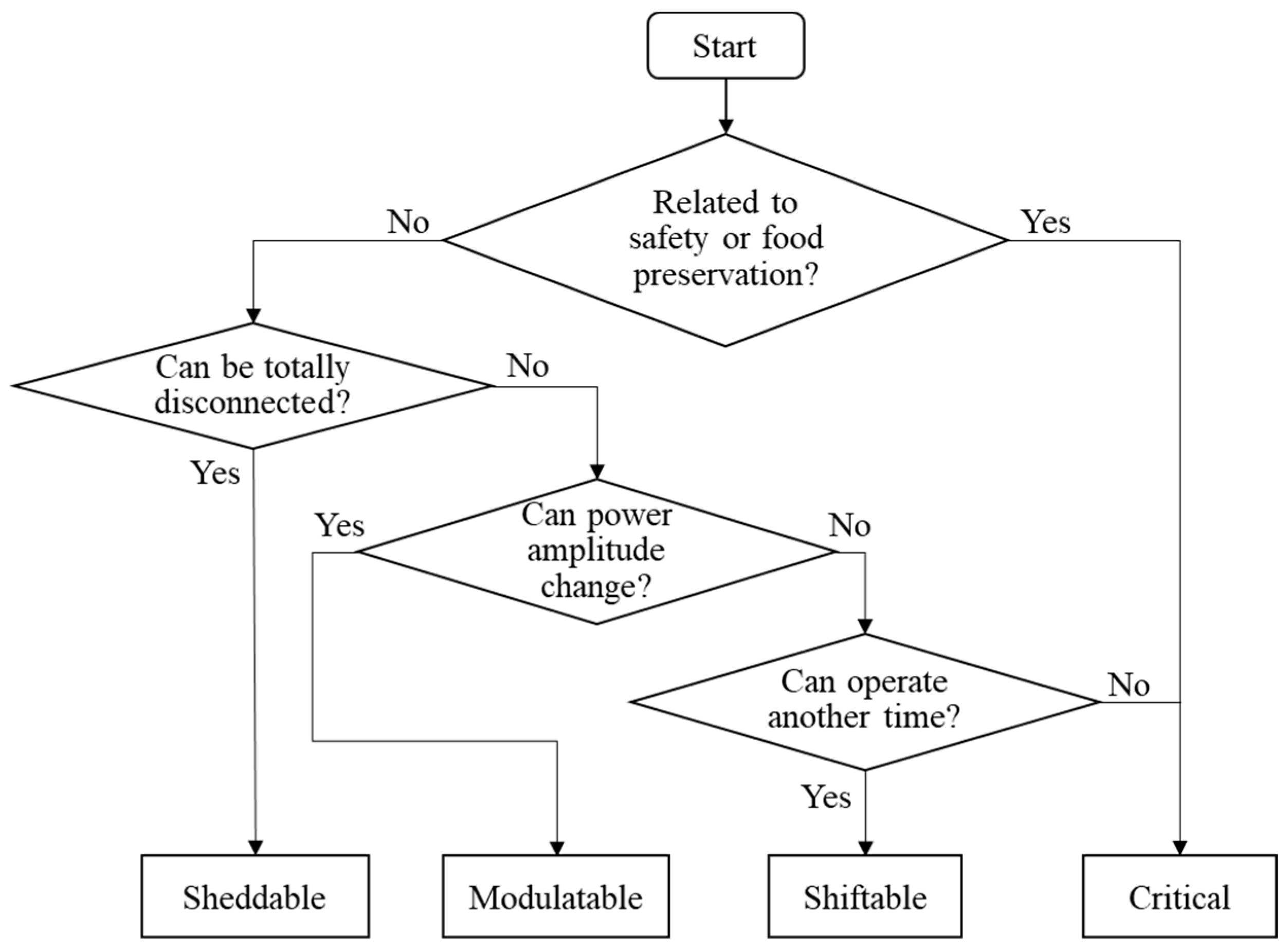
Table 3. Summary of load types in studied buildings.

Load Type	Residential	Ice Cream Shop	Bakery
Sheddable	Computer	Coffee maker, soda dispenser, outdoor ice storage	Microwave
Modulatable	HVAC	HVAC	Mixer, unspecified room plugs, HVAC
Shiftable	Range, washer, dryer	None	Range, oven, dishwasher
Critical	Lights, refrigerator	Lights, cooler, display case	Lights, cooler, display case

summarizes the load categorization results following the classification proposed in Section 2.2. In this study, we determine whether a load is sheddable from the building owner’s perspective. For instance, the coffee maker and the soda dispenser in the ice cream shop are classified as sheddable during the outage. Mixers with variable speed options, as well as the HVAC system, are classified as modulatable loads due to their varying power amplitudes. Since some plug loads in the dataset are unspecified, we sum those loads into one modulatable load. The washer, dryer, and stovetop range are considered shiftable loads in this work as their operation schedules can be flexible if needed. Lights, coolers, and display cases are classified as critical because they are related with occupants’ need for safety and food preservation. Due to the islanded circumstances, some loads commonly categorized as critical are considered to be sheddable (e.g., computer) in this paper.

Parameters related to battery configuration and penalty coefficients are summarized in

Table 4. Parameters of battery configuration and penalty coefficients.

Parameter	Residential	Ice Cream Shop	Bakery
$\mathrm{Battery}\mathrm{energy}\mathrm{upper}\mathrm{bound}{\overline{E}}_{bat}$ (kWh)	70	270	280
$\mathrm{Maximum}\mathrm{charging}\mathrm{power}{\overline{P}}_{bat}$ (kW)	28	108	112
$\mathrm{Penalty}\mathrm{of}\mathrm{charging}\gamma$	1.00 × 10−3	1.00 × 10−6	1.00 × 10−4
$\mathrm{Penalty}\mathrm{of}\mathrm{curtailment}{\gamma }^{\prime }$	5.00 × 10−3	1.00 × 10−5	1.00 × 10−3

. We assumed the maximum charging/discharging power ${\overline{P}}_{bat}$ to be 40% of the battery energy bound ${\overline{E}}_{bat}$. Further, the initial battery SOC is assumed to be 50% of ${\overline{E}}_{bat}$. The charging/discharging efficiencies are ${\eta }_{ch}={\eta }_{dis}=0.9$.

4.2. Validation of the Chance Constraint

Before further evaluating the simulation results, we first need to validate the chance constraints. The normally distributed error we introduced into outdoor temperature forecast is assumed to be $T_{amb,e}^t~\mathcal{N}\left(0,{\left(0.2\right)}^2\right)$ and the solar irradiance forecast error is assumed to be $Q_{sol,e}^t~\mathcal{N}\left(0,{\left(0.01\right)}^2\right).$ The tolerance ${\epsilon }_T$ is 0.05, meaning that with the given error distribution of forecast, the temperature range can be violated 5% of the time in the independent experiments.

Monte Carlo simulations were adopted for the constraint validation. For each timestep of the simulation, normally distributed errors were generated randomly for 1000 times and then added into the temperature prediction model in Equation (21) with the optimal HVAC operation decisions. Results showed that all temperature predictions of 10 scenarios in all three buildings are within the range of 20–28 $°\mathrm{C}$. As an example, Figure 3 compares the temperature predictions with and without uncertainty using the simulation results for scenario S11. We see that, with the accumulation of prediction errors (both positive and negative), the absolute difference between the temperature trajectories with and without forecast error lies within the 0–0.5 $°\mathrm{C}$ range.

4.3. Impact of Weighting Factor

This section first discusses the allocation factors ${\alpha }_i^t$ generated by the operator layer, which later serves as the input for the smart controllers at the building layer. Then, we compare the scheduled load shapes, battery behavior, and indoor temperature of each building in different scenarios to further discuss the impact of weighting factors on the KPIs.

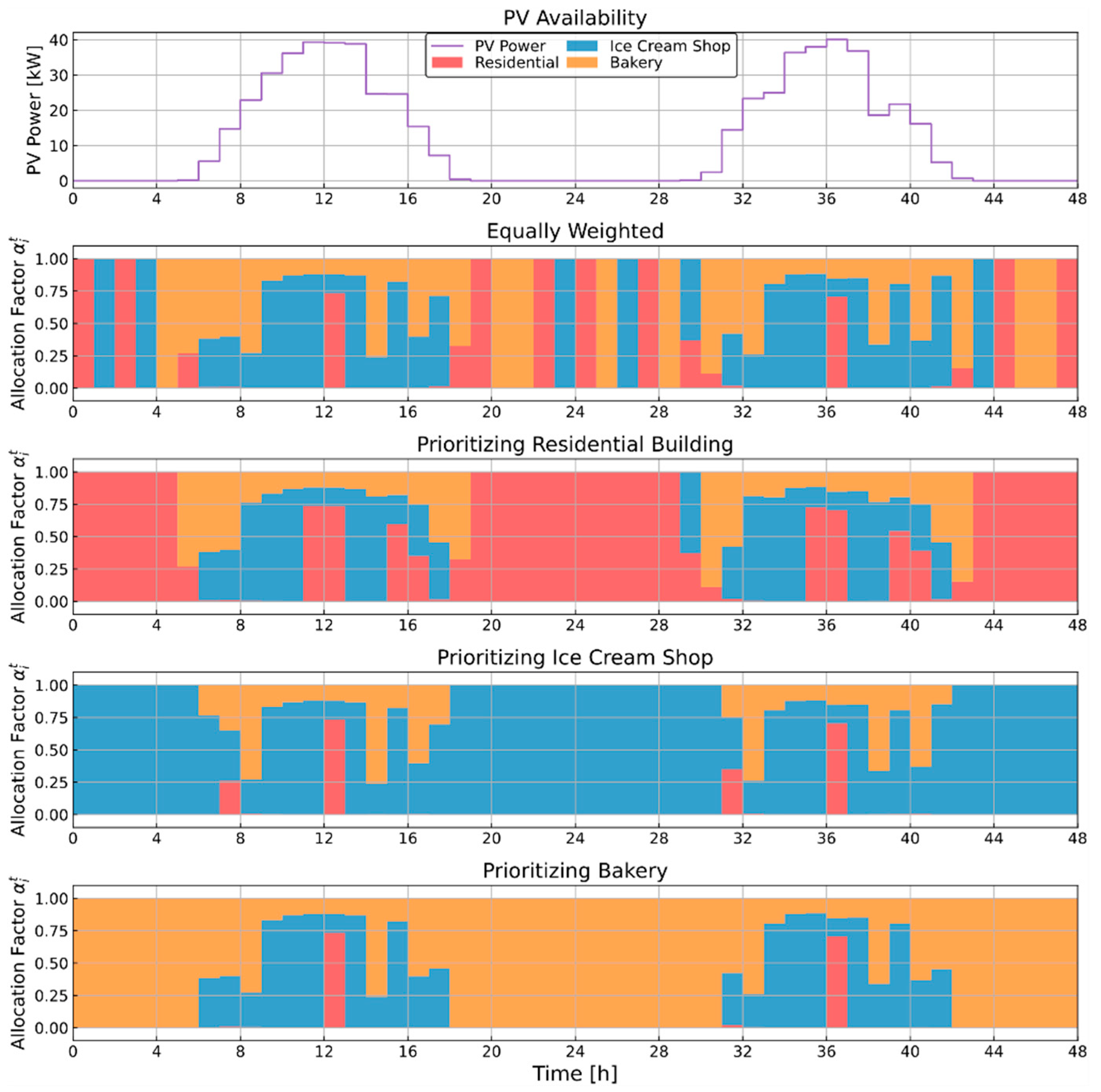
Figure 4 compares the allocation factors for equally weighted buildings (baseline) with weightings that prioritize each building over the others. Qualitatively, when all buildings are equally weighted in the allocation process (second plot from top), we see a rather random behavior for the PV allocation during the nighttime when no PV power is available. All three buildings take turn to get full PV power (${\alpha }_i^t=1$) because they have the same objective function value. On the contrary, for the scenarios when single building is prioritized, the prioritized building gets full PV power alone during the nighttime (bottom three plots). During the daytime, when more PV generation is available, the allocation results follow similar trends for all scenarios regardless of the weighting method. Although generally we see less load shedding in the prioritized building, as well as a higher value of the allocation factor, the allocation process is mostly constrained by the building load flexibility ranges. More specifically, buildings with a higher load flexibility lower bound (i.e., ice cream shop) tend to get more allowable load than other buildings.

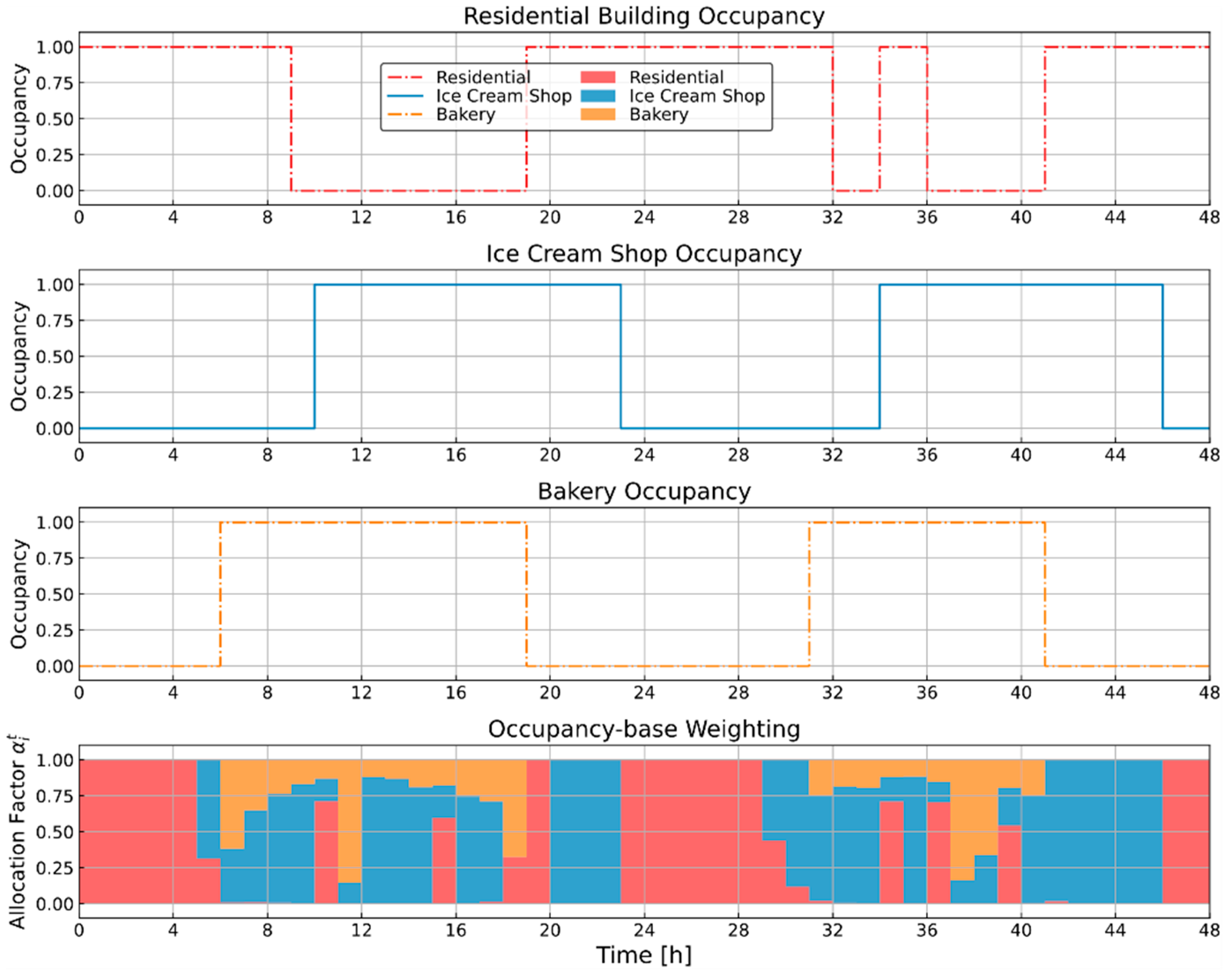
Figure 5 plots the allocation factors for occupancy-based weighting method against building occupancy. Here, occupancy indicates whether the building is occupied. In this work, we do not consider number of people in the building as we don’t have access to this level of data. From the middle plot, we see that the residential building is mostly occupied during the night from about 7 P.M. to 8 A.M. Ice cream shop and bakery are occupied during the day from 10 A.M.–11 P.M. and 6 A.M.–7 P.M., respectively. From the bottom plot, we see that similar to single building prioritized scenarios, when at night only residential building is occupied, it gets full PV allocation. However, when the time reaches 5 A.M., the allocation factor of the residential building starts to decrease and during the day only a few hours will it get PV power due to its unoccupied status. During the daytime, when both the bakery and ice cream shop are occupied, the allocation basically follows the buildings’ power flexibility lower bounds as discussed before.

To further quantify the impact of different weighting methods, the mean values of the allocation factors $\overline{{\alpha }_i^t}$, as well as the total allocated PV energy are listed in

Table 5. Mean values of allocation factors and PV energy allocation for different weighting methods.

Building	Equal Weighting		Priority-Based Weighting						Occupancy-Based Weighting
			Prioritize Residential		Prioritize Ice Cream Shop		Prioritize Bakery
	$\overline{{\mathit{\alpha }}_{\mathit{i}}^{\mathit{t}}}$	${\mathit{E}}_{\mathit{p}\mathit{v}}\left(\mathit{k}\mathit{W}\mathit{h}\right)$	$\overline{{\mathit{\alpha }}_{\mathit{i}}^{\mathit{t}}}$	${\mathit{E}}_{\mathit{p}\mathit{v}}\left(\mathit{k}\mathit{W}\mathit{h}\right)$	$\overline{{\mathit{\alpha }}_{\mathit{i}}^{\mathit{t}}}$	${\mathit{E}}_{\mathit{p}\mathit{v}}\left(\mathit{k}\mathit{W}\mathit{h}\right)$	$\overline{{\mathit{\alpha }}_{\mathit{i}}^{\mathit{t}}}$	${\mathit{E}}_{\mathit{p}\mathit{v}}\left(\mathit{k}\mathit{W}\mathit{h}\right)$	$\overline{{\mathit{\alpha }}_{\mathit{i}}^{\mathit{t}}}$	${\mathit{E}}_{\mathit{p}\mathit{v}}\left(\mathit{k}\mathit{W}\mathit{h}\right)$
Residential	0.099	59.52	0.218	153.85	0.075	67.18	0.054	58.67	0.163	108.61
Ice Cream Shop	0.499	350.07	0.455	309.51	0.669	356.00	0.454	346.20	0.581	308.51
Bakery	0.402	169.08	0.326	115.31	0.256	155.50	0.492	173.80	0.255	161.56

. Due to the highly stochastic allocation during nighttime when no PV power is available, we only counted hours when PV generation is greater than zero in the calculation of $\overline{{\alpha }_i^t}$. From the table, we noticed that having a lower mean allocation factor does not necessarily mean less PV energy allocation. For example, in the scenario where the residential building is prioritized, its $\overline{{\alpha }_i^t}$ is less than 22% while for the bakery it is almost 33%. However, the total PV energy allocated to the residential building is 33.42% more than that allocated to the bakery. This is because the residential building has higher ${\alpha }_i^t$ values during hours with the most PV generation (i.e., around noon). This indicates that having a higher allocation factor when more PV power is generated is more crucial. When looking at the occupancy-based weighting scenario, the residential building PV energy exceeds that of the equal weighting scenario since the shortly occupied hours during the day (e.g., hours 34–36) bring more allocation. Overall, no matter which weighting method is adopted, the ice cream shop is always allocated the most PV energy due to its large refrigeration loads, while the residential building is always allocated the least amount of PV energy (except when it is prioritized in scenarios S21_R and S22_R). This indicates that the impact of power flexibility is more prominent than the weighting factors during the resource allocation.

Next, the simulation results will be discussed for the various PV allocation methods. In the following discussion, we highlight a subset of the results; however, the complete set of results are available in Appendix A and quantitative results for all 30 simulations are summarized in

Table A1. Detailed KPIs for each building and community overall of each scenario.

		$\mathbf{Temperature}\mathbf{Deviation}(°\mathbf{C})$	PV Curtailment Ratio	Unserved Load Ratio					Battery Size (kWh)
				Sheddable	Shiftable	Modulatable	Critical	Overall
S11	R	1.34	0.00%	0.00%	19.92%	N/A	0.00%	5.99%	34.71
	I	2.62	0.00%	0.00%	N/A	N/A	0.00%	0.00%	89.81
	B	0.77	0.00%	0.00%	8.18%	0.00%	0.00%	0.38%	75.28
	Community	3.04	0.00%	0.00%	10.94%	0.00%	0.00%	0.27%	199.80
S21_R	R	2.76	31.25%	0.00%	19.92%	N/A	0.00%	5.99%	45.57
	I	2.65	0.00%	0.00%	N/A	N/A	0.00%	0.00%	75.85
	B	1.34	0.00%	0.00%	8.18%	0.00%	0.00%	0.38%	94.13
	Community	4.05	8.31%	0.00%	10.94%	0.00%	0.00%	0.27%	215.55
S21_I	R	0.79	0.00%	0.00%	19.92%	N/A	0.00%	5.99%	35.56
	I	2.62	0.00%	0.00%	N/A	N/A	0.00%	0.00%	93
	B	0.50	0.00%	0.00%	8.18%	0.00%	0.00%	0.38%	81.08
	Community	2.78	0.00%	0.00%	10.94%	0.00%	0.00%	0.27%	209.64
S21_B	R	1.45	0.00%	0.00%	19.92%	N/A	0.00%	5.99%	35.56
	I	2.62	0.00%	0.00%	N/A	N/A	0.00%	0.00%	87.79
	B	0.79	0.00%	0.00%	8.18%	0.00%	0.00%	0.38%	71.26
	Community	3.10	0.00%	0.00%	10.94%	0.00%	0.00%	0.27%	194.61
S31	R	2.06	5.50%	0.00%	19.92%	N/A	0.00%	5.99%	38.79
	I	2.69	0.00%	0.00%	N/A	N/A	0.00%	0.00%	77.67
	B	0.80	0.00%	0.00%	8.18%	0.00%	0.00%	0.38%	66.45
	Community	3.48	1.03%	0.00%	10.94%	0.00%	0.00%	0.27%	182.91
S12	R	0.29	0.00%	86.50%	19.92%	N/A	0.00%	10.80%	28.99
	I	0.28	0.00%	63.72%	N/A	N/A	0.00%	12.74%	124.68
	B	0.34	0.00%	99.03%	8.18%	68.89%	0.00%	4.32%	64.4
	Community	0.53	0.00%	64.14%	10.94%	68.89%	0.00%	9.25%	218.07
S22_R	R	0.29	49.57%	31.49%	19.92%	N/A	0.00%	7.74%	39.81
	I	0.28	0.00%	65.17%	N/A	N/A	0.00%	13.03%	90.25
	B	0.34	0.00%	100.00%	8.18%	77.00%	0.00%	4.77%	111.99
	Community	0.53	13.18%	65.06%	10.94%	77.00%	0.00%	9.54%	242.05
S22_I	R	0.29	0.00%	85.89%	19.92%	N/A	0.00%	10.77%	32.82
	I	0.28	0.00%	63.72%	N/A	N/A	0.00%	12.74%	127.86
	B	0.34	0.00%	99.03%	8.18%	72.83%	0.00%	4.54%	77.23
	Community	0.53	0.00%	64.13%	10.94%	72.83%	0.00%	9.34%	237.91
S22_B	R	0.29	0.00%	86.50%	19.92%	N/A	0.00%	10.80%	28.37
	I	0.28	0.00%	63.72%	N/A	N/A	0.00%	12.74%	122.66
	B	0.34	0.00%	99.03%	8.18%	69.23%	0.00%	4.34%	59.16
	Community	0.53	0.00%	64.14%	10.94%	69.23%	0.00%	9.26%	210.19
S32	R	0.29	28.93%	46.01%	19.92%	N/A	0.00%	8.55%	35.33
	I	0.28	0.00%	65.47%	N/A	N/A	0.00%	13.09%	90.88
	B	0.34	0.00%	100.00%	8.18%	73.64%	0.00%	4.58%	73.31
	Community	0.53	5.43%	65.49%	10.94%	73.64%	0.00%	9.51%	199.52

. In the following simulation results, the baseline power is the original load shape from data. The positive battery power means charging and negative means discharging. The scheduled sheddable, modulatable, shiftable loads, and critical loads are represented by color blocks. When evaluating the thermal comfort results, the baseline temperature is the original indoor temperature with a setpoint of 24 °C without optimization. For clarity, the label S21 in the temperature plots represents the scenario of the discussed building being prioritized, as described in Table 1.

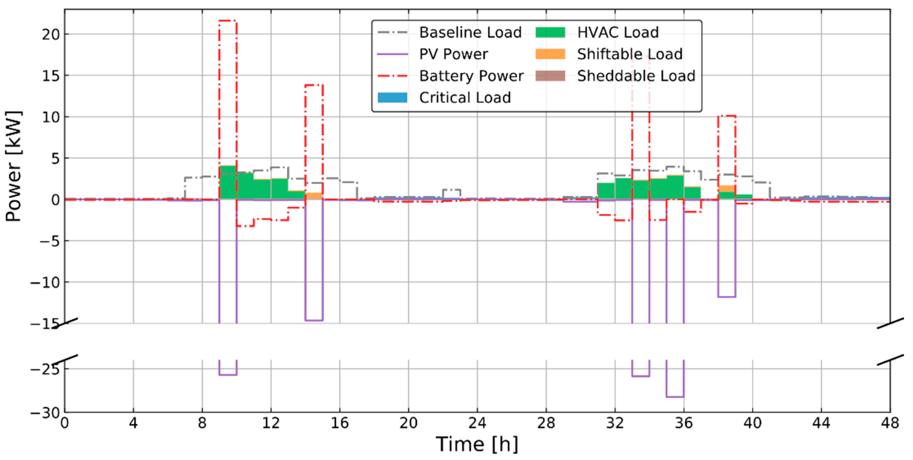
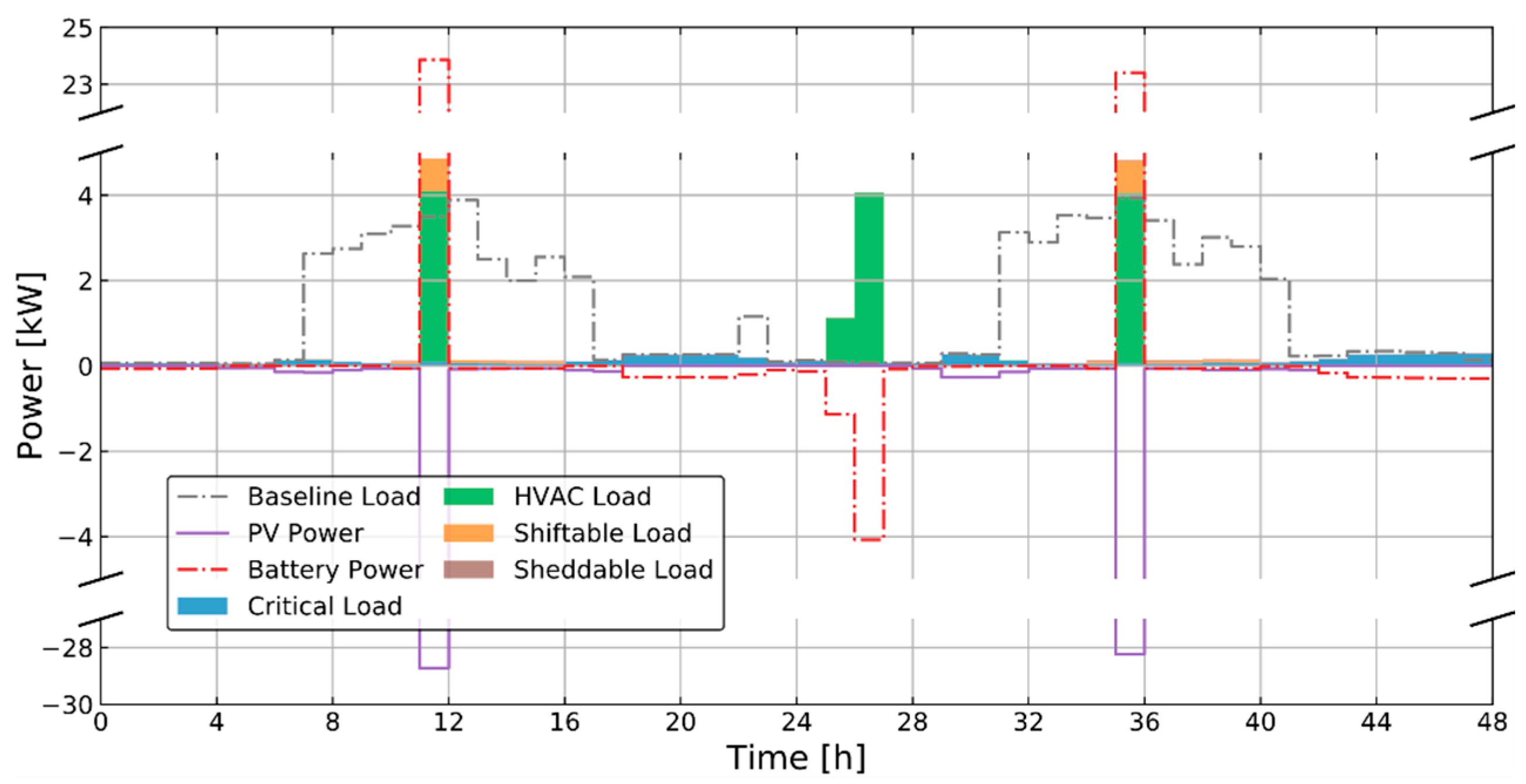
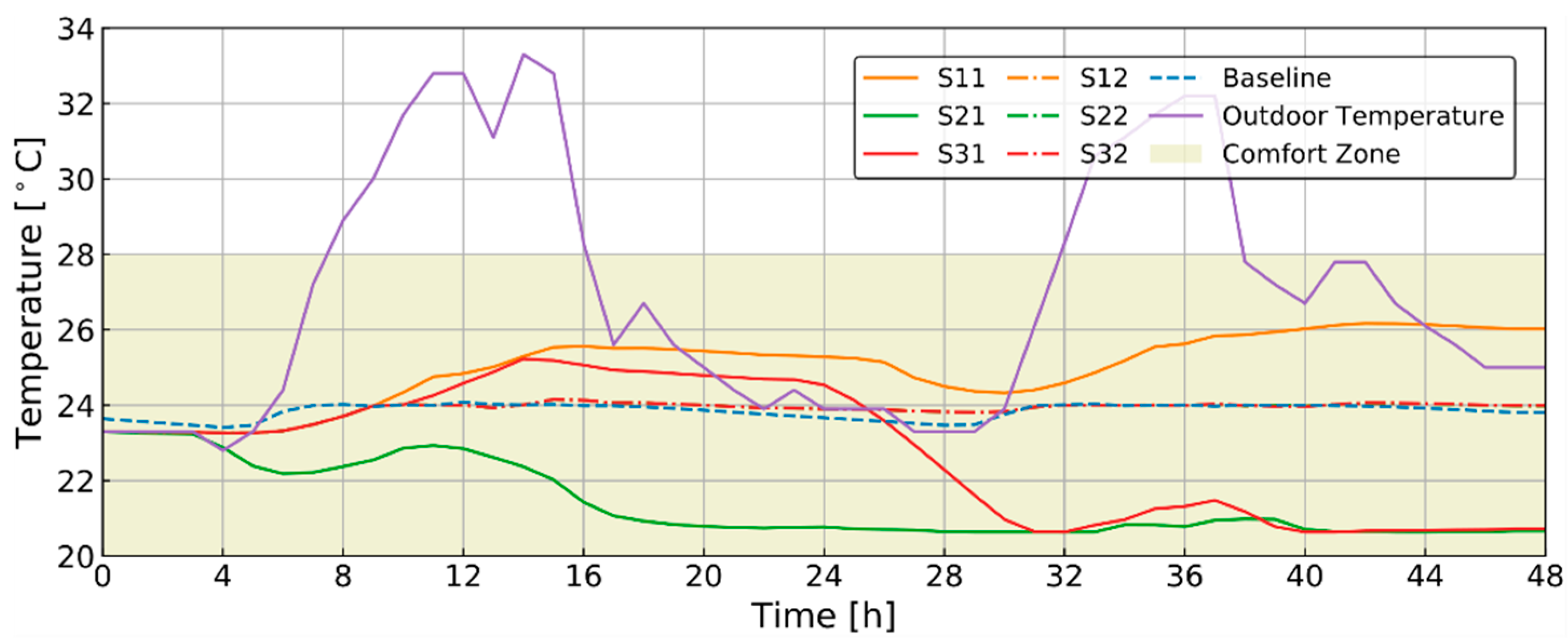
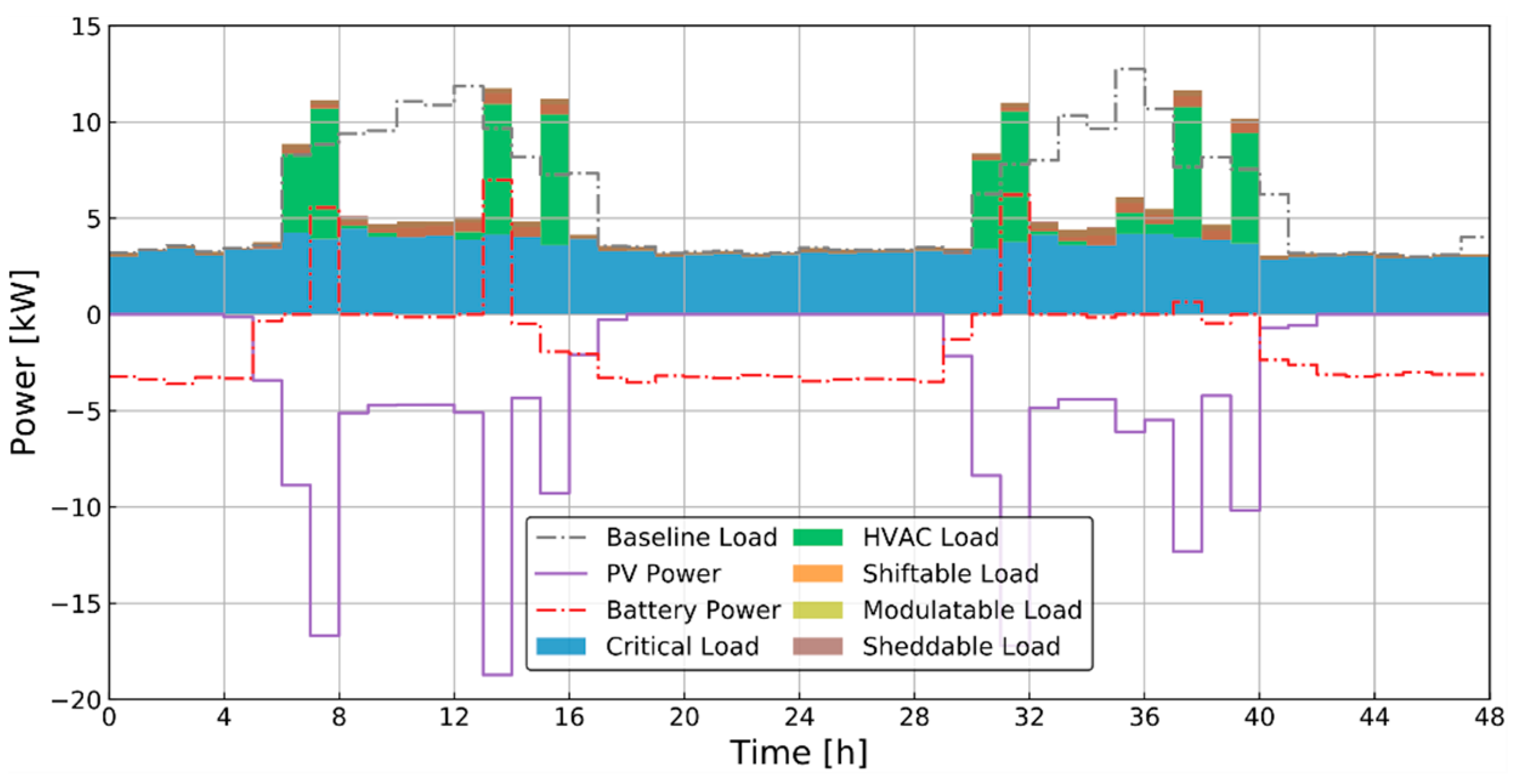
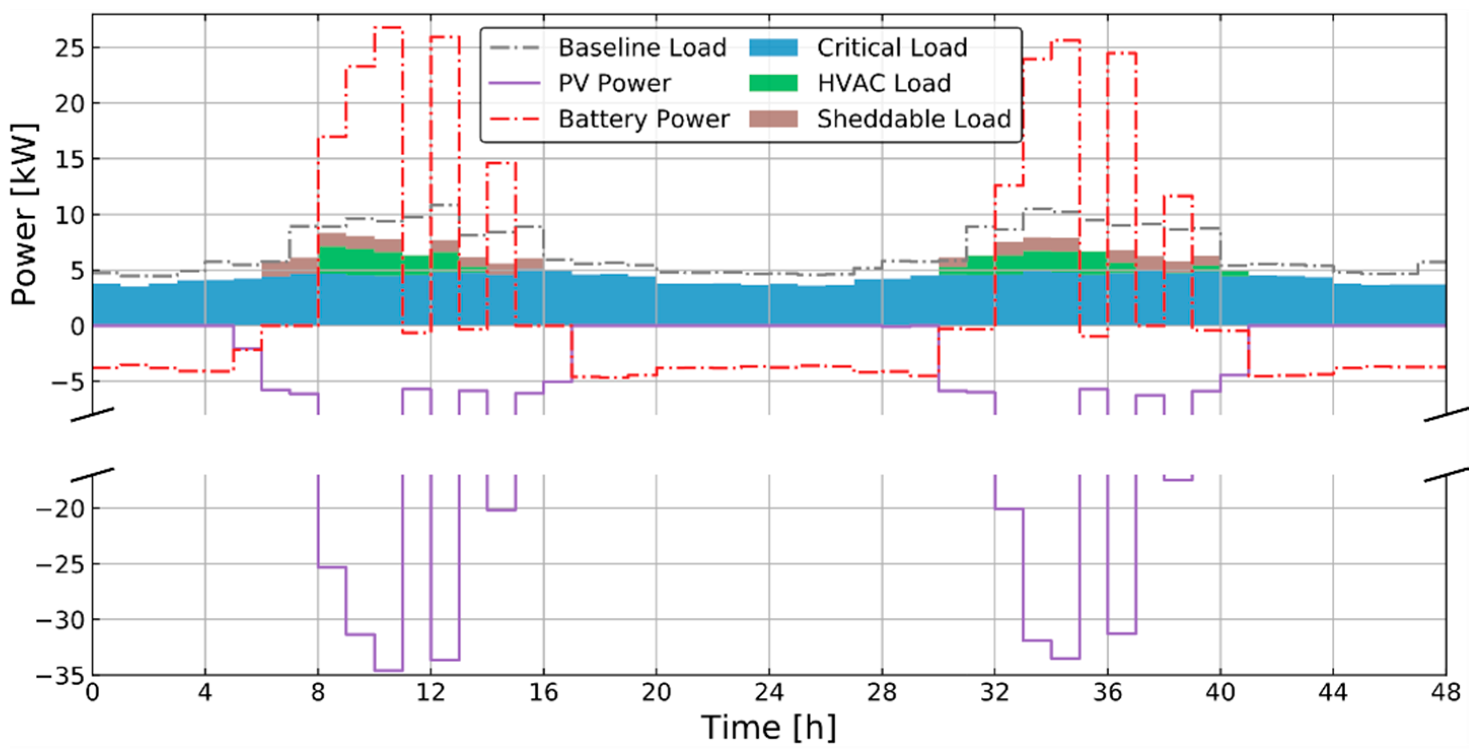
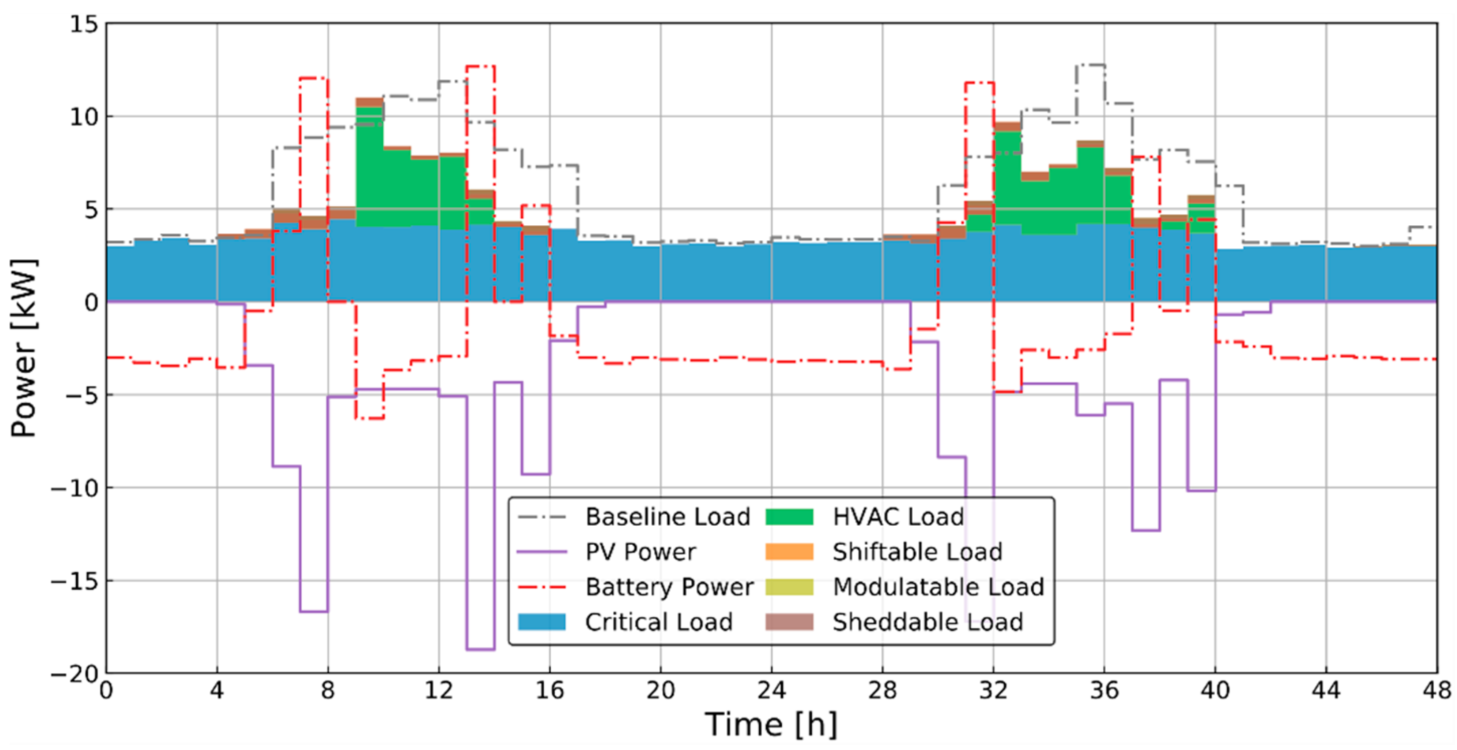
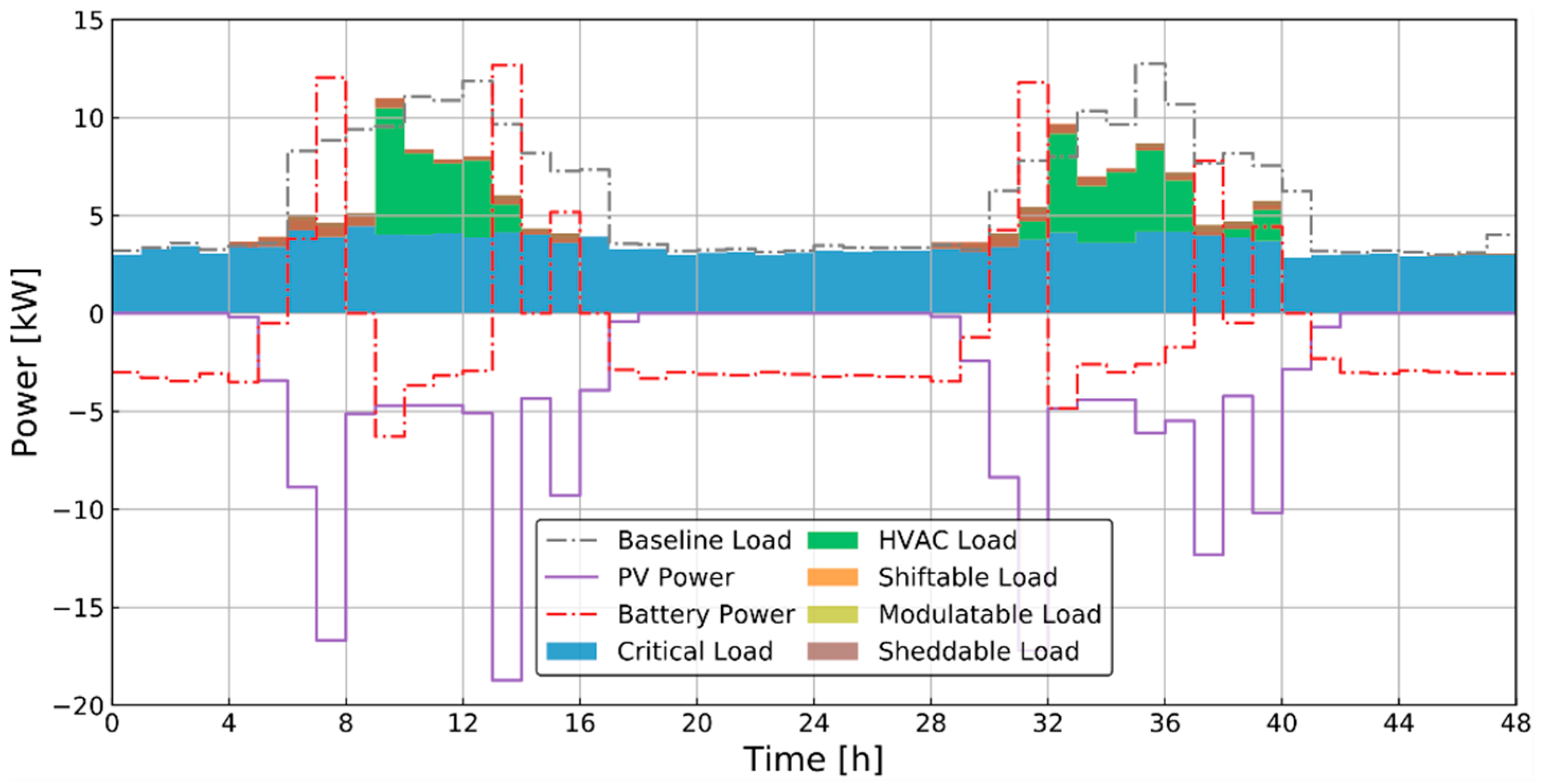
The residential building operation is compared in the scenario where all buildings are equally weighted and where the residential building is prioritized in Figure 6 and Figure 7, respectively. In both scenarios, we see that shiftable loads are scheduled during the day when more PV power is available. All sheddable and modulatable loads are satisfied in both cases (see Table A1 for details). When the allocated PV power is more than doubled in the residential building due to it being prioritized, we see more battery charging and discharging in Figure 7. However, more than enough PV power is allocated to the residential building in this case due to its high priority, resulting in 31.25% of the allocated PV power being curtailed. 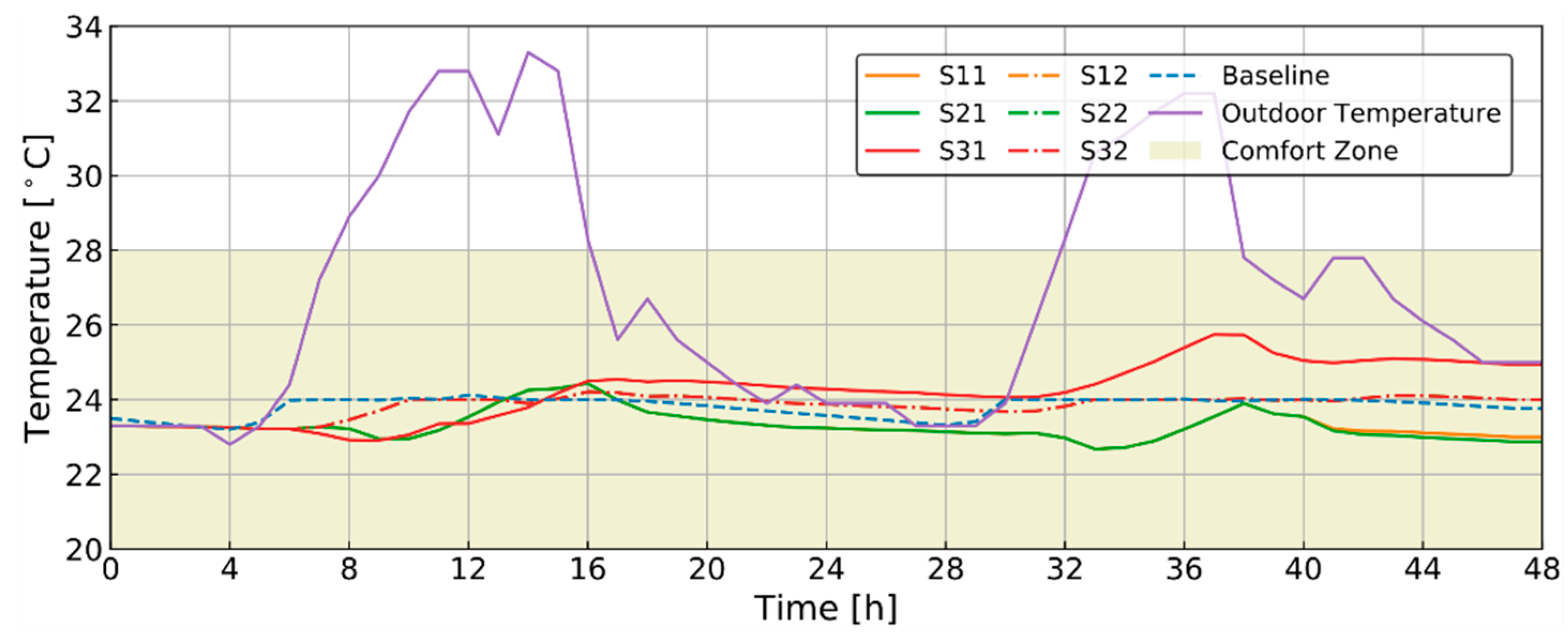Additionally, more power is allocated to the HVAC system in Figure 7, causing the indoor temperature to be closer to the lower bound (Figure 8). Comparing S11, S21, S31 with various weighting factors in Figure 8, we see that scenarios with more allocated PV power results in a lower indoor temperature since more power is available for the HVAC load. In Figure 8, all temperatures are within the comfort bounds. It is noted that in Figure 8, S12, S22, and S32 temperature curves have almost the same trend that they cannot be differentiated from the plot.

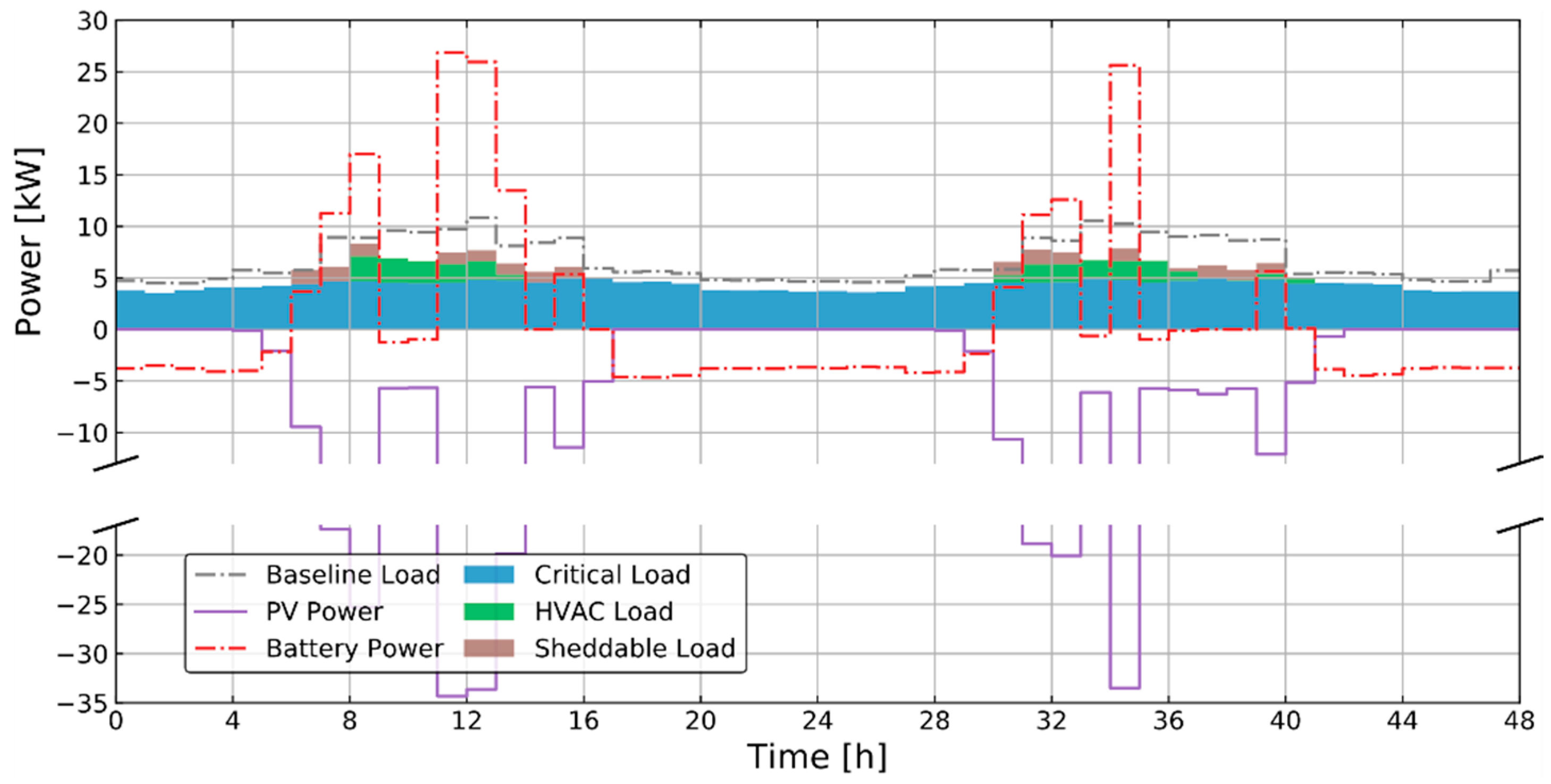
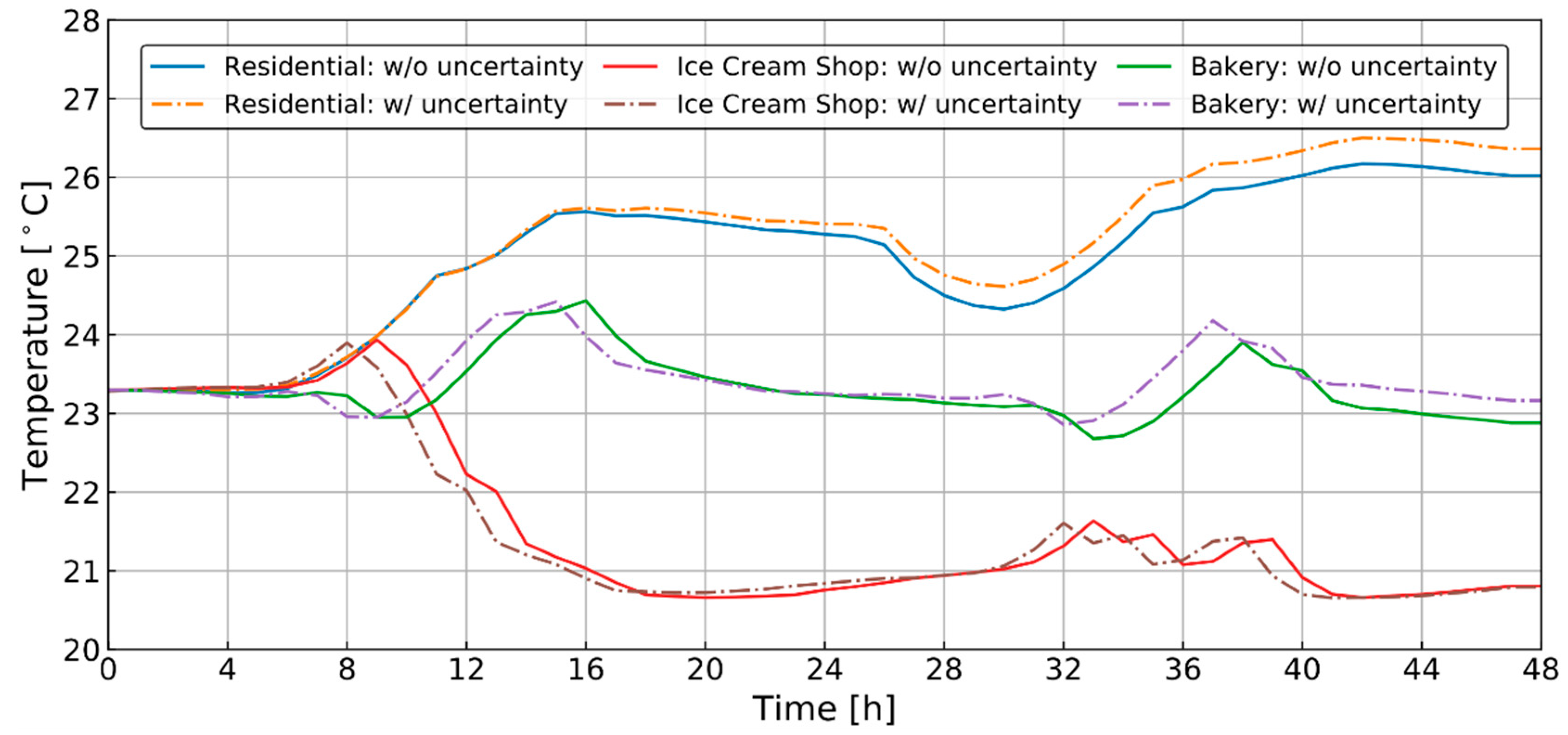
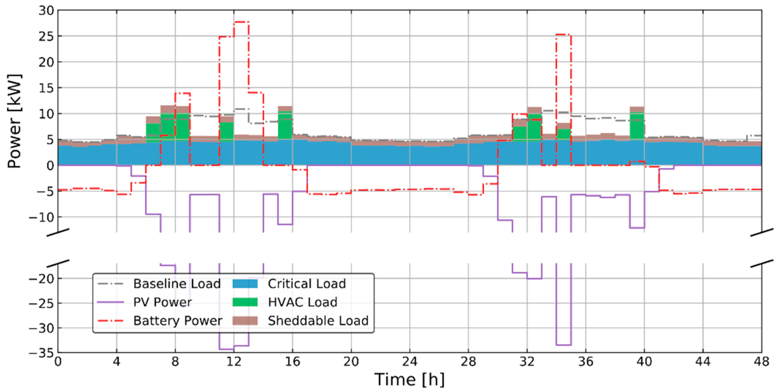
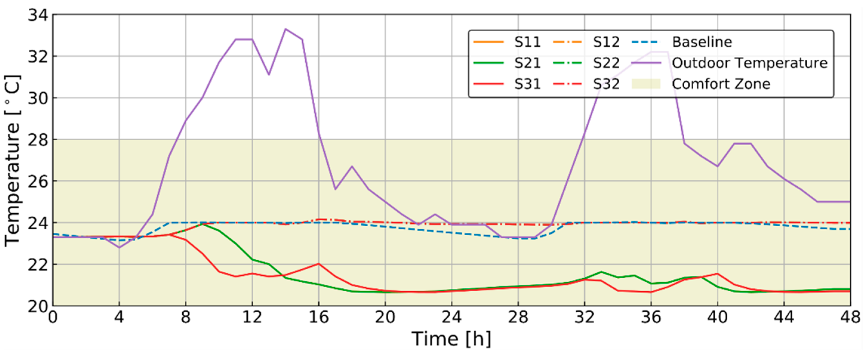
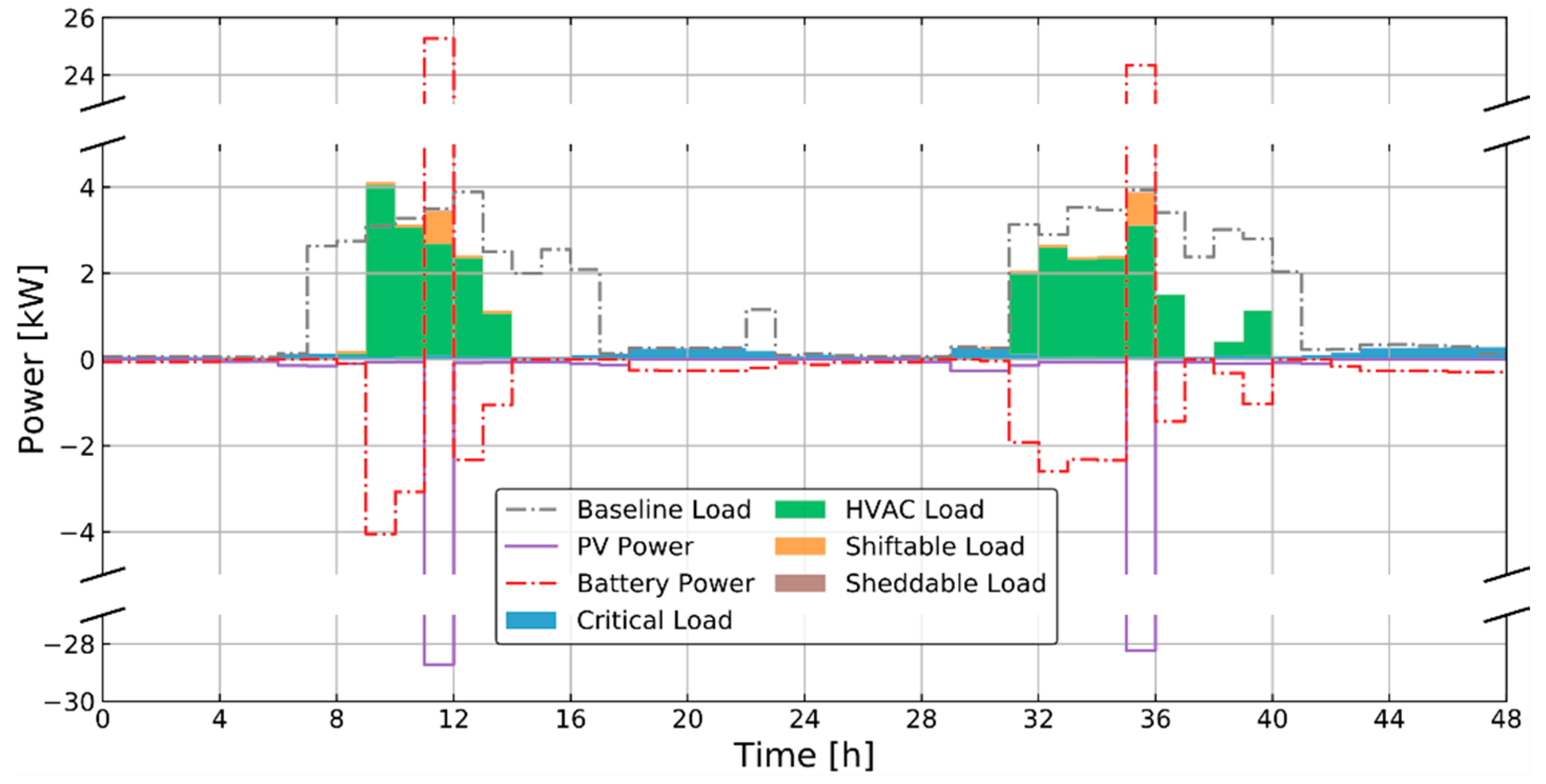
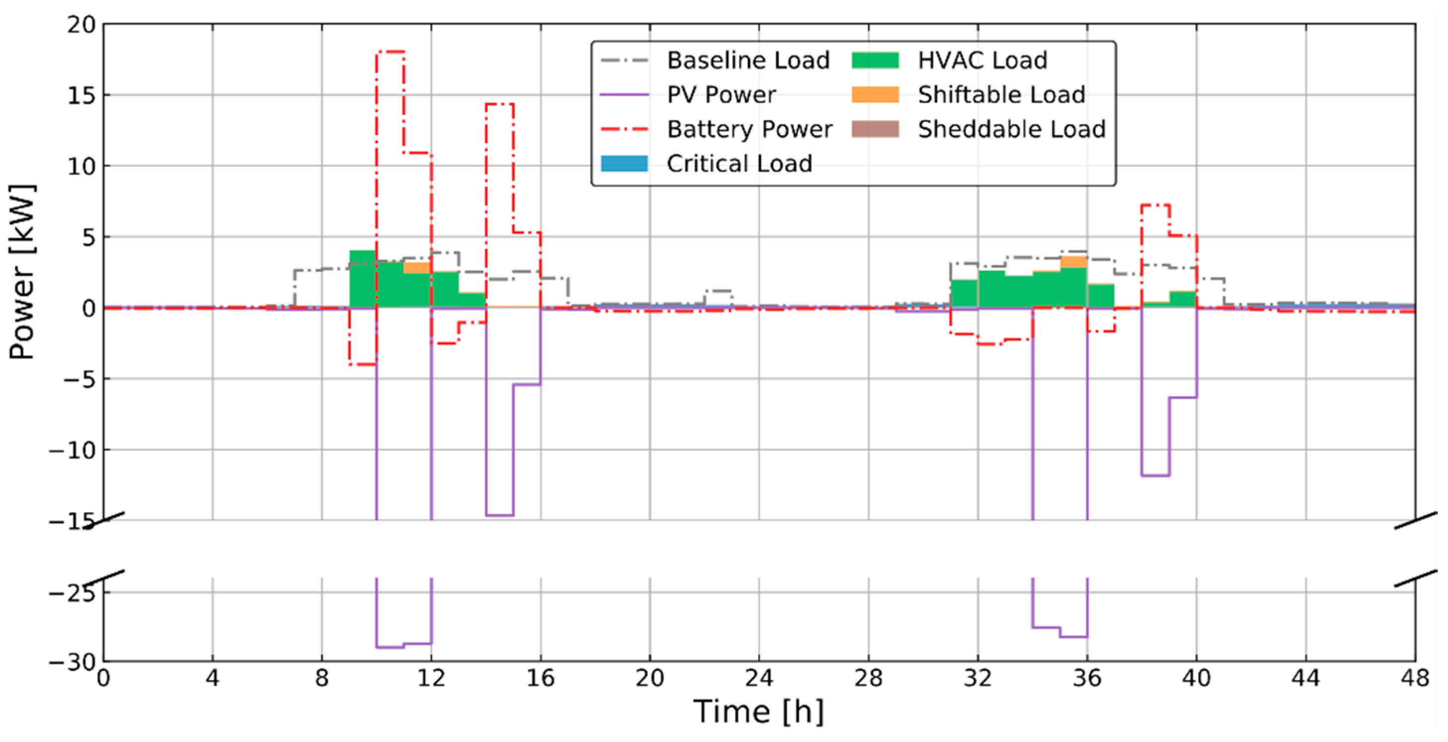
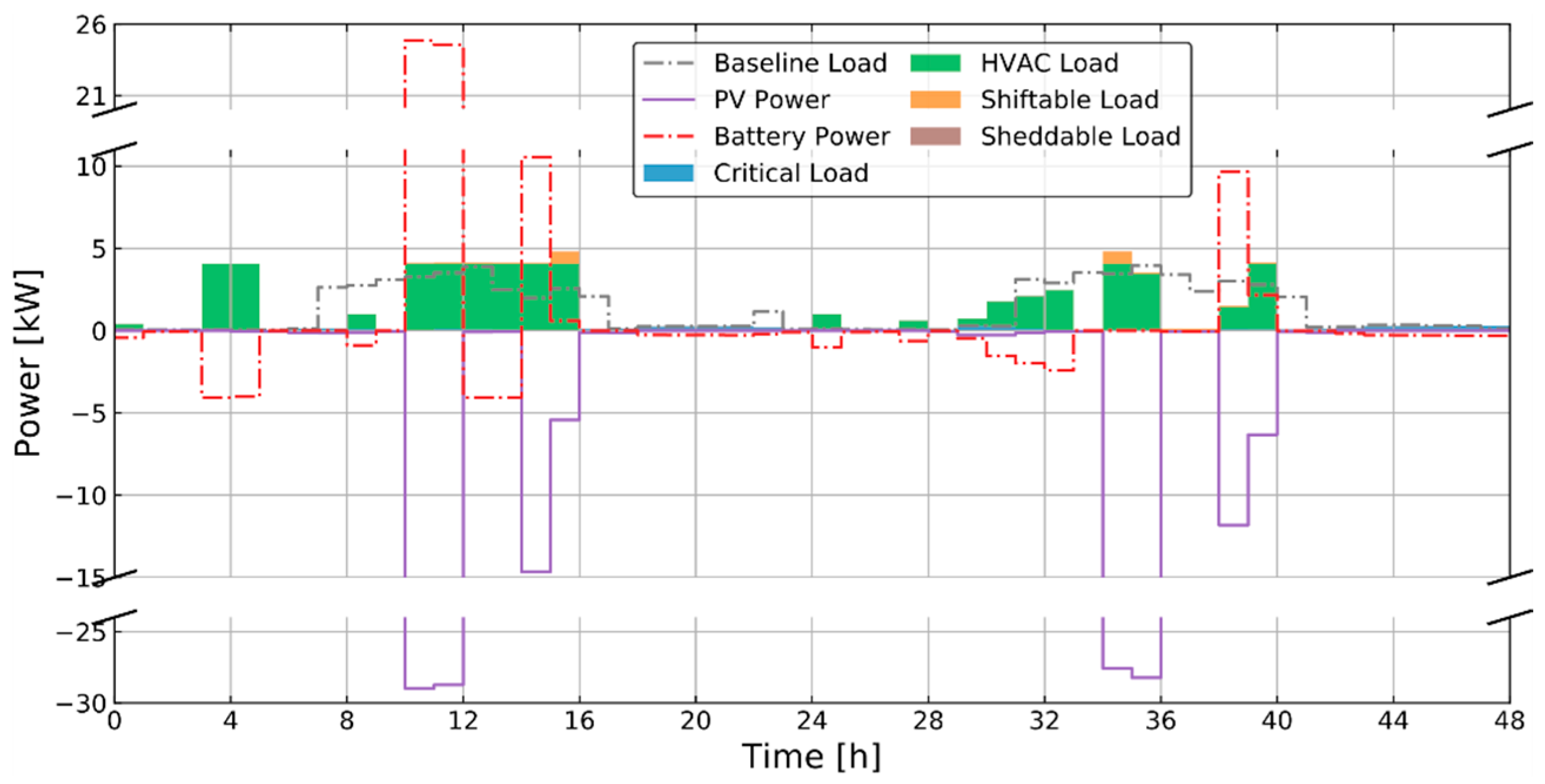
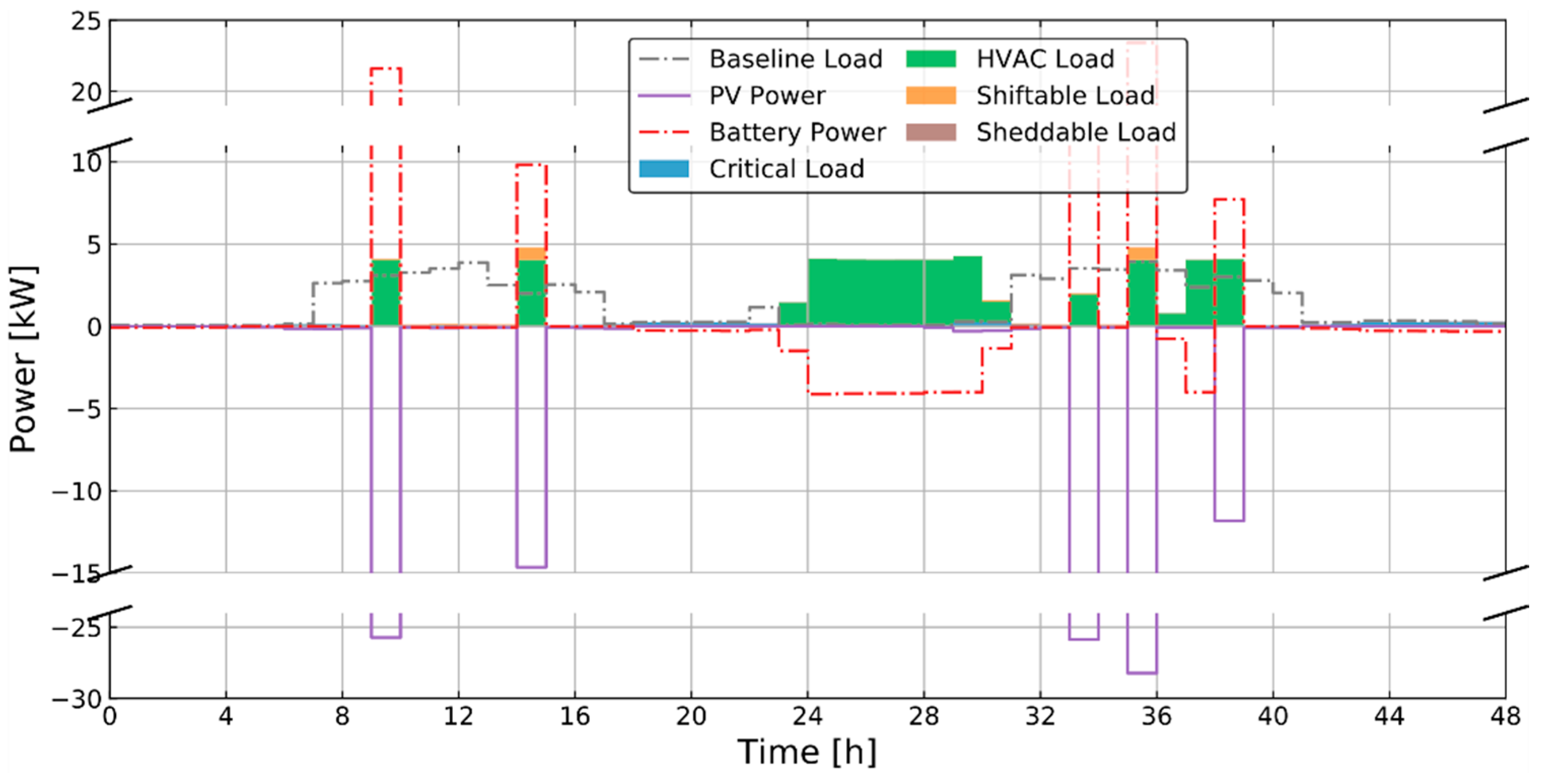
Figure 9 depicts the results for the ice cream shop with equal weighting while Figure 10 shows the results with occupancy-based weighting. Since the total allocated PV energy in Figure 10 is reduced by about 12% that compared to Figure 9, we see much less battery charging and a slight reduction of HVAC power in Figure 10. All sheddable loads are satisfied in both cases (see Table A1 for details). In Figure 11, the indoor temperature trajectories of S11 and S21 overlap with each other as almost the same amount of PV power is allocated to the ice cream shop in these two scenarios. The indoor temperature in simulation scenario S31 first drops below those of scenarios S11 and S21 in the morning due to a precooling between 6 to 9 A.M., and then exceeds them in the afternoon due to less power available to operate the HVAC system. A similar trend is also seen in the following simulation day. As in the residential building, Figure 11 shows that the indoor thermal comfort of the ice cream shop was maintained within the given temperature bounds. It is noted that in Figure 11, S12, S22, and S32 temperature curves have almost the same trend that they cannot be differentiated from the plot.

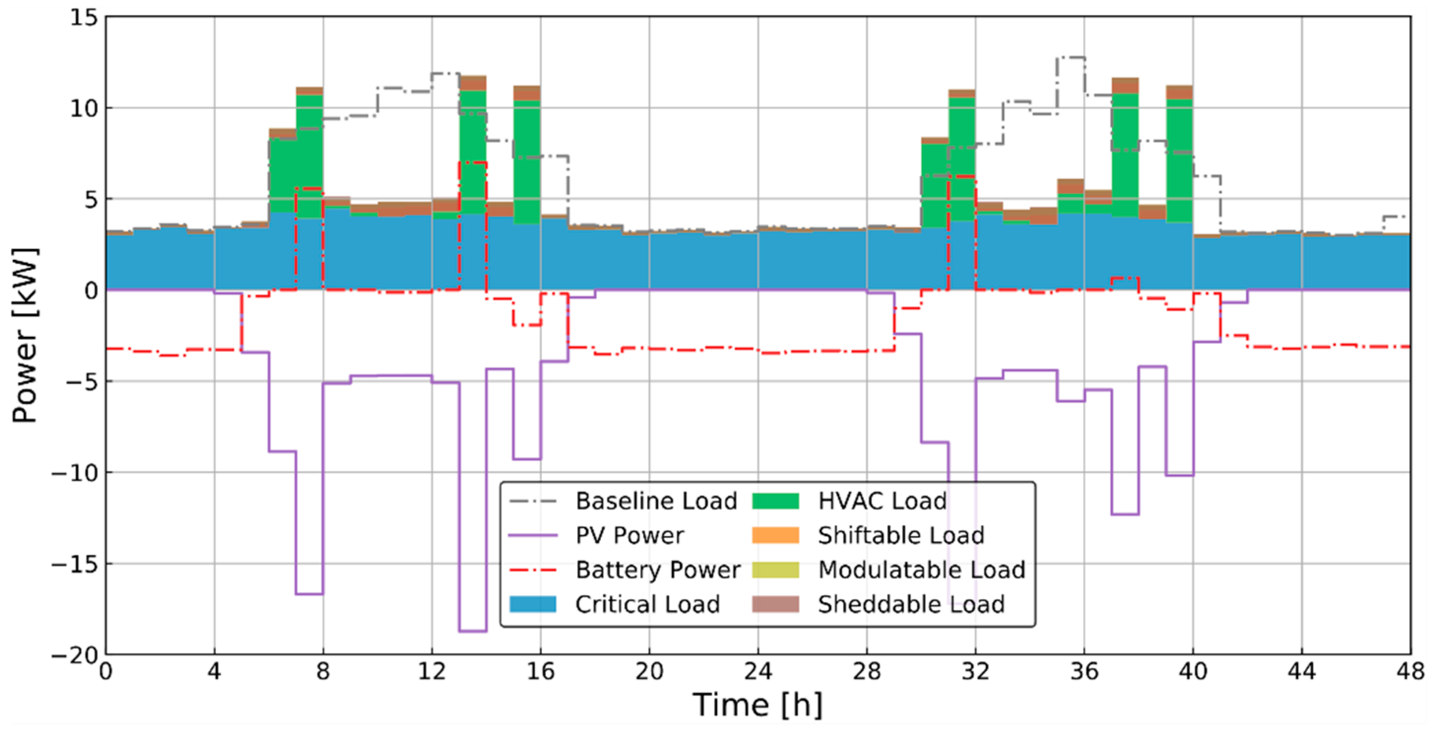
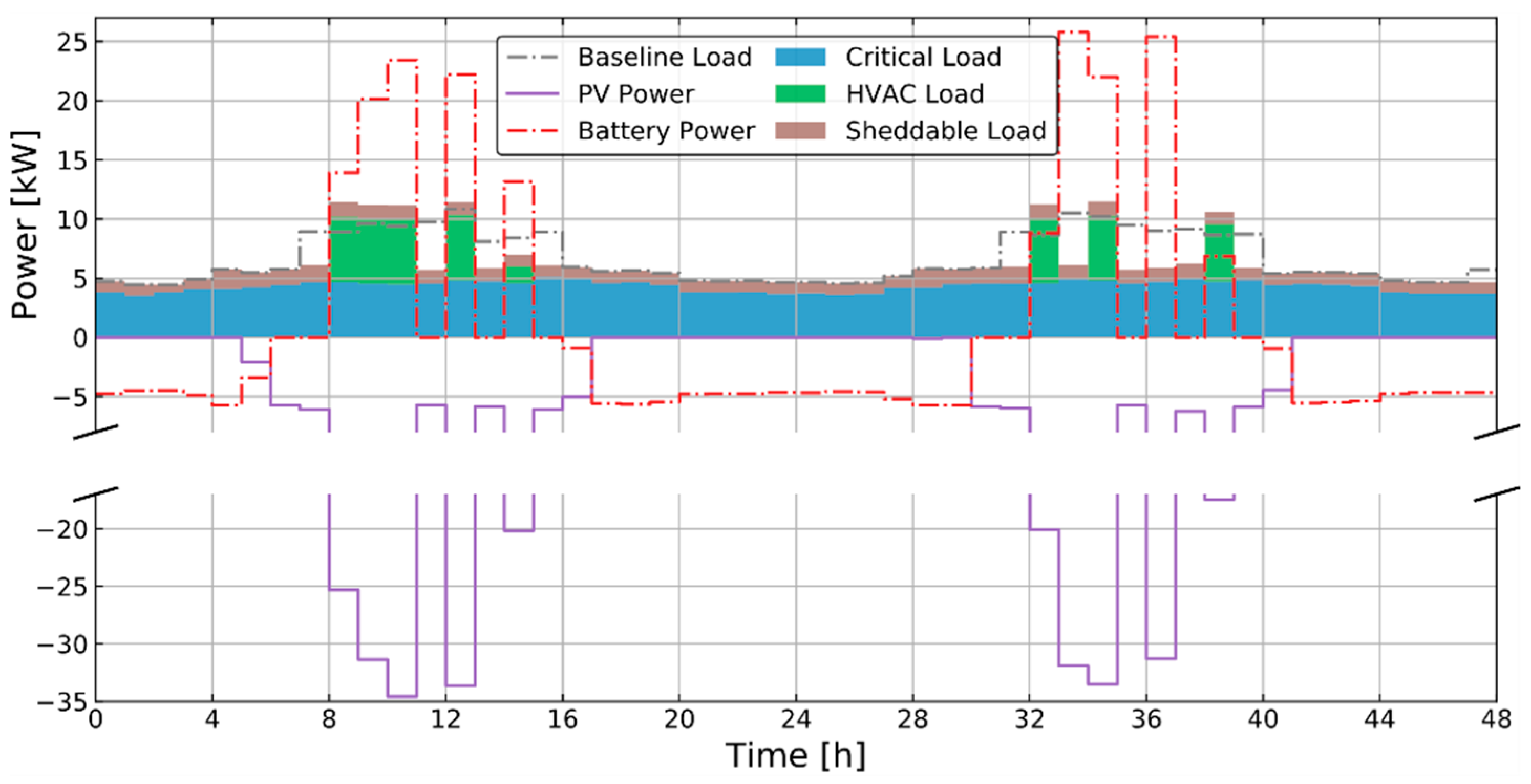
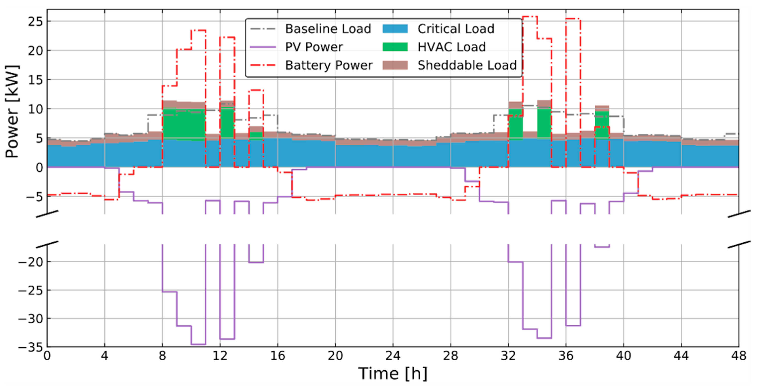
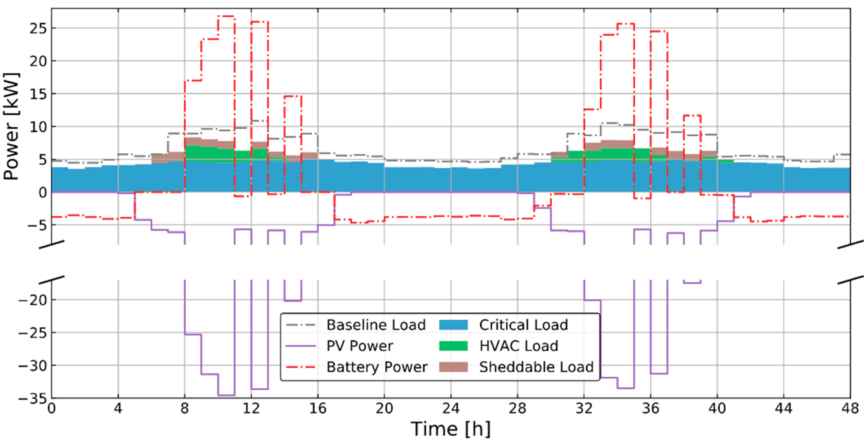
Figure 12 plots the results for bakery with equal weighting while Figure 13 with occupancy-based weighting. Due to a reduction of PV power in Figure 13, much less power is allocated to the HVAC system, especially during late afternoon (e.g., hour 16 and 40). The battery discharging is almost the same in the two scenarios, both to satisfy the four types of loads present in this building. All sheddable and modulatable loads are satisfied in both cases (see Table A1 for details). However, battery charging only happens about once a day in scenario S31 given the focused allocated PV power shape. In Figure 14, the indoor temperature for S31 is higher than S11 due to less power available to operate the HVAC system. All temperatures are within the comfort temperature bounds. It is noted that in Figure 14, S12, S22, and S32 temperature curves have almost the same trend that they cannot be differentiated from the plot.

To summarize, in this section, we discussed the PV resource allocation results under different weighting methods. The resulted load shape, battery behavior, and indoor temperatures are also discussed qualitatively. From the discussion, we found that the weighting method of the operator layer directly affects the mean allocation factor of each building. When one building is prioritized, we see an obvious increase of $\overline{{\alpha }_i^t}$. However, a higher $\overline{{\alpha }_i^t}$ does not necessarily mean more PV energy allocation. A higher allocation factor during time periods with more PV generation (e.g., around noon) is more crucial than a higher mean value of the allocation factor overall. Additionally, we noticed that the allocation process is mostly constrained by the building load flexibility ranges. More specifically, buildings with a higher load flexibility lower bound (i.e., ice cream shop with large critical loads) tend to get more allowable load than other buildings. Additionally, when prioritizing buildings according to occupancy status, the building with longer occupant presence gets more PV power, which is not necessarily a fair allocation method. For instance, in S31, 5.5% of the PV energy allocated to the residential building was curtailed. Since the allocation process was according to building occupancy time, more than enough power is allocated to the residential building in this case. Lastly, the resulting load schedule, battery behavior, and indoor temperature are directly correlated with the available PV power when other system settings are the same (e.g., battery charging constraints and penalty coefficients).

4.4. Impact of Objective Function

This section discusses the impact of different objective functions on the scheduled load shapes, battery behavior, and indoor temperature. Similar to the last section, qualitative discussions will first be provided.

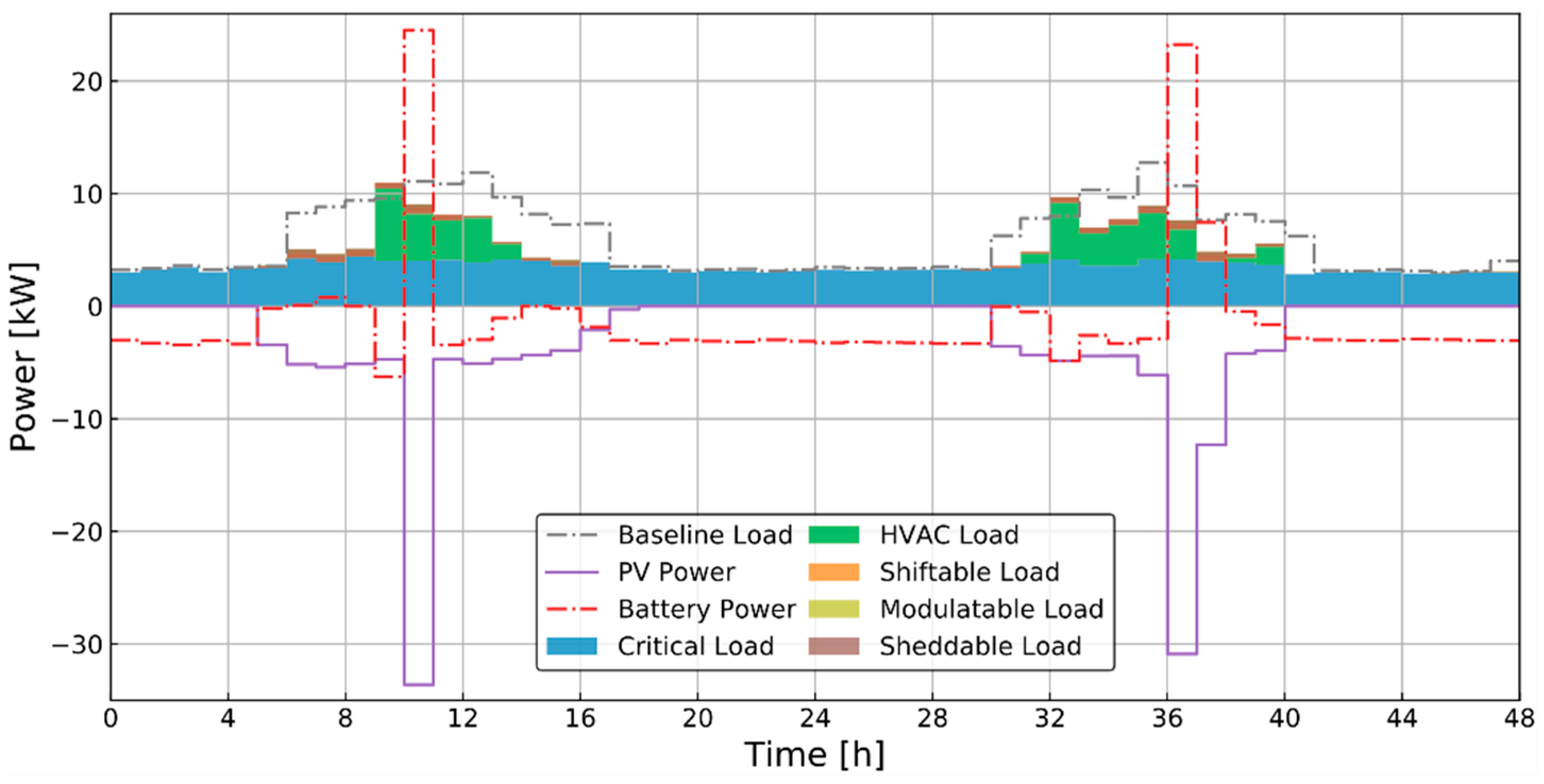
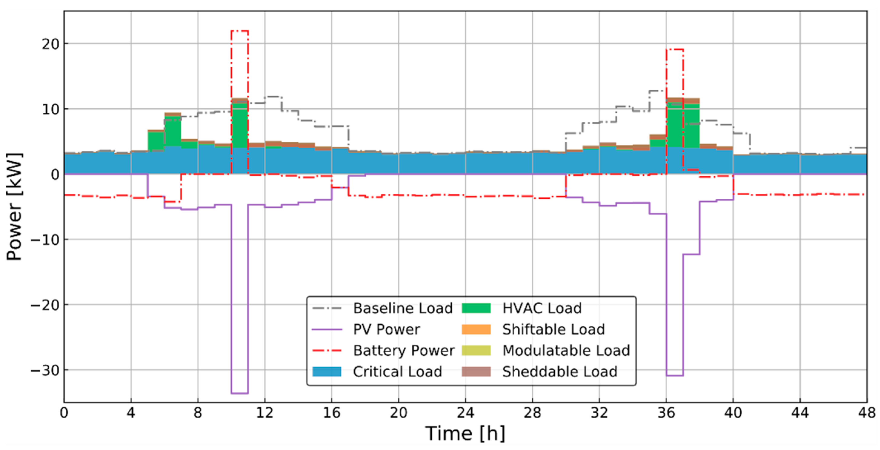
Figure 15 plots the results of the residential building with equal weighting and the objective is to maximize thermal comfort. Compared with Figure 6, we see that when the objective switches from minimizing unserved load to maximizing comfort, there is an obvious increase of HVAC power and the temperature gets closer to the temperature setpoint of 24 $°\mathrm{C}$ (Figure 8). When comparing Figure 16 with Figure 7, we see a decrease of HVAC power usage because before (S21 in Figure 8), the indoor temperature was below 24 $°\mathrm{C}$; when the objective is to minimize the temperature deviation from 24 $°\mathrm{C}$, the required cooling power is actually less. The HVAC power is saved to get the indoor temperature closer to the temperature setpoint.

Comparing Figure 17 with Figure 9, we see a decrease of serving in sheddable load when the objective switches from minimizing unserved load to maximizing comfort. As a result, 63.72% of sheddable load is unserved in this scenario (Table A1). However, the HVAC power also decreases in order to increase the indoor temperature to the temperature setpoint. The saved PV power is charged into the battery as we see an increase of battery charging in Figure 17. Similar observation can be found if we compare Figure 18 with Figure 12, where unserved ratio of sheddable load increases to 99.03% and modulatable to 68.89% due to the change of objective function (Table A1).

To further quantify the impact of weighting factor and objective function, we summarized the community overall KPIs in

Table 6. Community overall PV curtailment and unserved load ratio of each scenario.

Scenario	PV Curtailment Ratio	Unserved Load Ratio
		Sheddable	Shiftable	Modulatable	Critical	Overall
S11	0.00%	0.00%	10.94%	0.00%	0.00%	0.27%
S21_R	8.31%	0.00%	10.94%	0.00%	0.00%	0.27%
S21_I	0.00%	0.00%	10.94%	0.00%	0.00%	0.27%
S21_B	0.00%	0.00%	10.94%	0.00%	0.00%	0.27%
S31	1.03%	0.00%	10.94%	0.00%	0.00%	0.27%
S12	0.00%	64.14%	10.94%	68.89%	0.00%	9.25%
S22_R	13.18%	65.06%	10.94%	77.00%	0.00%	9.54%
S22_I	0.00%	64.13%	10.94%	72.83%	0.00%	9.34%
S22_B	0.00%	64.14%	10.94%	69.23%	0.00%	9.26%
S32	5.43%	65.49%	10.94%	73.64%	0.00%	9.51%

and

Table 7. Community overall room temperature deviation and required battery size of each scenario.

Scenario	$\mathbf{Temperature}\mathbf{Deviation}(°\mathbf{C})$	Battery Size (kWh)
S11	3.04	199.8
S21_R	4.05	215.55
S21_I	2.78	209.64
S21_B	3.10	194.61
S31	3.48	182.91
S12	0.53	218.07
S22_R	0.53	242.05
S22_I	0.53	237.91
S22_B	0.53	210.19
S32	0.53	199.52

. The KPIs include PV curtailment ratio, unserved load ratio, temperature deviation from setpoint, and required battery size. The definition of the PV curtailment ratio is the total curtailed PV energy over the generated energy during the simulation horizon. The unserved load ratio is calculated by dividing the total unserved load by the total original load over the simulation horizon. The definition of the temperature deviation from setpoint is adapted from the root mean square deviation (RMSD), which is the root mean of the square of the deviation between the indoor temperature and the temperature setpoint over the 48-h simulation denoted by:

$$RMSD=\sqrt{\frac{{{\displaystyle \sum }}_{t=1}^H{\left(T_{room}^t-\frac{{\underset{\_}{T}}_{room}+{\overline{T}}_{room}}{2}\right)}^2}{N}},$$

(50)

where $N=48$ is the simulation horizon. Here, the temperature setpoint is selected to be the middle of the comfort temperature range: 24 $°\mathrm{C}$. Lastly, the required battery size is obtained by subtracting the minimum battery SOC from the maximum value. This gives us a sense of how much of the battery capacity has been utilized under different scenarios. Further, this could help to guide the battery sizing to enhance community resilience.

From Table 6, we see that PV curtailment only happens when the residential building is prioritized (S21_R and S22_R) or when occupancy-based weighting is implemented (S31 and S32). This is because the residential building has a relatively small power demand compared to the other two commercial buildings. When it is prioritized by the operator layer, more PV generation is allocated than needed, resulting in PV curtailment. This also echoes our discussions above that allocating purely based on building occupancy status could lead to unfair allocation situations. In the table, the shiftable load unserved load ratio is the same for all scenarios. This is because of our assumption that each shiftable load operates once and only once every day. However, in the original data, some loads might have operated more than once, causing “unserved load” for shiftable loads. Given this, we can consider that all loads are satisfied for the scenarios to minimize unserved load (S11 to S31 in Table 6). When looking at scenarios S12–S32 in Table 6, we see an increase of unserved load as the objective switches to maximizing comfort. The largest unserved load ratio appears in the scenario where residential building is prioritized. From Table 6, the scenarios that perform the best would be S11, S21_I, and S21_B if we only consider PV curtailment and unserved load ratio. In these scenarios, the PV allocation is either equally weighting all buildings or prioritizing those with larger power demand while minimizing the unserved load ratio.

Next, we analyze the temperature deviation and necessary battery size shown in Table 7. We see that all scenarios with the thermal comfort objective experience the fewest temperature deviations. This means that the indoor temperature is well controlled to stay near the temperature setpoint. In the remaining scenarios with the unserved load objective, large deviations in temperature can be seen. For many scenarios, this is due to lower indoor temperatures than the temperature setpoint. Hence, setting the temperature setpoint appropriately can save HVAC energy. However, in our case, the saved energy was either curtailed or charged into the battery instead of satisfying the other loads. This also leads to larger battery sizes in scenarios to maximize comfort (average size: 221.5 kWh) than scenarios to minimize unserved load (average size: 200.5 kWh). Therefore, a co-optimization of thermal comfort and unserved load is necessary with the benefit of less curtailment, smaller unserved load ratio, assured thermal comfort, as well as smaller battery size.

The above simulation results highlight the impact of the objective function on KPI outcomes. From the above discussions, we identified that if only PV curtailment and unserved load ratio are considered, the best option is to allocate the PV resource either equally weighting or prioritizing buildings with larger power demand while minimizing unserved load ratio. After further looking at other indices, we noticed that choosing the optimization objective to track an appropriately selected indoor room temperature setpoint will save HVAC energy. However, this will not lead to lower unserved ratio for other load types. Instead, the PV curtailment could increase. The two objectives have a competitive relationship: serving more HVAC power to increase thermal comfort will decrease the other served load.

5. Conclusions

We proposed a novel decentralized control architecture for renewable resource allocation and load scheduling of resilient communities. This MPC-based optimization architecture consists of a community operator layer that allocates the daily PV power generation to achieve the community-wide optimum and a building agent layer that schedules building loads to achieve its local optimum in each building. Three allocation methods were tested for the operator layer: equally weighted, weighted based on building priority, and weighted based on building occupancy. At the building level, two objective functions were compared: minimizing unserved load ratio versus maximizing thermal comfort. The proposed framework has the advantage of distributed computational effort and is easier to be scaled up than traditional centralized control, which is not robust for large-scale deployment. Additionally, the comparison between different combinations of allocation methods and objective functions provides guidance for real-world deployment by community and microgrid operators.

Through a case study for an islanded community in FL for 48 h, we evaluated the proposed architecture with respect to user-centric performance metrics (KPIs). We found that the allocation process is mostly constrained by the building load flexibility. More specifically, buildings with less load flexibility (i.e., ice cream shop with large critical loads) tend to be allocated more PV generation than other buildings. Additionally, when prioritizing buildings according to occupancy status, the building with longer occupancy duration is allocated more PV power, which may not result in a fair allocation method and could lead to more PV curtailment.

Additionally, through the analysis of different objective functions, we found that setting the objective to target at an appropriately selected indoor temperature setpoint will result in increased HVAC energy savings. However, in our case study this did not lead to lower unserved ratio for other load types. Instead, the PV curtailment increased. The two objectives have a competitive relationship: serving more HVAC power to increase thermal comfort will decrease the other served load. Therefore, it is necessary for the building agent to have multi-objective optimization to minimize unserved load ratio and maximize comfort simultaneously. This will bring the benefit of less curtailment, smaller unserved load ratio, assured thermal comfort, as well as smaller battery size. However, the weighting between the two objectives needs to be carefully selected as their scales are quite different.

For future work, we will conduct multi-objective optimization for the building agent layer to investigate the trade-off between minimizing unserved load ratio and maximizing thermal comfort. Uncertainty of PV generation should also be included to reflect the impact of different weather conditions.