Optimization of a 660 MW_e Supercritical Power Plant Performance—A Case of Industry 4.0 in the Data-Driven Operational Management. Part 2. Power Generation

Abstract

Modern data analytics techniques and computationally inexpensive software tools are fueling the commercial applications of data-driven decision making and process optimization strategies for complex industrial operations. In this paper, modern and reliable process modeling techniques, i.e., multiple linear regression (MLR), artificial neural network (ANN), and least square support vector machine (LSSVM), are employed and comprehensively compared as reliable and robust process models for the generator power of a 660 MW_e supercritical coal combustion power plant. Based on the external validation test conducted by the unseen operation data, LSSVM has outperformed the MLR and ANN models to predict the power plant’s generator power. Later, the LSSVM model is used for the failure mode recovery and a very successful operation control excellence tool. Moreover, by adjusting the thermo-electric operating parameters, the generator power on an average is increased by 1.74%, 1.80%, and 1.0 at 50% generation capacity, 75% generation capacity, and 100% generation capacity of the power plant, respectively. The process modeling based on process data and data-driven process optimization strategy building for improved process control is an actual realization of industry 4.0 in the industrial applications.

1. Introduction

Given the increased domestic and commercial industrial sectors, almost 100% of energy consumption has increased over the last four decades [1]. Harvesting the rising energy demand through the inefficient power complexes and their poor operation control, not only the operation cost of power generation is increased significantly, but huge volumes of greenhouse gas emissions also cause degradation and deterioration of the environment. Over the past few decades, researchers and energy experts are closely collaborating in a wide range of research activities to mitigate the harmful impacts of power generation to ensure sustainable power generation and environmental protection. [2,3,4,5,6,7,8,9,10,11,12,13,14,15,16].

The power generation from large commercial power plants is a highly complex and critical industrial operation. A large number of thermo-electric operating parameters are simultaneously controlled and monitored via distributed control systems. The large volume of operation data and the underlying nonlinear interactions analysis in the operating parameters make it practically impossible by conventional analytical means.

The advanced and sophisticated artificial intelligence (AI) algorithms are designed to analyze the high-dimensional featured data describing complex industrial operations [17,18,19]. With the development of information and communication technologies (ICT), the collection, storage, and retrieval of a process’s large volume of operation data are significantly improved. Modern data analytics techniques and computationally inexpensive software tools are fueling the commercial applications of data-driven decision making and process optimization strategies for complex industrial operations [20]. Machine learning and deep learning, the reliable and promising data analytics domains of AI, are practically suitable for modeling, controlling, and optimizing the processes. However, the comprehensive analysis of the optimization and operation management of power generation systems conducted in the true spirit of industry 4.0 is scarcely reported in the literature [20].

A comprehensive review of AI applications’ current status in the energy systems is presented in the literature. The key challenges impeding AI inclusion in real-life applications are extensively explored, and the widespread AI-based applications in the various industrial sectors are predicted [21,22]. A preliminary study is carried out to develop a platform built in the context of industry 4.0. Deep learning models employed to model the waste to heat recovery system have performed well in mapping the system’s dynamic response [20]. LSSVM based hybrid models are reported for forecasting the energy demand of the grid [23] and the energy consumption of complex industrial processes to ensure the efficient operation management and control of the cement industry [24].

Elfaki et al. have modeled the electrical output power of a combined cycle power plant by ANN using four input variables. The deviation between the target value and validation dataset value is negligible, signifying the model’s effectiveness [25]. Zhu, H., et al. have employed wavelet decomposition and ANN to forecast power generation from the photovoltaic power plant. The developed methodology presents better performance and forecasting precision as compared to traditional ANN models [26]. The researchers have reported the modeling of wind turbine generator operation by ANN and LSSVM techniques under various operating parameters [27,28,29]. However, the literature concerning the generator power modeling of a large-scale power complex under various operating scenarios is scarce.

In this paper, various process modeling techniques, i.e., MLR, ANN, and LSSVM, are utilized and comprehensively compared for the operational analysis of the generator power production from a 660 MW_e supercritical coal power plant. Considering 330 MW_e and 660 MW_e as 50% and 100% unit load (that is essentially the resistive power, and power factor between 0.85 to 1.00), the generator power (that accounts for both resistive and reactive power production from the power plant), is varied from 355 MVA to 715 MVA (50% generation capacity to nearly 100% generation capacity). The power plant’s characteristics operation data under the various power generation scenarios are taken from the Supervisory Information System (SIS). After machine learning techniques perform the data visualization test, i.e., self-organizing feature map (SOFM), MLR, ANN, and LSSVM, are employed to predict the generator’s power. The best performing and reliable process model is utilized for two principal objectives, i.e., (1) to plot the characteristics response of the generator power under the failure mode of the power plant; and (2) to optimize the generator power of the supercritical power plant for effective control of thermo-electric operating parameters.

Two AI techniques applications are presented in this study. In the first case, carefully designed computer-simulated Monte-Carlo experiments are performed on the AI process models to develop a standard operating procedure for failure mode recovery and mitigation of cost of failure. Secondly, AI process models are employed as a very successful operation control excellence tool. The paper’s contribution constitutes a further step ahead in the spirit of industry 4.0 data analytics for actual commercial processes in various industrial sectors.

2. Schematic of Power Plant

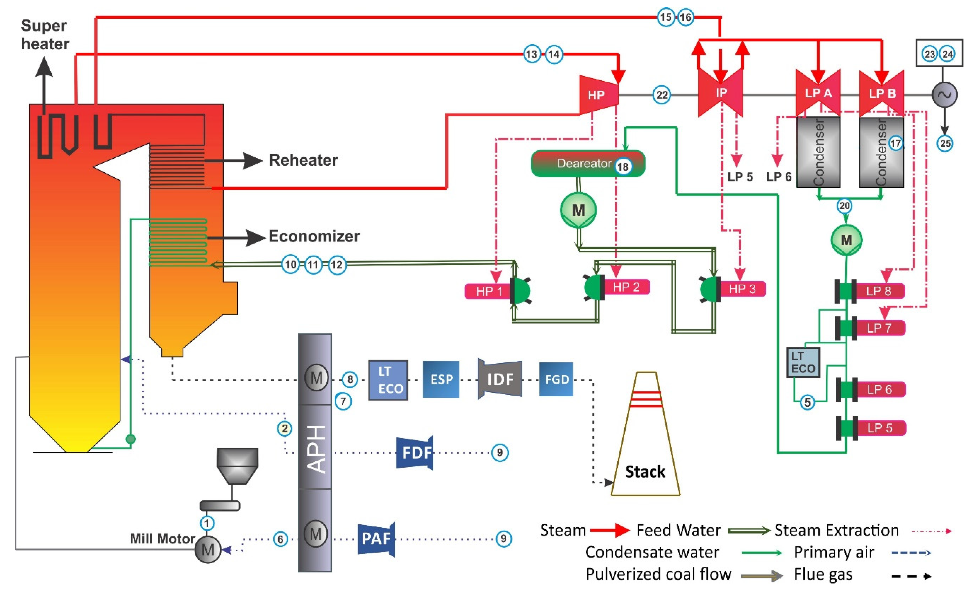
The schematic process flow of the pulverized coal power plant is shown in Figure 1. Two basic systems can be distinguished; one is the flue gas system, and the second is the water and steam system. In the flue gas system, the primary air provided by the primary air fan (PAF) is heated by air pre-heater (APH). The hot primary air is used to transfer the pulverized coal from the coal mill to the boiler burners for coal combustion. After passing through APH, the secondary air provided by the forced draft fan (FDF) is used for the complete combustion of coal in the boiler. The hot gases produced after coal combustion, known as flue gas, transfer the heat to the boiler’s heating surfaces and converts water to supercritical or subcritical steam. The flue gas leaving the boiler heats primary and secondary air through APH. Induced draft fan (IDF) draws out the flue gas from the boiler and maintains negative pressure inside the furnace. The electrostatic precipitator (ESP) and flue gas desulphurization (FGD) system are installed to remove the particulate matter, Hg, and SO_x in the flue gases. After that, clean flue gas is discharged to the atmosphere via stack.

Feed water is an essential part of the steam power plant operation and known as the power plant’s blood. The condensate pump takes condensate water from the condenser’s hot well, pressurizes it, and passes it on to low pressure (LP) heaters (LP8, LP7, LP6, and LP5). A part of feed-water flow taken from the outlet of LP8 and LP7 is diverted to LT-Economizer (LT ECO) for feed water heating by the flue gas exhaust from the boiler, and then is mixed with the feed-water coming out of LP7 and directed to LP6 and LP5 for further heating, and sent to deaerator. In the deaerator, oxygen and other dissolved gases, which can cause rusting and corrosion in the boiler, are removed from the feed water. Feed water pump then pressurizes the feed water to the reacquired pressure. Feed water passes through high pressure (HP) heaters (HP3, HP2, HP1), where the temperature of feed water is increased before entering the boiler’s economizer. In LP and HP heaters, feed water is heated by steam extractions from different stages of turbines. Then, the preheated feed water enters the boiler’s economizer, super-heater, and finally leaves the boiler as the steam of reacquired temperature and pressure. The pressurized steam expands in the HP turbine, where its temperature and pressure is dropped. As steam temperature leaving the HP turbine is low and to avoid condensation of steam in the latter stage of intermediate pressure (IP) turbine, steam is heated in re-heater before entering the IP turbine. The reheat steam expands in the IP turbine and then in LP turbines A and B (LPA and LPB). After expanding in LPA and LPB turbines, steam is condensed, and the cycle continues. The expansion of steam in the turbines helps rotate the turbines, which are mounted on the same shaft, and the shaft is coupled with the generator for the production of electricity.

The sensors are installed at various points for measuring the values of different thermo-electric operating parameters of the power plant. However, soft sensors take the input from the other measuring sensors and record a particular parameter by the specified mathematical operator that cannot be measured directly. The make and model number of the sensors involved in this study are mentioned in

Table 1. Summary of the sensors for various thermo-electric operating parameters of power plant.

	Sensor	Make	Model
1	Coal flow rate (Mc)	Vishay Precision Group (USA)	3410
2	Air flow rate (Ma)	Siemens (Germany)	7MF4433-1BA22-2AB6-Z
3	Water/Coal ratio (w/c)	Soft sensor	Soft sensor
4	Middle temp. (Tmid)	Anhui Tiankang China Thermocouple	WRNR2(K TYPE)
5	LT Eco water outlet temp. (TLT.ECO)	Anhui Tiankang China Thermocouple	WRNR2(K TYPE)
6	APH air outlet temp. (Ta)APH	Anhui Tiankang China Thermocouple	WRNR2(K TYPE)
7	% O2 in flue gas at APH outlet (% O2)	Walsn (Canada)	0AM-800-R
8	Flue gas temp. after APH ((Tfg)APH)	Anhui Tiankang China Thermocouple	WRNR2(K TYPE)
9	Ambient temp. (Tamb)	Anhui Tiankang China Thermocouple	WRNR2(K TYPE)
10	Feed water pressure (FWP)	Siemens (Germany)	7MF4033-1GA50-2AB6-Z
11	Feed water temp. (FWT)	Anhui Tiankang China Thermocouple	WRNR2(K TYPE)
12	Feed water flow (FWF)	Siemens (Germany)	7MF4533-1FA32-2AB6-Z
13	Main steam pressure (MSP)	Siemens (Germany)	7MF4033-1GA50-2AB6-Z
14	Main steam temp. (MST)	Anhui Tiankang China Thermocouple	WRNR2(K TYPE)
15	Reheat pressure (RHP)	Siemens (Germany)	7MF4033-1GA50-2AB6-Z
16	Reheat temp. (RHT)	Anhui Tiankang China Thermocouple	WRNR2(K TYPE)
17	Absolute condenser vacuum (Pvac)	Siemens STTRANS D PS III	7MF4233-1GA50-2AB6-Z
18	Deaerator temp. (Td)	Anhui Tiankang China Thermocouple	WRNR2(K TYPE)
19	Attemperation water flow rate(AWF)	Siemens (Germany)	7MF4533-1FA32-2AB6-Z
20	Condensate temp. (TC)	Anhui Tiankang China Thermocouple	WRNR2(K TYPE)
21	Auxiliary power (Paux)	Nanjing Suatak Measurement and Control System	STM3-WT-3-155A4BN
22	Turbine speed (N)	Braun (Germany)	A5S
23	Excitation voltage (Exc. V)	Siemens (Germany)	SPPA-E3000 SES 530
24	Excitation current (Exc. I)	Siemens (Germany)	SPPA-E3000 SES 530
25	Generator power (G.P)	Nanjing Suatak Measurement and Control System	STM3-WT-3-555A4BY

.

3. Training Data and Data Visualization

3.1. Training Data for Process Modeling

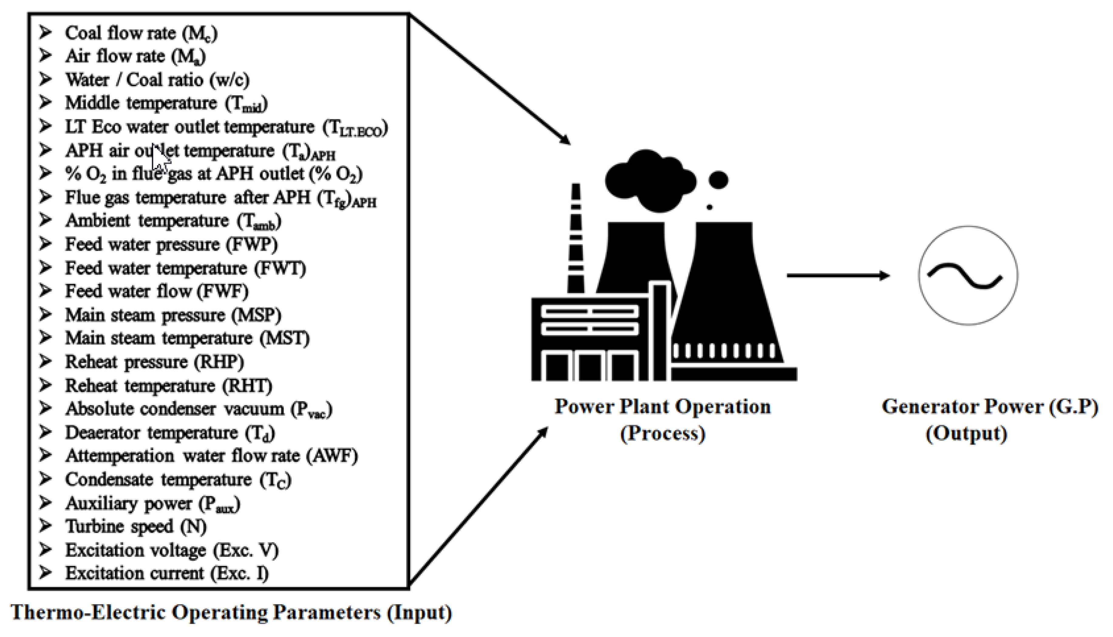
In this paper, twenty-four thermo-electric operating parameters of the power plant are taken to model the generator power under various power generation scenarios. The thermo-electric operating parameters are selected based on the operation engineers’ experience and the comprehensive literature review [30,31,32,33,34,35]. The operating parameters are taken from the boiler, turbine, and generator sides of the power plant and are critically controlled within the operating ranges. The average values of the coal used at the power plant are listed in

Table 2. Properties of coal (air-dried basis).

LHV MJ/kg	Properties of Coal/wt.%
24.23	Moisture	Volatile Mater	Ash	Sulfur	Fixed Carbon by diff.
	2.5	23.73	16.6	0.55	57.66

.

Moreover, the input-process-output diagram connecting the thermo-electric operating parameters of the power plant (input variables) and generator power (output) is shown in Figure 2.

The power plant’s operation data representing the detailed and extensive information on power generation under the influence of selected thermo-electric operating parameters are taken from the SIS portal. The total 1900 data points of the thermo-electric operating parameters under the power plant’s continuous power generation mode are retrieved to model complex and nonlinear power generation operations. The list of the thermo-electric operating parameters with the measuring units, minimum-maximum operating range, and standard deviation is mentioned in

Table 3. Statistics of the training data.

Parameters	Unit	Min	Max	St. Dev
Coal flow rate (Mc)	t/h	129	252	86.76
Air flow rate (Ma)	t/h	1469	2636	825
Water/Coal ratio (w/c)	-	6.98	8.49	1.07
Middle temp. (Tmid)	°C	343	425	57.78
LT Eco water outlet temp. (TLT.ECO)	°C	90	100	6.94
APH air outlet temp. (Ta)APH	°C	311	352	29.43
% O2 in flue gas at APH outlet (% O2)	%	5.27	8.50	2.28
Flue gas temp. after APH (Tfg)APH	°C	120	157	26.84
Ambient temp. (Tamb)	°C	5.0	43.0	27.2
Feed water pressure (FWP)	MPa	15.0	30.0	10.39
Feed water temp. (FWT)	°C	260	299	27.67
Feed water flow (FWF)	t/h	942	1987	738.98
Main steam pressure (MSP)	MPa	13.0	24.4	8.05
Main steam temp. (MST)	°C	550	569	13.97
Reheat pressure (RHP)	MPa	2.6	5.0	1.69
Reheat temp. (RHT)	°C	553	569	10.88
Absolute Condenser vacuum (Pvac)	kPa	95.60	89.30	4.48
Deaerator temp. (Td)	°C	164	190	18.59
Attemperation water flow rate (AWF)	t/h	4	97	65.94
Condensate temp. (TC)	°C	27	47	13.8
Auxiliary power (Paux)	MWe	20.3	29.2	6.31
Turbine speed (N)	Rpm	2986	3017	22.49
Excitation voltage (Exc. V)	V	186	435	182.65
Excitation current (Exc. I)	A	1940	4144	1629.85
Generator power (G.P)	MVA	355.1	714.9	254.44

.

3.2. Self-Organizing Feature Map (SOFM)

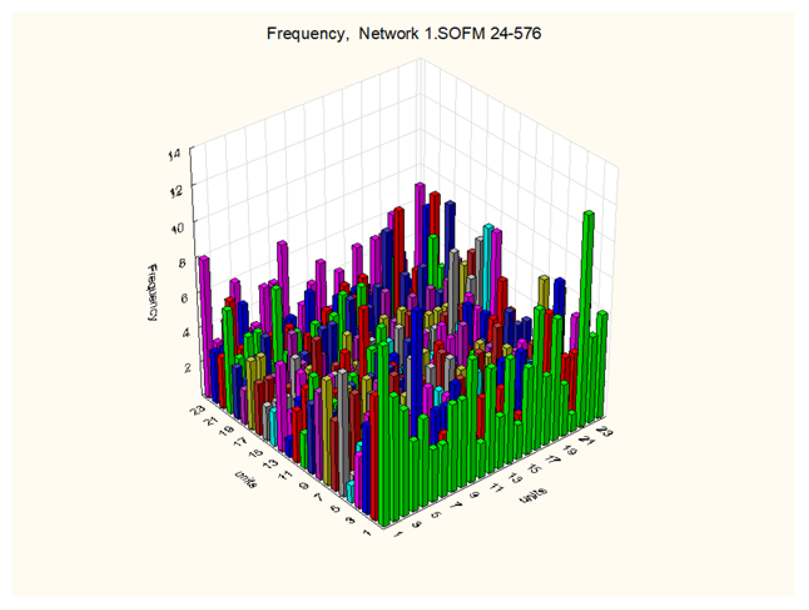
To confirm the presence of useful and featured information that may exist in the power generation’s characteristics operation data, a reliable and sophisticated machine learning data visualization technique, i.e., self-organizing feature map (SOFM), is used [36]. SOFM is an unsupervised learning machine that maps the underlying possible statistical features of the high-dimensional input space data on the nodes of a two-dimensional square lattice. The square lattice’s length is equal to the input space dimensions [2,36]. SOFM has an excellent ability to distribute the input space data on the nodes in homogenous groups and is used in many real-life applications [37,38,39]. In this work, a two-dimensional square lattice carrying 24 × 24 nodes is created, and the distribution of the thermo-electric operating parameters data, which are the input space data, is shown in Figure 3. The z-axis represents the frequency of occurrence of data points on a node. It is evident from Figure 3, that the data points are reasonably well-distributed. Therefore, the SOFM directs to construct the process models of generator power using the retrieved data of the power plant’s thermo-electric operating parameters.

4. The Theoretical Background of Modeling Techniques

An essential theoretical background of the three modeling techniques used in this study is provided below.

4.1. Multiple Linear Regression

Multiple linear regression (MLR) is a statistical model which describes how various inputs affect the output of a function. It is an extension of simple linear regression and incorporates two or more independent variables to model the dependent variable. The model works to create a relationship between a few or more input variables and an output variable by fitting a linear mathematical equation to the observed data. MLR is a computationally downscaling technique that is widely used in statistical analysis [40].

Each value of the independent variable x is associated with a value of the dependent variable y, and if y is a dependent variable and x₁, x₂, …, x_i are independent variables, then the basic MLR model will be given in the following equation,

$$y= b_0+ b_1{x}_1+ b_2{x}_2 + \dots +b_i{x}_i + e$$

(1)

where b₀, b₁, b₂,…, b_i are the regression coefficients, and “e” accounts for the error in fitting the regression line across the observed data [41].

4.2. Artificial Neural Network

Artificial neural network-based algorithms are inspired by the working of the human brain and are capable to effectively dig and learn the relationships among the complex, nonlinear, and multi-dimensional set of variables [32].

A typical ANN consists of three layers: an input layer, a hidden layer, and an output layer. The number of neurons in the input layer is equal to the number of input variables. After multiplying by the weights with the input variables data, the information is fed to the hidden layer. A transfer function is applied at the hidden layer to process the received information. The information from the hidden layer is multiplied by a weight and is transferred to the output layer. The output layer contains neurons with a transfer function to process the previous layer’s values and yields a final output value [42].

An ANN model is described mathematically with the following equation,

$$y_i=f_2\left({\displaystyle \sum }_i^n{W}_2\left[f_1\left({\displaystyle \sum }_i^n{x}_i\ast W_1+b_1\right)\right]+b_2\right)$$

(2)

where, $x$ and $y$ are the input and output variables and, i =1,2,3,…, n equal to the number of data points of input and output variables. W₁ and W₂ are the weights at the input and hidden layer, b₁ and b₂ are the biases at different layers and f₁ and f₂ are the transfer functions in the hidden and output layer, respectively.

The output value calculated by ANN is compared with the output variable’s actual value, and error is calculated. If the error is higher than the threshold value, the weights and biases at the layers are modified, and calculations are performed in each iterative cycle unless the error lies within the acceptable level [43].

4.3. Least Square Support Vector Machine

Least square support vector machine training algorithms are among the efficient supervised learning techniques used for their good generalization ability and accuracy. LSSVM training is based on the structural risk minimization principle (SRM), and its basic concept is to transform the data into a high-dimensional feature space and solve the nonlinear problems in a linear pattern [42]. LSSVM uses squared errors as the cost function and can be written as an optimization problem with equal constraints [42],

$$\underset{\mathit{w},b,\mathit{\xi }}{min}J\left(\mathit{w},\mathit{\xi }\right)=\frac{1}{2}{\mathit{w}}^{\mathrm{T}}\mathit{w}+\frac{1}{2}\gamma {\displaystyle \sum }_{i=1}^n {\xi }_i^2$$

(3)

$$such that: y_i={\mathit{w}}^{\mathrm{T}}\phi \left({\mathit{x}}_i\right)+b+{\xi }_i,i=1,\cdots ,n$$

(4)

where w is a weight vector, $\gamma$ is a penalty parameter, $\xi$ is the ith error variable, $\phi$ is a nonlinear function mapping inputs from the data to a higher feature space, and b is a bias.

According to the Karush-Kuhn-Tucker (KKT) theory, the solution can be obtained by solving a linear equation in terms of the dual variables, and then the LSSVM model is given as follows [42],

$$y\left(\mathit{x}\right)={\displaystyle \sum }_{i=1}^n {\alpha }_{i}K\left(\mathit{x},{\mathit{x}}_i\right)+b$$

(5)

where ${\alpha }_i$ is a KKT multiplier, and K(.,.) is a radial basis function that simplifies the mapping process. The kernel function is linear, gaussian, and polynomial type, and generally, the gaussian kernel function is used in the development of LSSVM models for mapping the complex and nonlinear interactions among the data. Gaussian kernel function can be expressed as:

$$K\left(x,x_j\right)=\exp \left(-\parallel x-x_j{\parallel }^2\right).$$

(6)

More detailed information on the LSSVM model development can be found elsewhere [44].

5. Development of Process Models

The least-square approach is used for developing the MLR model. The deviation between the actual and observed values of the process is computed, termed as residuals. In the least-square model approach for the best-fit line, the sum of the square of residuals is minimized. The residuals are normally distributed, having a mean equal to zero and standard deviation (ϭ).

The ANN model is a multi-layered perceptron (MLP) that consists of three layers, an input layer, a hidden layer, and an output layer [45]. The hidden layer itself may consist of one or more layers. It is proved that one hidden layer is enough to approximate the nonlinearity present in the data provided enough number of neurons are present in the hidden layer [46]. The optimum number of neurons in the hidden layer is determined by hit and trial methods [47,48]. The feedforward backpropagation network algorithm is used in this work. Gradient descent with momentum is employed as a training function, tangent hyperbolic and purelin is employed as transfer functions at the hidden and output layer of MLP, respectively [2,44]. ANN training is carried out until one of the two stopping criteria is met, i.e., either a 0.0000001 change in convergence error or a maximum number of epochs is reached [2,49]. In this work, multiple ANNs are trained, and the number of neurons in the hidden layer is varied from 10 to 36 to find the optimal number of hidden layer neurons based on the validation test, as mentioned in the Section 5.2.

LSSVM can be trained quite effectively for modeling a system based on the structural risk minimization (SRM) principle. A Gaussian kernel function is generally used for mapping the complicated nonlinear relationship between the input and output variables onto the feature space [42]. It is essential to mention here that the training data set should be standardized for developing a useful LSSVM model. Bayesian optimizer and expected improvement per second plus acquisition function is used to optimize $\gamma$ for LSSVM under 30 epochs [50,51,52,53].

The input and output data described in Table 3 are used to develop models. The 24 data values from the top 24 rows of Table 3 and one from the last row of Table 3 correspond to input and output parameters.

5.1. Errors and Evaluation Criteria

The developed process models’ performance is evaluated based on the model’s prediction error against the validation dataset unseen to the development phase models. Coefficient of determination (R²), root-mean-square error (RMSE), normalized RMSE (NRMSE), mean absolute error (MAE), and mean absolute percentage error (MAPE) of the models’ prediction are calculated to evaluate the robustness and effectiveness of the process models. The definition of the evaluation criteria is given below,

$$R^2=1-\frac{{{\displaystyle \sum }}_{i=1}^n{\left(y_i-{\widehat{y}}_i\right)}^2}{{{\displaystyle \sum }}_{i=1}^n{\left(y_i-{\overline{y}}_i\right)}^2}$$

(7)

$$RMSE=\sqrt{\frac{1}{n}{\displaystyle \sum }_{i=1}^n{\left(y_i-{\widehat{y}}_i\right)}^2 }$$

(8)

$$NRMSE= \frac{RMSE}{y_{max-} y_{min}}\ast 100\%$$

(9)

$$MAE=\frac{1}{n}{\displaystyle \sum }_{i=1}^n \left|y_i-{\widehat{y}}_i\right|$$

(10)

$$MAPE=\frac{1}{n}{\displaystyle \sum }_{i=1}^n{\left|\frac{y_i-{\widehat{y}}_i}{y_i}\right|}^{″}\ast 100\%$$

(11)

where, n is the sample size, ${\widehat{y}}_i$, $y_i$ and ${\overline{y}}_i$ are the predicted values, actual values, and mean of actual values; $y_{max}$ and $y_{min}$ are the maximum and minimum value of $y_i,$ respectively.

5.2. Validation Case against Unseen Data

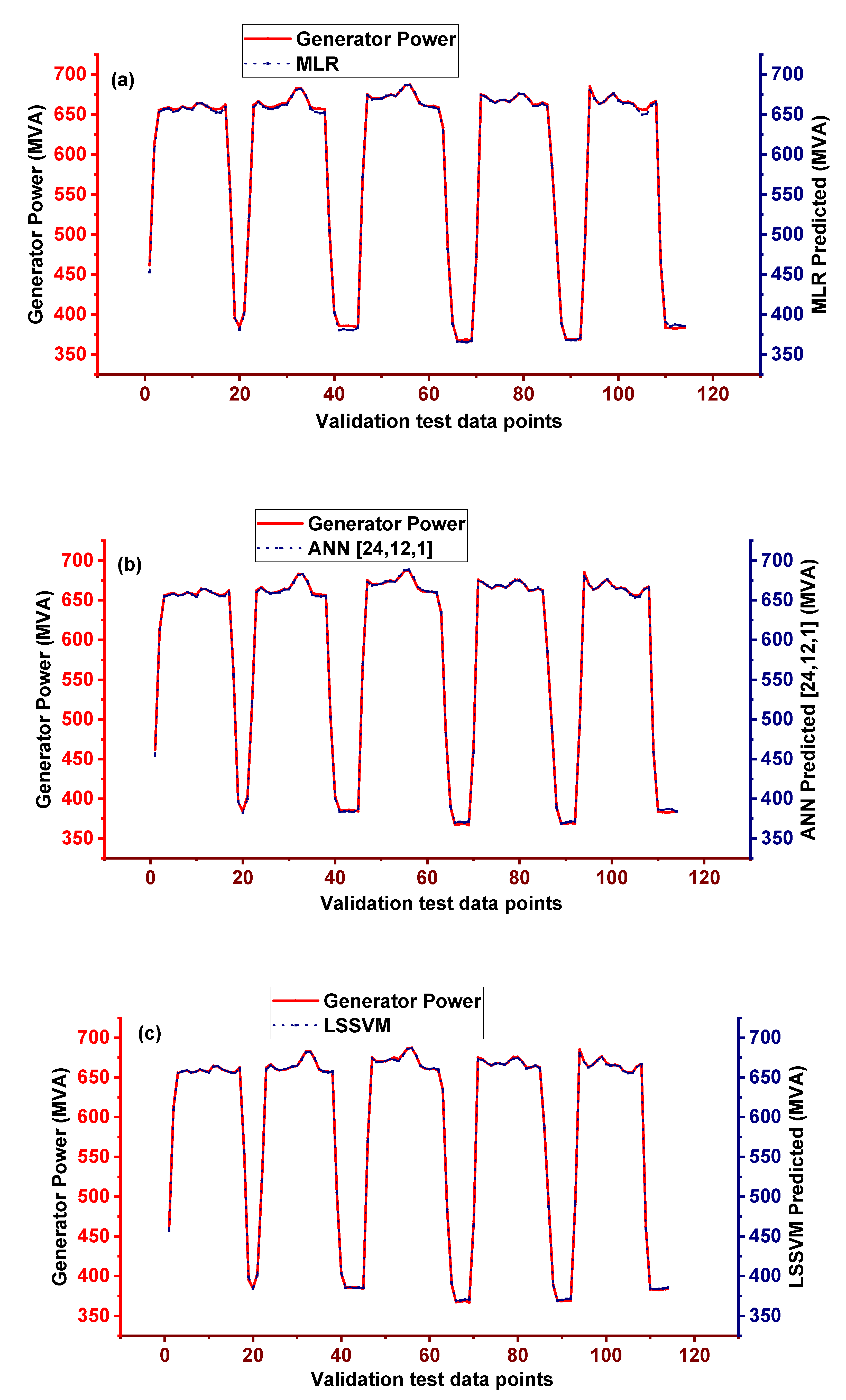
After the training of MLR, ANN, and LSSVM process models, all models are validated against unseen generator power data that was not added in the training dataset during the models’ development. The unseen data consist of 110 data points of the thermo-electric operating parameters and entail the extensive and diverse operating state of power plant operation.

The validation performance of the developed MLR model is evaluated based on the evaluation criteria. R², RMSE, NRMSE, MAE and MAPE for MLR model are 0.99958, 2.674 MVA 0.834%, 1.940 MVA, and 0.007%, respectively.

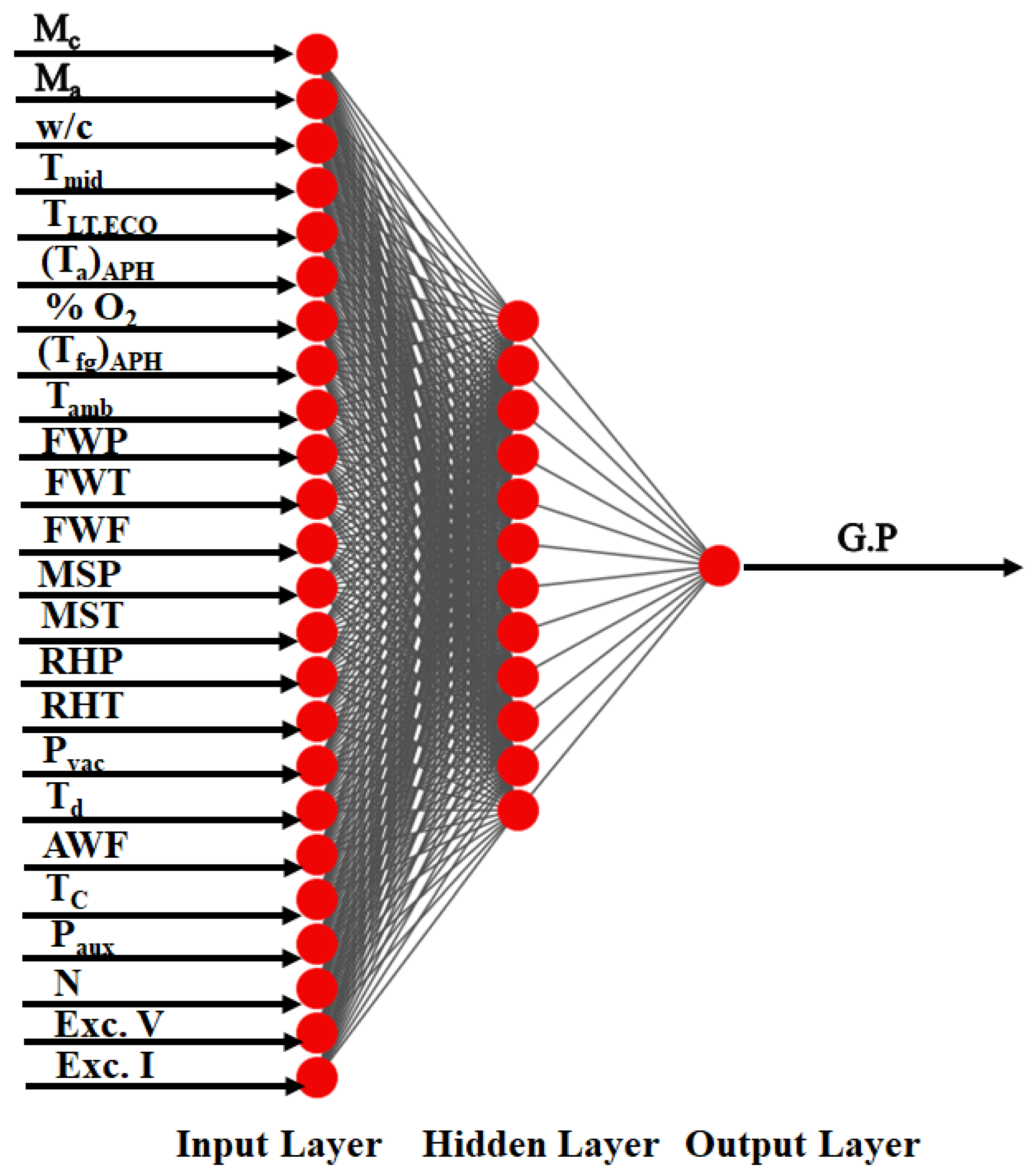
Multiple ANN models are trained based upon the number of hidden layer neurons varied from 10 to 36. Each of the trained ANN models’ performance is evaluated against the validation data set and presented in

Table 4. Performance evaluation of ANNs against validation dataset.

Hidden Layer Neurons	R2	RMSE	NRMSE	MAE	MAPE
-	-	MVA	%	MVA	%
10	0.999369	3.177	0.991	2.171	0.009
11	0.999685	2.344	0.731	1.597	0.006
12	0.999707	2.093	0.653	1.447	0.006
13	0.999218	3.391	1.057	2.173	0.009
14	0.999267	3.638	1.134	2.528	0.01
15	0.999612	2.609	0.813	1.903	0.007
16	0.999692	2.212	0.69	1.534	0.006
17	0.999468	3.095	0.965	2.177	0.008
18	0.999395	3.084	0.962	2.123	0.008
19	0.999536	2.401	0.749	1.672	0.007
20	0.999568	2.532	0.79	1.98	0.007
21	0.999684	2.218	0.692	1.627	0.006
22	0.999447	2.899	0.904	2.037	0.008
23	0.999491	2.742	0.855	2.055	0.008
24	0.999655	2.447	0.763	1.853	0.007
25	0.999244	3.281	1.023	2.228	0.009
26	0.999551	2.552	0.796	1.81	0.007
27	0.999656	2.608	0.813	1.931	0.007
28	0.999601	2.549	0.795	1.669	0.007
29	0.999337	3.595	1.121	2.677	0.01
30	0.999438	3.066	0.956	2.164	0.008
31	0.999698	2.328	0.726	1.831	0.006
32	0.999556	2.533	0.79	1.783	0.007
33	0.999495	2.931	0.914	2.132	0.008
34	0.99924	3.354	1.046	2.729	0.009
35	0.999483	2.817	0.878	2.065	0.008
36	0.999668	2.27	0.708	1.723	0.006

. By comparing the performance of trained ANN models, the ANN model having twelve number of neurons in the hidden layer has outperformed the remaining ANN models in terms of the evaluation criteria for assessing the performance of models and is represented as ANN [24-12-1]. The structure of the ANN [24-12-1] is shown in Figure 4. The R², RMSE, NRMSE, MAE and MAPE for ANN [24-12-1] are 0.999707, 2.093 MVA, 0.653%, 1.447 MVA and 0.006% respectively.

Similarly, the performance of the LSSVM model is also measured based on the evaluation criteria. R², RMSE, NRMSE. MAE and MAPE for the LSSVM model are 0.999878, 1.521MVA. 0.474%, 1.069 MVA, and 0.004%, respectively. The comparative performance analysis of MLR, ANN [24-12-1], and LSSVM model performance against the evaluation criteria are presented in Figure 5 and

Table 5. Performance comparison of MLR, ANN, and LSSVM models.

Models	R2	RMSE	NRMSE	MAE	MAPE
	-	MVA	%	MVA	%
MLR	0.99958	2.674	0.834	1.940	0.007
ANN [24-12-1]	0.999707	2.093	0.653	1.447	0.006
LSSVM	0.999858	1.521	0.474	1.069	0.004

.

According to Table 5, the LSSVM model has relatively higher superiority over the MLR and ANN models in predicting the plant’s generator power. Therefore, the LSSVM model is selected for further analysis of interest, as discussed in the next sections.

6. Results and Discussion

The successfully validated LSSVM model is used to predict the power plant’s generator power for various operating strategies of the power plant. The approach provides insight into the influence of power plant thermo-electric operating parameters on power generation. The minimum, average, and maximum values of the thermo-electric operating parameters at 50% and 100% unit load are listed in

Table 6. Statistics of thermo-electric operation parameters at 50% and 100% unit load.

Operating Parameters		50% Unit Load (MWe)			100% Unit Load (MWe)
	Unit	Min	Avg	Max	Min	Avg	Max
Coal flow rate (Mc)	t/h	129	137	156	210	238	252
Air flow rate (Ma)	t/h	1469	1559	1703	2197	2472	2636
Water/Coal ratio (w/c)	-	6.98	7.52	8.08	7.63	8.09	8.49
Middle temp. (Tmid)	°C	343	356	377	410	417	425
LT Eco water outlet temp. (TLT.ECO)	°C	94	98	100	90	93	100
APH air outlet temp. (Ta)APH	°C	311	318	334	332	343	352
% O2 in flue gas at APH outlet (% O2)	%	7.37	7.93	8.50	5.27	5.88	6.85
Flue gas temp. after APH (Tfg)APH	°C	120	127	144	129	137	157
Ambient temp. (Tamb)	°C	5.1	25.2	39.3	5.0	25.7	43.3
Feed water pressure (FWP)	MPa	15.4	16.2	18.0	26.8	29.7	30.0
Feed water temp. (FWT)	°C	260	263	268	291	298	299
Feed water flow (FWF)	t/h	942	1032	1139	1676	1923	1987
Main steam pressure (MSP)	MPa	13.0	13.7	15.3	22.1	24.1	24.4
Main steam temp. (MST)	°C	550	567	569	552	567	569
Reheat pressure (RHP)	MPa	2.6	2.8	3.5	3.4	4.8	5.0
Reheat temp. (RHT)	°C	553	567	569	561	567	568
Absolute condenser vacuum (Pvac)	kPa	95.60	94.10	91.90	95.50	93.60	89.40
Deaerator temp. (Td)	°C	164	166	170	181	187	190
Attemperation water flow rate (AWF)	t/h	5	39	81	6	58	97
Condensate temp. (TC)	°C	27	33	40	31	35	47
Auxiliary power (Paux)	MWe	20.3	22.2	24.0	25.4	27.8	29.2
Turbine speed (N)	Rpm	2986	3003	3017	2986	3002	3017
Excitation voltage (Exc. V)	V	186	218	277	297	359	431
Excitation current (Exc. I)	A	1940	2259	2845	3022	3556	4124

. Comprehensive Monte-Carlo experiments are constructed, and gaussian noise is equal to one percent of the operating range of the thermo-electric operating parameters [54,55]. It is essential to mention here that the generator power trends are constructed with a 99% confidence interval to ensure the relationship and interaction among the thermo-electric operating parameters and generator power, as discussed in the next sections.

6.1. The Combined Effect of Excitation Voltage and Excitation Current on the Generator Power

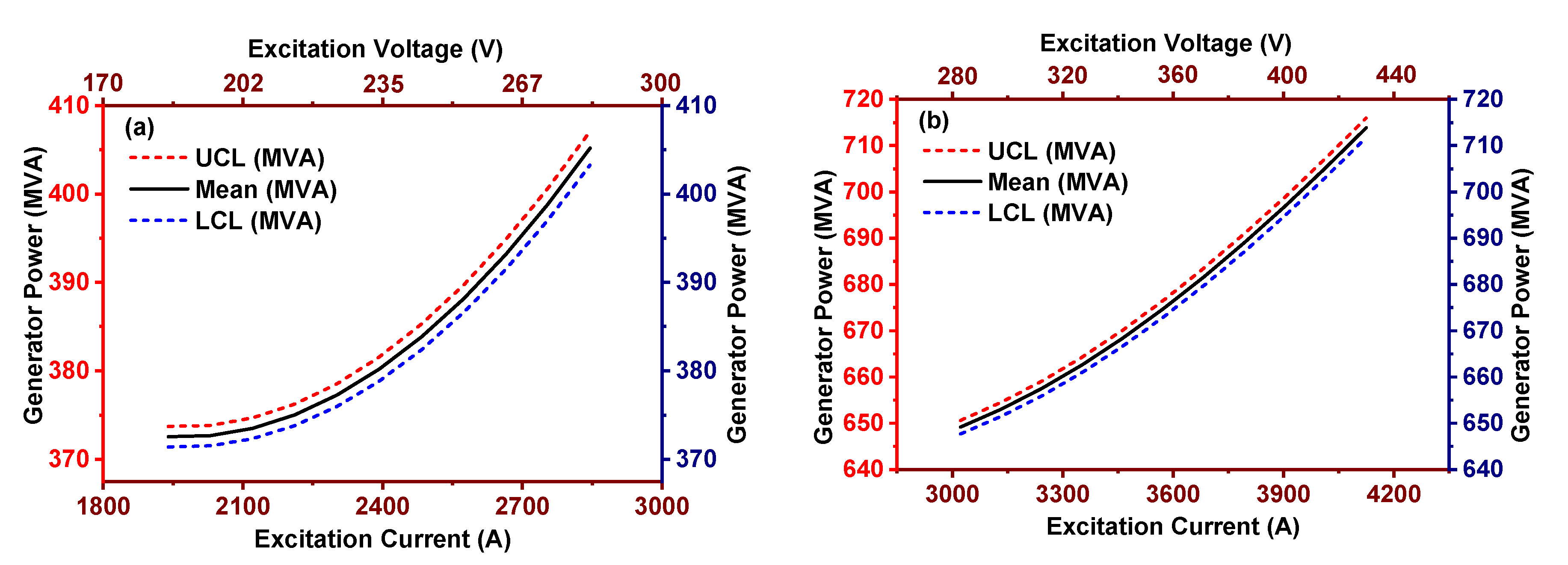
In order to evaluate the combined effect of excitation voltage and excitation current on the power generation from the generator at the sustained 50% and 100% unit load (resistive power in MW_e), the excitation voltage and excitation current are systematically increased from the minimum to maximum values, whereas the remaining thermo-electric operating parameters are maintained at the average values as mentioned in Table 6. Keeping the remaining thermo-electric operating parameters at the average values is essential to sustain the 50% and 100% unit load from the generator.

Figure 6a,b shows the combined effect of excitation voltage and excitation current on the generator power at 50% and 100% unit load.

A general increasing trend of generator power is observed with the increase in excitation voltage and excitation current. At 50% unit load, generator power is increased from 372.5 MVA to 405.2 MVA when excitation voltage and excitation current are changed from 186 V to 277V and 1940 A to 2845 A, respectively. At 100% unit load, generator power is increased from 649.2 MVA to 713.9 MVA when excitation voltage and excitation current change from 297 V to 431 V and 3022 A to 4124 A, respectively. With every 10V and 100A increase in excitation voltage and excitation current, the average relative increase in the generator power is 0.84% and 0.96% at 50%, and 100% unit load, respectively.

6.2. Generator Power Control during Coal Mill Trip Accident (Failure Mode Recovery and Mitigation of Cost of Failure)

The robust externally validated and flexible LSSVM process model is potentially applicable for predicting the system response under the power plant’s failure modes. Based on the model prediction, the strategies and standard operating procedures can be prepared to effectively deal with the abnormal and failure modes of the industrial operations without facing the actual accidents and failures, and thus, help minimize the operation cost. Moreover, the model response under the simulated operating parameters of the industrial operations provides the characteristics system response that, in turn, can be effectively useful for enhancing the operation control training of the workforce.

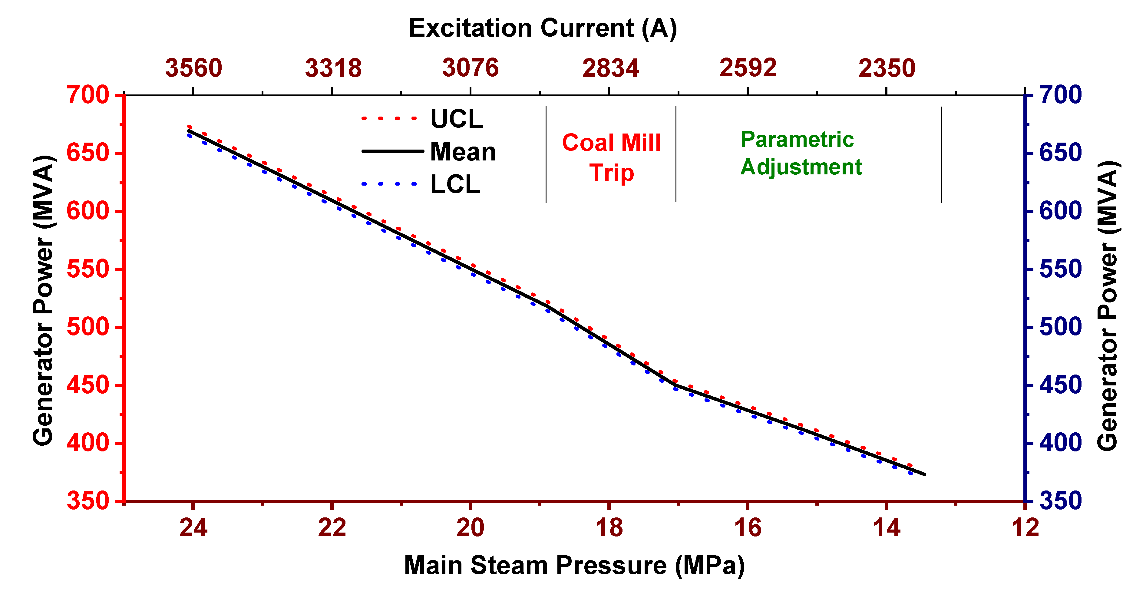
The coal mill trip is a potentially costly failure in the power plant operation that poses severe implications to the power complex’s safe and continuous power generation. Coal mill trip causes a sharp decrease in the total coal flowrate, and under the improper operation control of the boiler, the performance of heating surfaces (super-heater, re-heater, economizer) installed inside the boiler gets poor. Furthermore, under the sudden and considerable reduction in the fuel supply and improper operation control, the combustion and flame may get unstable or die out, leading to complete power loss from the unit. In this scenario, operators’ immediate action is to effectively control the power plant’s thermo-electric operating parameters to avoid the sharp drop in power production and restore power generation’s safe operation from the power complex.

Figure 7 shows the generator power trend against the main steam pressure and excitation current (two of the thermo-electric operating parameters). Generator power is commonly made to decrease from about 100% to nearly 50% generation capacity by the variation in the thermo-electric operating parameters based on the grid’s energy demand variation. A smooth declining gradient of the generator power generation trend from 669.5 MVA to 518.4 MVA is observed by the systematic variation in thermo-electric operating parameters. At the main steam pressure of 18.9 MPa, it is considered that a coal mill is tripped (accident), causing the abnormal variation in the thermo-electric operating parameters. As a result, generator power is decreased from 518.4 MVA to 450.4 MVA. The dip in the trend represents the coal mill operation failure and can be directly related to power, operation safety, and monetary costs. A set of adjustments in the thermo-electric operating parameters are made in computer-simulated Monte-Carlo experiments based on the discussions with operation engineers and literature review [32,56,57,58,59]. Insufficient adjustments and inefficient handling of thermo-electric operating parameters related to boiler and turbine operation may lead to complete power loss from the power plant. Five sets of computer-simulated experiments with potential solutions were prepared and tested on a robust and well-validated LSSVM process model of the power plant. One set of simulated experiments is successfully employed to ensure combustion stability and achieve a smooth and gradual 50% power generation capacity after the accident. The sharp decrease in generator power is highly avoidable as it affects the safe and smooth operation of the generator and the stability of the grid.

The generator power trend plotted by the LSSVM model in Figure 7 may also serve as the generator power’s performance curve during the coal mill trip scenario. The operation data based constructed process models can be potentially employed for preparing the operation strategies and scheme of action for the possible accidents that happen during the operation in industries. Therefore, the presented approach constitutes the one step ahead in advancing the industry 4.0 data analytics concept in the industrial operation for improved process control and efficient operation management practices.

6.3. Effect of Adjustment in Thermo-Electric Operating Parameters for Optimal Generator Power (A Case of AI for Operation Control Excellence Tool)

This section presents a detailed example of the validated LSSVM process model’s commissioning as an operational excellence tool based on its prediction for carefully designed computer simulated experiments.

Three actual operating conditions of the power plant at approximate 50% generation capacity are randomly selected. It is important to note that the power plant is operating under controlled operational conditions during this time. The set of values of operational parameters at these three randomly selected controlled operational states are shown in

Table 7. Summary of actual and adjusted thermo-electric operating parameters at 50% generation capacity.

Thermo-Electric Operating Parameters	Unit	50% Generation Capacity (MVA)
		Actual	Adjusted	Actual	Adjusted	Actual	Adjusted
Coal flow rate (Mc)	t/h	134	134	135	138	137	137
Air flow rate (Ma)	t/h	1519	1500	1508	1497	1531	1519
Water/Coal ratio (w/c)	-	7.46	7.43	8.05	7.8	7.69	7.43
Middle temp. (Tmid)	°C	354	357	366	368	353	356
LT Eco water outlet temp. (TLT.ECO)	°C	98	99	98	99	96	97
APH air outlet temp. (Ta)APH	°C	315	318	334	336	323	325
% O2 in flue gas at APH outlet (% O2)	%	7.98	7.90	7.60	7.55	7.63	7.59
Flue gas temp. after APH (Tfg)APH	°C	127	121	133	127	129	121
Ambient temp. (Tamb)	°C	15.0	15.0	12.0	12.0	27.0	27.0
Feed water pressure (FWP)	MPa	15.9	15.9	17.3	17.3	16.4	16.4
Feed water temp. (FWT)	°C	263	265	267	269	263	265
Feed water flow (FWF)	t/h	1004	996	1088	1076	1056	1043
Main steam pressure (MSP)	MPa	13.5	13.5	14.8	14.8	13.6	13.6
Main steam temp. (MST)	°C	550	566	551	566	551	566
Reheat pressure (RHP)	MPa	2.7	2.7	3.3	3.3	2.7	2.7
Reheat temp. (RHT)	°C	559	567	560	567	561	567
Absolute condenser vacuum (Pvac)	kPa	93.84	93.92	94.35	94.4	93.55	93.62
Deaerator temp. (Td)	°C	165	167	168	169	167	169
Attemperation water flow rate (AWF)	t/h	56	35	27	19	14	9
Condensate temp. (TC)	°C	34	34	32	32	36	36
Auxiliary power (Paux)	MWe	20.5	20.3	22.4	22.2	20.8	20.5
Turbine speed (N)	Rpm	3002	3002	3009	3009	3006	3006
Excitation voltage (Exc. V)	V	223	223	210	210	272	272
Excitation current (Exc. I)	A	2323	2323	2188	2188	2776	2776

. Similar tests are conducted to take the operational control data of thermo-electric operating parameters at 75% and the power plant’s 100% generation capacity.

Extensive literature review [32,56,57,58,59] and detailed critical discussions are conducted with operating engineers’ inter-discipline teams. Multiple options of computer-simulated experiments are designed to check the possible increase in generator power with the adjustments in thermo-electric operating parameters. The viable and possible adjustments designed in the thermo-electric operating parameters, considering the power plant’s operating conditions, are listed in Table 7,

Table 8. Summary of actual and adjusted thermo-electric operating parameters at 75% generation capacity.

Thermo-Electric Operating Parameters	Unit	75% Generation Capacity (MVA)
		Actual	Adjusted	Actual	Adjusted	Actual	Adjusted
Coal flow rate (Mc)	t/h	184	184	201	201	193	193
Air flow rate (Ma)	t/h	1983	1965	2142	2129	2064	2034
Water/Coal ratio (w/c)	-	7.73	7.61	8.04	7.95	7.7	7.58
Middle temp. (Tmid)	°C	383	385	401	405	378	382
LT Eco water outlet temp. (TLT.ECO)	°C	97	98	92	93	95	96
APH air outlet temp. (Ta)APH	°C	322	325	333	338	325	328
% O2 in flue gas at APH outlet (% O2)	%	6.76	6.70	6.25	6.21	6.67	6.53
Flue gas temp. after APH (Tfg)APH	°C	127	122	131	126	137	131
Ambient temp. (Tamb)	°C	8.0	8.0	10.0	10.0	27.0	27.0
Feed water pressure (FWP)	MPa	21.7	21.7	24.8	24.8	22.2	22.2
Feed water temp. (FWT)	°C	278	280	287	289	279	281
Feed water flow (FWF)	t/h	1424	1400	1613	1598	1487	1463
Main steam pressure (MSP)	MPa	17.7	17.7	20.4	20.4	18.2	18.2
Main steam temp. (MST)	°C	554	567	554	566	554	568
Reheat pressure (RHP)	MPa	3.4	3.4	4.06	4.06	3.7	3.7
Reheat temp. (RHT)	°C	560	567	560	567	563	567
Absolute condenser vacuum (Pvac)	kPa	95.24	95.32	94.51	94.6	92.74	92.82
Deaerator temp. (Td)	°C	174	175	180	181	174	176
Attemperation water flow rate (AWF)	t/h	33	12	39	25	19	12
Condensate temp. (TC)	°C	30	30	32	32	38	38
Auxiliary power (Paux)	MWe	25.1	24.9	25.7	25.4	25	24.7
Turbine speed (N)	Rpm	3001	3001	3001	3001	3003	3003
Excitation voltage (Exc. V)	V	269	269	285	285	296	296
Excitation current (Exc. I)	A	2757	2757	2904	2904	3012	3012

and

Table 9. Summary of actual and adjusted thermo-electric operating parameters at 100% generation capacity.

Thermo-Electric Operating Parameters	Unit	100% Generation Capacity (MVA)
		Actual	Adjusted	Actual	Adjusted	Actual	Adjusted
Coal flow rate (Mc)	t/h	243	243	239	239	248	248
Air flow rate (Ma)	t/h	2453	2418	2399	2399	2507	2470
Water/Coal ratio (w/c)	-	7.98	7.96	8.15	8.12	7.85	7.79
Middle temperature (Tmid)	°C	415	417	413	415	417	419
LT Eco water outlet temperature (TLT.ECO)	°C	92	93	91	92	95	96
APH air outlet temperature (Ta)APH	°C	340	346	336	343	338	346
% O2 in flue gas at APH outlet (% O2)	%	5.79	5.63	5.64	5.64	5.43	5.21
Flue gas temperature after APH (Tfg)APH	°C	133	130	134	129	148	135
Ambient temperature (Tamb)	°C	5.0	5.0	10.0	10.0	34.0	34.0
Feed water pressure (FWP)	MPa	29.7	29.7	29.6	29.6	29.5	29.5
Feed water temperature (FWT)	°C	297	299	297	299	297	300
Feed water flow (FWF)	t/h	1950	1935	1951	1936	1947	1935
Main steam pressure (MSP)	MPa	24.1	24.1	24	24	23.8	23.8
Main steam temperature (MST)	°C	553	567	552	566	553	568
Reheat pressure (RHP)	MPa	4.8	4.8	4.8	4.8	4.2	4.2
Reheat temperature (RHT)	°C	564	566	565	569	563	568
Absolute condenser vacuum (Pvac)	kPa	94.87	94.93	94.38	94.44	90.11	90.26
Deaerator temperature (Td)	°C	186	189	187	188	189	191
Attemperation water flow rate (AWF)	t/h	50	20	47	18	58	19
Condensate temperature (TC)	°C	31	31	33	33	46	46
Auxiliary power (Paux)	MWe	27.4	27.1	28.0	27.9	27.8	27.5
Turbine speed (N)	Rpm	2996	2996	3012	3012	3004	3004
Excitation voltage (Exc. V)	V	364	364	310	310	396	396
Excitation current (Exc. I)	A	3598	3598	3131	3131	3865	3865

. It is essential to mention here that the coal flow rate is essentially kept the same in the three power generation capacities to keep the same thermal energy spent. Moreover, the main steam pressure, reheat steam pressure, turbine speed, and excitation voltage are kept nearly unchanged at the sustained 50%, 75%, and 100% generation capacity of the power plant.

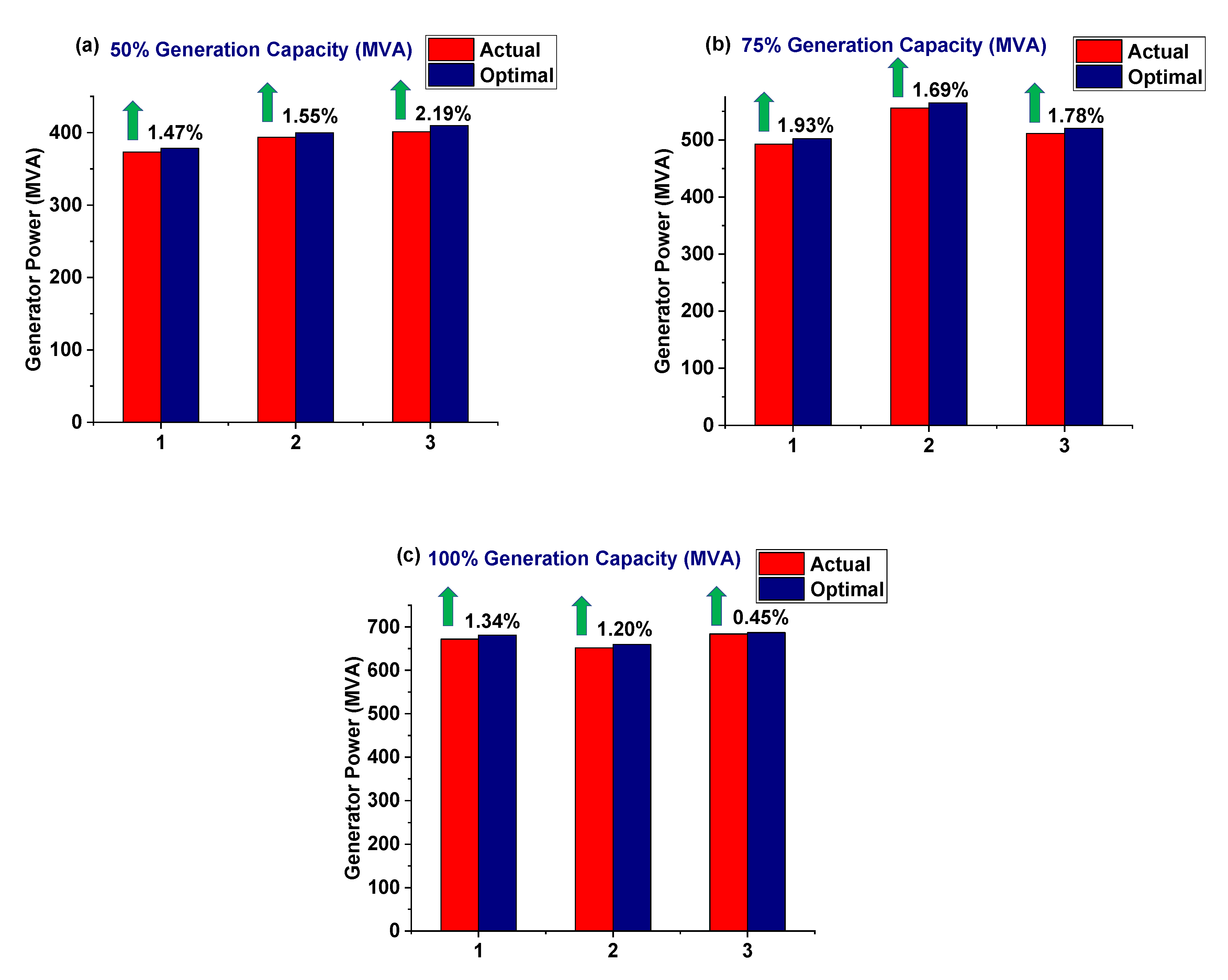
At 50% generation capacity, the generator power for the power plant’s three operating conditions under the adjusted thermo-electric operating parameters is increased by 1.47%, 1.55%, and 2.19%. For 75% and 100% generation capacity, the increase in generator power under the adjusted thermo-electric operating parameters are 1.93%, 1.69%, 1.78% and 1.34%, 1.20%, 0.45%, respectively. The average increase in generator power under the adjusted thermo-electric operating parameters is 1.74%, 1.80%, and 1.0% at 50% generation capacity, 75% generation capacity, and the power plant’s 100% generation capacity. These increases are illustrated in Figure 8.

As observed in Table 7, Table 8 and Table 9, many thermo-electric operating parameters during the power plant’s actual operation state lie in the lower controllable operating regimes. For example, the main steam temperature, reheat steam temperature, flue gas temperature after APH are generally near the lower controllable limits caused by the in-effective combustion control and reduced heat transfer to the heating surfaces. The adjustments made in the thermo-electric operating parameters lie within the manufacturer designed parametric operating limits for the power plant operation control that resulted in the optimal power production from the power plant. The data-driven optimization strategies for the improved operation control and operation excellency of the power plant are achieved by combining the experience of operation engineers of industries and the detailed analysis of AI-based process modeling conducted in the spirit of industry 4.0.

7. Conclusions

Based on the real operation data, the process modeling techniques, i.e., MLR, ANN, and LSSVM, are employed to model the generator power of 660 MW_e supercritical coal power plant.

The LSSVM has outperformed the MLR and ANN process models based on the validation test conducted on the unseen operation data taken from the power plant. The LSSVM has demonstrated reliable performance in modeling the generator power and thereby constructing the trend lines of the generator operation against the thermo-electric operating parameters of the power plant.

With every 10 V and 100 A increase in excitation voltage and current at 50% and 100% unit load, the average increase in generator power is 0.84% and 0.96%.

During the load decrement scenario from about 100% to nearly 50% generation capacity, the decrease in generator power after the coal mill trip accident is recovered as predicted by the LSSVM process model by a significant adjustment in the thermo-electric operating parameters.

At 50% generation capacity, the generator power for the three operating conditions of the power plant under the adjusted thermo-electric operating parameters is increased by 1.47%, 1.55%, and 2.19%, whereas for 75% and 100% generation capacity, the increase in generator power under the adjusted thermo-electric operating parameters are 1.93%, 1.69%, 1.78% and 1.34%, 1.20%, 0.45%, respectively.

The data-driven optimization strategies for the power plant’s improved operation control are achieved by the extensive and detailed discussions with the operating engineers and the analysis of AI-based process modeling conducted in the spirit of industry 4.0.

References

- Wang, Z. Random Forest based hourly building energy prediction. Energy Build. 2018, 171, 11–25. [Google Scholar] [CrossRef]
- Uddin, G.M.; Arafat, S.M.; Ashraf, W.M.; Asim, M.; Bhutta, M.M.A.; Jatoi, H.U.K.; Niazi, S.G.; Jamil, A.; Farooq, M.; Ghufran, M.; et al. Artificial Intelligence-Based Emission Reduction Strategy for Limestone Forced Oxidation Flue Gas Desulfurization System. J. Energy Resour. Technol. 2020, 142, 092103. [Google Scholar] [CrossRef]
- Márquez-Nolasco, A. Optimization and estimation of the thermal energy of an absorber with graphite disks by using direct and inverse neural network. J. Energy Resour. Technol. 2018, 140, 020906. [Google Scholar] [CrossRef]
- Askari, O. Fundamental study of spray and partially premixed combustion of methane/air mixture. J. Energy Resour. Technol. 2013, 135, 021001. [Google Scholar] [CrossRef]
- Yu, G.; Hadi, F.; Metghalchi, H. Rate-controlled constrained-equilibrium application in shock tube ignition delay time simulation. J. Energy Resour. Technol. 2019, 141, 020801. [Google Scholar] [CrossRef]
- Krzywanski, J. A Comprehensive Three-Dimensional Analysis of a Large-Scale Multi-Fuel CFB Boiler Burning Coal and Syngas. Part 1. The CFD Model of a Large-Scale Multi-Fuel CFB Combustion. Entropy 2020, 22, 964. [Google Scholar] [CrossRef]
- Glushkov, D.; Kuznetsov, G.; Paushkina, K. Switching coal-fired thermal power plant to composite fuel for recovering industrial and municipal waste: Combustion characteristics, emissions, and economic effect. Energies 2020, 13, 259. [Google Scholar] [CrossRef]
- Razzaq, L. Modeling Viscosity and Density of Ethanol-Diesel-Biodiesel Ternary Blends for Sustainable Environment. Sustainability 2020, 12, 5186. [Google Scholar] [CrossRef]
- Usman, M. Use of gasoline, LPG and LPG-HHO blend in SI engine: A comparative performance for emission control and sustainable environment. Processes 2020, 8, 74. [Google Scholar] [CrossRef]
- Najjar, M.K. Framework for a Systematic Parametric Analysis to Maximize Energy Output of PV Modules Using an Experimental Design. Sustainability 2019, 11, 2992. [Google Scholar] [CrossRef]
- Abokersh, M.H. A framework for the optimal integration of solar assisted district heating in different urban sized communities: A robust machine learning approach incorporating global sensitivity analysis. Appl. Energy 2020, 267, 114903. [Google Scholar] [CrossRef]
- Ximenes Naves, A. Economic Optimization of the Energy Supply for a Logistics Center Considering Variable-Rate Energy Tariffs and Integration of Photovoltaics. Appl. Sci. 2019, 9, 4711. [Google Scholar] [CrossRef]
- Escorihuela, L. Toward computational and experimental characterisation for risk assessment of metal oxide nanoparticles. Environ. Sci. Nano 2018, 5, 2241–2251. [Google Scholar] [CrossRef]
- Petoumenou, M.I. Comparison between bioconcentration factor (BCF) data provided by industry to the European Chemicals Agency (ECHA) and data derived from QSAR models. Environ. Res. 2015, 142, 529–534. [Google Scholar] [CrossRef] [PubMed]
- Gómez, S. Structural patterns in complex systems using multidendrograms. Entropy 2013, 15, 5464–5474. [Google Scholar] [CrossRef]
- Krzywanski, J. A comprehensive, three-dimensional analysis of a large-scale, multi-fuel, CFB boiler burning coal and syngas. Part 2. Numerical simulations of coal and syngas co-combustion. Entropy 2020, 22, 856. [Google Scholar] [CrossRef]
- Krzywanski, J. Heat Transfer Performance in a Superheater of an Industrial CFBC Using Fuzzy Logic-Based Methods. Entropy 2019, 21, 919. [Google Scholar] [CrossRef]
- Krzywanski, J. Fluidized Bed Jet Milling Process Optimized for Mass and Particle Size with a Fuzzy Logic Approach. Materials 2020, 13, 3303. [Google Scholar] [CrossRef]
- Sosnowski, M.; Krzywanski, J.; Scurek, R. A fuzzy logic approach for the reduction of mesh-induced error in CFD analysis: A case study of an impinging jet. Entropy 2019, 21, 1047. [Google Scholar] [CrossRef]
- Kabugo, J.C. Industry 4.0 based process data analytics platform: A waste-to-energy plant case study. Int. J. Electr. Power Energy Syst. 2020, 115, 105508. [Google Scholar] [CrossRef]
- Cheng, L.; Yu, T. A new generation of AI: A review and perspective on machine learning technologies applied to smart energy and electric power systems. Int. J. Energy Res. 2019, 43, 1928–1973. [Google Scholar] [CrossRef]
- Narciso, D.A.; Martins, F. Application of machine learning tools for energy efficiency in industry: A review. Energy Rep. 2020, 6, 1181–1199. [Google Scholar] [CrossRef]
- Kaytez, F. A hybrid approach based on autoregressive integrated moving average and least-square support vector machine for long-term forecasting of net electricity consumption. Energy 2020, 197, 117200. [Google Scholar] [CrossRef]
- Liu, Z. Empirical mode decomposition based hybrid ensemble model for electrical energy consumption forecasting of the cement grinding process. Measurement 2019, 138, 314–324. [Google Scholar] [CrossRef]
- Elfaki, E.A.; Ahmed, A.H. Prediction of electrical output power of combined cycle power plant using regression ANN model. J. Power Energy Eng. 2018, 6, 17. [Google Scholar] [CrossRef]
- Zhu, H. A power prediction method for photovoltaic power plant based on wavelet decomposition and artificial neural networks. Energies 2016, 9, 11. [Google Scholar] [CrossRef]
- Manobel, B. Wind turbine power curve modeling based on Gaussian processes and artificial neural networks. Renew. Energy 2018, 125, 1015–1020. [Google Scholar] [CrossRef]
- Bilal, B. Wind turbine power output prediction model design based on artificial neural networks and climatic spatiotemporal data. In Proceedings of the 2018 IEEE International Conference on Industrial Technology (ICIT), Lyon, France, 19–22 February 2018. [Google Scholar]
- Zendehboudi, A.; Baseer, M.; Saidur, R. Application of support vector machine models for forecasting solar and wind energy resources: A review. J. Clean. Prod. 2018, 199, 272–285. [Google Scholar] [CrossRef]
- De, S. Development of an artificial neural network model for the steam process of a coal biomass cofired combined heat and power (CHP) plant in Sweden. Energy 2007, 32, 2099–2109. [Google Scholar] [CrossRef]
- Smrekar, J. Development of artificial neural network model for a coal-fired boiler using real plant data. Energy 2009, 34, 144–152. [Google Scholar] [CrossRef]
- Smrekar, J. Prediction of power output of a coal-fired power plant by artificial neural network. Neural Comput. Appl. 2010, 19, 725–740. [Google Scholar] [CrossRef]
- Gu, H. Optimized scheme in coal-fired boiler combustion based on information entropy and modified K-prototypes algorithm. Results Phys. 2018, 9, 1262–1274. [Google Scholar] [CrossRef]
- Wan, X. Research on Application of Big Data Mining Technology in Performance Optimization of Steam Turbines. In Proceedings of the CSEE, Wuhan, China, 12–15 March 2016. [Google Scholar]
- Cai, J.; Ma, X.; Li, Q. On-line monitoring the performance of coal-fired power unit: A method based on support vector machine. Appl. Therm. Eng. 2009, 29, 2308–2319. [Google Scholar] [CrossRef]
- Uddin, G.M. Monte Carlo study of the molecular beam epitaxy process for manufacturing magnesium oxide nano-scale films. IIE Trans. 2015, 47, 125–140. [Google Scholar] [CrossRef]
- Chi, Z.; Wu, J.; Yan, H. Handwritten numeral recognition using self-organizing maps and fuzzy rules. Pattern Recognit. 1995, 28, 59–66. [Google Scholar] [CrossRef]
- Kohonen, T. The Self-Organizing Map. Proc. EEE 1990, 78, 1464–1480. [Google Scholar] [CrossRef]
- Marks, K.M. Analysis of VLSI process data based on self-organizing feature maps. Proc. Nuero-Nimes 1988, 78, 337–347. [Google Scholar]
- Jomnonkwao, S.; Uttra, S.; Ratanavaraha, V. Forecasting road traffic deaths in Thailand: Applications of time-series, curve estimation, multiple linear regression, and path analysis models. Sustainability 2020, 12, 395. [Google Scholar] [CrossRef]
- Uyanık, G.K.; Güler, N. A study on multiple linear regression analysis. Procedia-Soc. Behav. Sci. 2013, 106, 234–240. [Google Scholar] [CrossRef]
- Lv, Y. Adaptive selective catalytic reduction model development using typical operating data in coal-fired power plants. Energy 2020, 192, 116589. [Google Scholar] [CrossRef]
- Tunckaya, Y.; Koklukaya, E. Comparative prediction analysis of 600 MWe coal-fired power plant production rate using statistical and neural-based models. J. Energy Inst. 2015, 88, 11–18. [Google Scholar] [CrossRef]
- Suykens, J.A. Weighted least squares support vector machines: Robustness and sparse approximation. Neurocomputing 2002, 48, 85–105. [Google Scholar] [CrossRef]
- Krzywanski, J. A general approach in optimization of heat exchangers by bio-inspired artificial intelligence methods. Energies 2019, 12, 4441. [Google Scholar] [CrossRef]
- Haykin, S. Neural Networks: A Comprehensive Foundation, 2nd ed.; Prentice-Hall Inc.: New Jersey, NJ, USA, 2007. [Google Scholar]
- Krzywanski, J. A generalized model of SO2 emissions from large-and small-scale CFB boilers by artificial neural network approach: Part 1. The mathematical model of SO2 emissions in air-firing, oxygen-enriched and oxycombustion CFB conditions. Fuel Process. Technol. 2015, 137, 66–74. [Google Scholar] [CrossRef]
- Dach, J. The use of neural modelling to estimate the methane production from slurry fermentation processes. Renew. Sustain. Energy Rev. 2016, 56, 603–610. [Google Scholar] [CrossRef]
- Uddin, G.M.; Arafat, S.M.; Kazim, A.H.; Farhan, M.; Niazi, S.G.; Hayat, N.; Zeid, I.; Kamarthi, S. Artificial intelligence-based Monte-Carlo numerical simulation of aerodynamics of tire grooves using computational fluid dynamics. AI EDAM 2019, 33, 302–316. [Google Scholar] [CrossRef]
- Klein, A. Fast Bayesian Optimization of Machine Learning Hyperparameters on Large Datasets. In Artificial Intelligence and Statistics; PMLR: Fort Lauderdale, FL, USA, 2017. [Google Scholar]
- Chen, P.-H.; Fan, R.-E.; Lin, C.-J. A study on SMO-type decomposition methods for support vector machines. IEEE Trans. Neural Netw. 2006, 17, 893–908. [Google Scholar] [CrossRef]
- Fan, R.-E.; Chen, P.-H.; Lin, C.-J. Working set selection using second order information for training support vector machines. J. Mach. Learn. Res. 2005, 6, 1889–1918. [Google Scholar]
- Platt, J. Sequential Minimal Optimization: A fast Algorithm for Training Support Vector Machines; Microsoft: Wshington, DC, USA, 1998. [Google Scholar]
- Uddin, G.M. Monte Carlo study of the high temperature hydrogen cleaning process of 6H-silicon carbide for subsequent growth of nano scale metal oxide films. Int. J. Nanomanufacturing 2013, 9, 407–430. [Google Scholar] [CrossRef]
- Uddin, G.M. Neural networks assisted computational aero-acoustic analysis of an isolated tire. Proc. Inst. Mech. Eng. Part D J. Automob. Eng. 2020, 234. [Google Scholar] [CrossRef]
- Rosen, M.A.; Tang, R. Improving steam power plant efficiency through exergy analysis: Effects of altering excess combustion air and stack-gas temperature. Int. J. Energy 2008, 5, 31–51. [Google Scholar] [CrossRef]
- Si, N. Exergy analysis of a 1000 MW double reheat ultra-supercritical power plant. Energy Convers. Manag. 2017, 147, 155–165. [Google Scholar] [CrossRef]
- Regulagadda, P.; Dincer, I.; Naterer, G. Exergy analysis of a thermal power plant with measured boiler and turbine losses. Appl. Therm. Eng. 2010, 30, 970–976. [Google Scholar] [CrossRef]
- Narula, R.; Koza, D.; Wen, H. Impacts of steam conditions on plant materials and operation in ultra-supercritical coal power plants. In Ultra-Supercritical Coal Power Plants; Elsevier: Amsterdam, The Netherlands, 2013; pp. 23–56. [Google Scholar]
Publisher’s Note: MDPI stays neutral with regard to jurisdictional claims in published maps and institutional affiliations. |
© 2020 by the authors. Licensee MDPI, Basel, Switzerland. This article is an open access article distributed under the terms and conditions of the Creative Commons Attribution (CC BY) license (http://creativecommons.org/licenses/by/4.0/).