Abstract
Ethanol is a widely produced fuel, as well as a fuel additive. Its price is closely related to the price of gasoline, its major substitute. This paper focuses on the impacts of the related variables on regional ethanol prices. Additionally, the length of the price dataset made it possible to isolate the impacts of COVID-19 on the ethanol prices. Using multiple regression and Confirmatory Factor Analyses, we found no significant correlation between the European and US ethanol prices because the major influencing factors were regionally different. In the case of the European ethanol markets, the positive factors were wheat, maize, and potassium chloride prices, while the European sugar and diammonium phosphate prices were negative. In the US markets, gasoline, sugar, and most of the artificial fertilizer prices were positive, while wheat prices were negative. Based on factor analysis, artificial fertilizers and maize factors proved to be important to the European markets, while US ethanol prices were driven by the crude oil-gasoline and raw materials factors. The COVID variable showed no significant connection with the EU prices, but negatively affected the US ethanol prices. This is explained by the different market characteristics, as the US is not only the major consumer, but also the major producer of the different oil products. Therefore, COVID-19 had a double effect on their oil and ethanol markets.
1. Introduction
The fossil energy resources of the Earth are finite, and their continued use causes evermore damage to the environment through global warming and pollution [1]. Within a very short period of time, humanity must switch to the use of renewable energy sources, preferably by incorporating the concept of a circular economy, with as little further waste and degradation to soil, water, and air as possible [2,3,4]. Energy is a key issue in the world economy, especially in the transportation sector. As of this moment in time, biofuels show great promise as direct fuel substitutes. Currently, first-generation production methods are in use. Although second-generation production technologies are already available in an immature state, they are expensive compared to the first-generation technology. The International Energy Agency (IEA) has highlighted the importance of biofuels and ethanol in particular: “Modern bioenergy is the overlooked giant of renewables. Bioenergy is particularly important in decarbonizing transport and there is untapped potential for bioenergy in the transport sector. Biofuels are a leading pathway to decarbonize transport. Biofuels and electric mobility are complementary options in decarbonizing transport. There is significant untapped potential in ethanol” [5].
The ethanol industry, and thus the demand for ethanol, is mostly driven by the mandatory blending mandates. This links the use of ethanol directly to that of gasoline, so their prices should normally move together. The major issue with the ethanol industry is the product price and its influencing factors. The former determines the price competitiveness of the ethanol, while the latter shows any factors which have a measurable impact on the ethanol prices. In this article, we included crude oil prices (West Texas Intermediate WTI and BRENT), conventional (New York Harbor & Gulf Coast) and regular gasoline prices, related raw materials and commodity prices (corn, wheat, barley, and sugar), and prices of different artificial fertilizers. Our initial hypothesis was straightforward. The major impact of COVID-19 was reduced mobility, which directly decreased gasoline use. Lower demand, ceteris paribus, results in lower prices. In an extreme case, this could be even negative as experienced in April [6]. Lower gasoline prices negatively influenced the raw material prices through the loss of a significant part of demand. Researchers, as well as research institutions, expected the same price movement, although to a different extent [7,8].
Our research aims were to provide an overview of the major ethanol markets (the US and the EU) and to identify their most important driving forces. More specifically, we determined the key variables of the regional price changes and measured their impacts on the ethanol prices. The major contribution of this article to the existing literature is the use of real price data, which made it possible to separate the impacts of the COVID-19 pandemic on the ethanol prices. This is a logical continuation of the corresponding articles in this field based on modelling results and different forecasts.
First, we introduce the most relevant tendencies of the global market of ethanol, of oil, and of the most important raw materials (maize, sugarcane). Then, we examine the correlations of their prices and the previous literature about the effects of COVID-19 on these markets. Following this, we analyze the connections between the EU and US ethanol prices, as well as the impacts of their major influencing factors. The effects of COVID-19 on the ethanol prices were estimated by factor analysis. The final chapter concludes our findings.
2. Literature Review
2.1. Global Ethanol Markets
The global biofuel market substitutes 2.32–5% of oil consumption using 71 million hectares of arable land [9,10]. Within the biofuels, ethanol production is more significant than biodiesel, with ethanol production reaching 110 billion liters in 2018. Its major producers are the US (2018: 54% share, the major raw material is corn) and Brazil (2018: 30% share, the major raw material is sugarcane) [11]. The share of further, nonfood-based, second-generation ethanol production is negligible (0.4%, 0.4 billion l/year), although this is expected to increase remarkably in the future, e.g., it may double by 2023 [12,13,14,15]. This results in different raw materials, most notably agricultural co-products. These are cobs and stover in the US and China, sugarcane bagasse and straw in Brazil, and molasses in India. Approximately 80% of globally produced ethanol is used as fuel, followed by food, pharmaceutical, and cosmetics industrial purposes [16,17].
Global ethanol production has increased almost continuously with the exception of 2012, due to the high sugar prices. This growth slowed in the last 5 years to 2% per year on average [11].
The major cost item of the corn-based ethanol production is the raw material, which reached up to 59%, based on the 13-year Iowa State time period [18]. Excluding depreciation, this share went up to 85–95%, which proves that depreciation is the second largest cost item in the ethanol industry, due to the high initial investment need. Changes in the price ratio of maize and ethanol are subject to significant uncertainty, and this fundamentally determines the profitability of ethanol production (Figure 1).
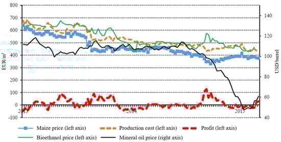
Figure 1.
Connections between the major factors of the ethanol price. Source: [19].
Ethanol production provides not only additional demand for the maize production, e.g., 40% of the total maize production in the US is used for ethanol production, but also results in high value-added products. The price of ethanol in the US is 55% higher than the price of maize, due to the use of the dry milling process. The major items of this surplus are the coproducts that can be used in the livestock industry as a valuable and relatively cheap forage. Employment is another economic contribution that comes from the ethanol industry. In the US, every 1 million liters of ethanol produced results in six workplaces, increases the GDP and governmental taxes by USD 754,000 and USD 164,000, respectively [11].
The major coproduct is the distiller’s dried grain with solubles (DDGS) that is priced favorably when compared to either maize or soybean meal prices (Figure 2).
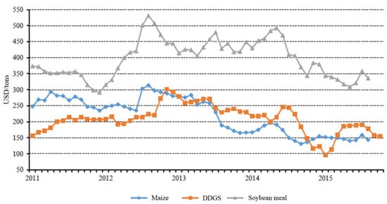
Figure 2.
Evolution of maize, distiller’s dried grain with solubles (DDGS), and soybean meal prices. Source: [19].
According to market forecasts, the ethanol market is estimated to reach USD 33.7 billion in 2020. This is expected to double by 2025, with a 14% Compound Annual Growth Rate (CAGR), resulting mainly from the spread and increase of mandatory blending objectives [20]. This is supported by the low production costs (USD 0.180–0.79/L) that make production typically competitive with both the oil (September 2020: BRENT: USD 0.3/L) and biodiesel costs (USD 0.670–0.9/L) when sugarcane and maize are used as raw materials [5,21,22,23]. However, the approximately 30% lower energy density of ethanol should be taken into account.
The exportation of maize and sugarcane negatively impact ethanol production [24]. Due mainly to the environmental regulations and the limited quantity of raw materials, the share of further ethanol generations (e.g., cellulose-based) is expected to grow [25,26].
Ethanol prices differ remarkably in the EU and in the US, as different raw materials and technologies are used. Regarding the EU, the average price in the last 5 years was USD 0.54/L and showed a slight increase during the analyzed period. Meanwhile, in the US, the average price was only USD 0.32/L and showed a decreasing trend (Figure 3). The average price difference is 40% (between 22% and 66%), which influences their competitiveness on the regional ethanol markets. Another important trend is the widening price gap between these two regional markets.
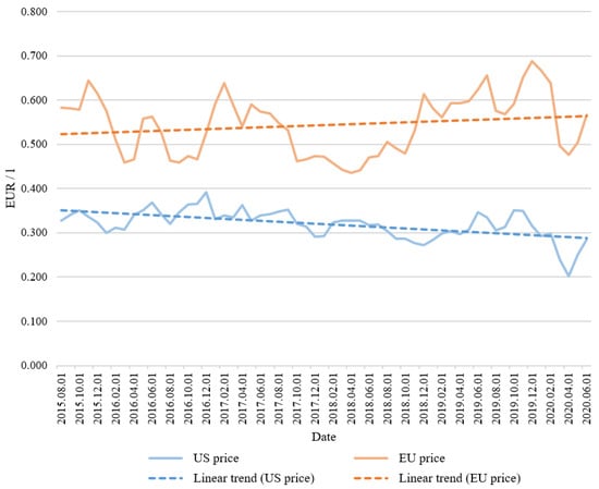
Figure 3.
Ethanol prices in the US and EU. Source: [27].
2.2. The Impacts of Oil Market on the Ethanol, Maize and Food Prices
Energy is a strategic product, which, in this decade, has had a yearly 1.5% average consumption growth rate [28]. Oil fulfills a major part of the current global energy requirements. Its production increased in the last two decades, and reached 5.5 trillion liters in 2019, while consumption has also increased over the years and was 5.8 trillion liters within the same year [29]. Due to the COVID-19 pandemic, which reduced mobility, consumption is expected to decrease to 5.3 trillion liters in 2020 [30]. This has a significant impact on the prices, as well as on the development of the world economy. Long-term forecasts anticipate further growth of the global demand (8.1 trillion liters in 2040), especially in developing countries [31]. According to Van der Ploeg (2011) [32], oil-rich countries generally have a low GDP/capita value, due to the lack of diversification, price fluctuations, political rent-seeking, and geopolitical risks. Majumder et al. (2020) [33] argued that trade liberalization would greatly reduce the impacts of this resource.
Changes in oil prices showed a high correlation with food prices up until 2017, while they moved in the opposite direction in 2017 and 2018 (Figure 4). Alghalith (2010) [34] found that the increase of the oil price by UD 1 resulted in a 5.6-point-higher food price index on average.
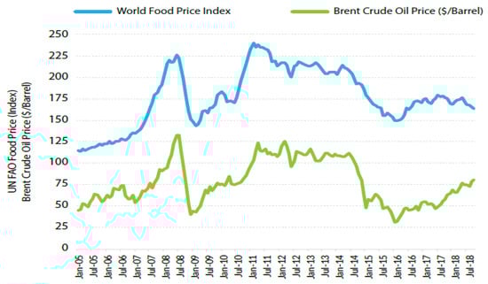
Figure 4.
Connection between the world food price index and the BRENT crude oil price. Source: [11].
Nazlioglu (2011) [35] found that oil prices have a nonlinear relationship with not only the price of food, but also with maize and soybean prices, using nonlinear causality analysis. He also argued that oil prices can forecast the price of food. However, it should be noted that only 15% of the food price is the cost of raw material in the US [11], but food price changes are the major food security risk in developing countries [36].
Trujillo-Barrera et al. (2012) [37] found a weaker connection between oil and maize prices than between maize and ethanol prices in the US. Natanelov et al. (2013) [38] pointed out that the latter was also strengthened by the US governmental fuel policy in the analyzed 2006–2011 period. The variability of the maize prices was greater than that of the ethanol or crude oil prices (Figure 5). This was caused by the significant maize demand of the ethanol industry and the relatively high oil prices, which made ethanol production competitive.
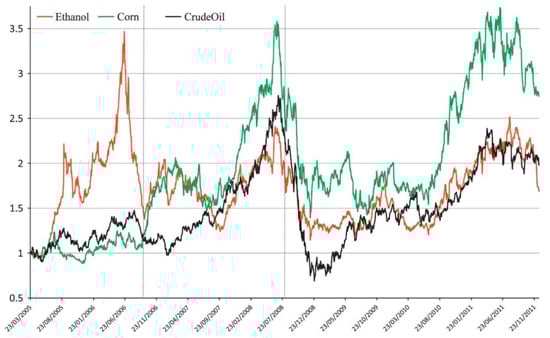
Figure 5.
Evolution of the ethanol, corn, and crude oil prices. Source: [38].
Dong (2019) [39] analyzed the long-term connection between oil and maize prices (Figure 6). According to his results, (1) oil prices had a one-way impact on maize prices, (2) the technological developments strengthened this connection and decreased the growth of maize prices, (3) there is a certain oil price limit where this connection disappears, and (4) this is the reason why changes in oil prices impact food prices.
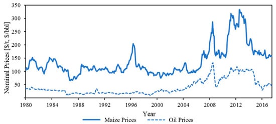
Figure 6.
Connection between maize and oil prices, 1980–2017. Source: [39].
Bahel et al. (2013) [40] stated that the major limitation of ethanol production in the 1990s was the low price of oil, but this accelerated in 1999–2008 due to the significant increase of the price of oil. They also pointed out that the main reason for the positive correlation between the biofuels and food prices is the rivalry for the limited area of arable land. The inelastic demand for food and the efficient use of arable land decrease the price of food in the short run, but the depletion of fossil energy resources increases food prices in the long run.
2.3. The Major Raw Materials of Ethanol Production
Almost 60% of ethanol is produced from maize, 25% from sugarcane, 7% from molasses, 4% from wheat, and the rest from other cereals, manioc, or sugar beet [41]. The raw material used is determined by the climate conditions of the given country or region. Manochio et al. (2017) [42] found that sugarcane-based ethanol production is 50–60% cheaper than that of maize-based production. They also highlighted that economically, sugarcane seems to be the best option, but significant governmental support can also make maize or sugar beet competitive, especially in the EU and the US [42]. This is the reason why the US has become the world’s major ethanol producer.
Another important aspect is the use of fertilizer. Its price shows a rising trend, mostly due to the fluctuations in the price of natural gas and the increase of production of maize ethanol [43]. Higher maize yields are directly linked to the higher use of fertilizer. According to Ott (2012) [44], there is a strong correlation between the prices of fertilizer and food, but food prices affect fertilizer prices, not vice versa. Higher food prices cause a higher demand for fertilizers. Energy is a key input in the production of fertilizers (mainly in case of nitrogen fertilizers), so the volatility of oil prices has a great influence on fertilizer costs and prices [44].
Mojović et al. (2009) [45] found that the conversion rate of sugarcane is only one-fifth or one-sixth than that of maize or wheat, but due to its exceptionally high yield and low production cost, this raw material results in a cheaper ethanol production cost and lower area needs, as well as greenhouse gas (GHG) emissions.
The major characteristics of the two most important raw materials, maize and sugarcane, are organized in two subchapters.
2.3.1. Maize
The expected maize production area in 2020 will be 196 million hectares globally with 5.9–6.0 tons/ha average yield, which will result in 1170 million tons of production [46]. The US has a key role in global production. Its global share of more than one-third demonstrates this, with a yield double that of the world average (Figure 7).
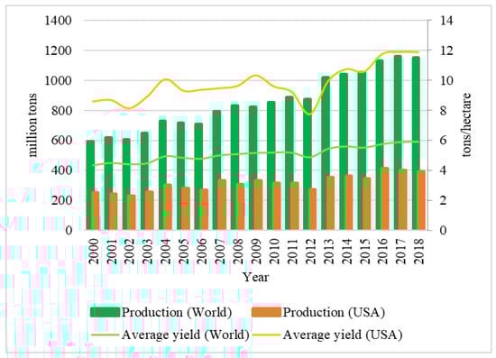
Figure 7.
World and US maize production and yield, 2000–2018. Source: [47].
The increasing US maize production is partly driven by increased ethanol production. According to the regulations, roughly 40% of the maize production is converted into ethanol and used in gasoline that has a 10% ethanol content (E10) [48].
2.3.2. Sugarcane
Brazil produced 40% of the global sugarcane in the last couple of years (Figure 8).
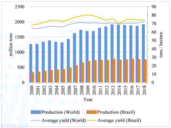
Figure 8.
World and Brazilian sugarcane production and yield, 2000–2018. Source: [47,49].
Larger production areas and higher yields have led to this increase in production. Soil compaction and soil degradation caused by heavy agricultural machinery negatively affected the Brazilian yield, which can be observed in 2008. Sugarcane-based ethanol production shows a high positive correlation with sugarcane exportation as a raw material (Table 1). In contrast, the exportation and production of cane sugar, the final product of sugarcane, correlates negatively with ethanol production [50].

Table 1.
Correlations (r) of sugarcane and cane sugar exports with ethanol production.
2.4. The Impacts of the COVID-19 Pandemic
It is a fact that the global oil demand decreased significantly this year due to the COVID-19 pandemic [51]. According to the IEA oil market report, reduced mobility affected gasoline consumption and diesel consumption, which is highly related to transport activities, while the aviation sector has almost collapsed due to the pandemic—in April, the total aviation distance was 80% less than that of the last year. Bassols and Bassols (2020) [52] stated that the petroleum demand dropped remarkably due to COVID-19, with demand even being negative during April. Due to this strong correlation, any measures (e.g., home office) against the further spread of the virus are going to lower oil prices even further. This scenario, ceteris paribus, makes biofuels production uncompetitive, especially in countries with higher production costs, which basically means every country with the exception of Brazil [24]. Although the demand of different oil products increased remarkably from May to August 2020, the second wave of the pandemic has caused significant, regionally different fluctuations in gasoline markets. This may be particularly true if the members of OPEC (Organization of the Petroleum Exporting Countries) do not significantly limit their production [30].
It should be noted that the demand of conventional fuel, in general, is expected to decrease more than the demand of biofuel, especially in Brazil and the EU [7]. This can be explained by the use of high-ethanol blends, which have not yet been introduced in the US.
The different impacts of the COVID-19 pandemic were already analyzed on a country/regional level, and commodity level. Kim et al. (2020) [53] underlined that the coronavirus pandemic increased food security risks in Asia and the Pacific. According to their study, there was a two-stage impact. Due to mobility restrictions, labor shortages, and income losses, domestic markets faced decreased production and consumption. Additionally, this decrease was made more severe by international export restrictions, which made it difficult to import certain food items. One of their interesting remarks was the comparison of the COVID-19 pandemic with the food crisis of 2007–2008. While the latter was more of a demand-side crisis (e.g., rapid global economic growth, increased biofuels production or the depreciation of the US dollar), the recent crisis is a supply-driven one because of the quarantine and lockdown measures.
Based on the price reactions, and thereby revenue changes, caused by COVID-19, Hart et al. (2020) [54] estimated the economic impact of this pandemic on Iowa’s corn, soybean, ethanol, pork, and beef markets. Iowa is the second-largest US agricultural state. In the case of ethanol, production losses (lower or even no production) were also taken into account. According to their results, the loss of the corn sector was about 788 million USD, while 213 million for the soybean, and 2.9 billion USD for the ethanol sector. The link between corn/soybean and the animal sectors is distillers’ grains (from corn-based ethanol processing) and soybean meal (from soybean-based biodiesel processing). As the production of biofuels decreased, the amount of these co-products also decreased, and livestock producers needed other types of fodder. The aggregated annual damage of the analyzed livestock sectors was roughly 2.8 billion USD. Country level impact analyses were also published, e.g., Shruthi and Ramani (2020) [55] on the Indian commodity markets or Barichello (2020) [56] on the Canadian agriculture and food sector. It can also be seen that the COVID-19 pandemic is an even larger problem for most of the middle-income countries where agriculture is a more significant contributor to the GDP [57].
The impacts are different depending on the sizes of the businesses also. According to Shretta (2020) [58], small and medium-sized firms suffered more from this pandemic, especially those that use intermediate goods from the affected parts of the world with limited alternative sources.
According to the World Trade Organization, the COVID-19 pandemic is likely to cause a 1332% fall in world trade [59]. The most heavily affected sector is services. Recovery is expected, but its speed depends on the length of the outbreak and the impacts of the emergency policy measures applied. However, forecasts and modelling results seem to be ambiguous at the commodity level. Using the Aglink-Cosimo model, a recursive-dynamic partial equilibrium model, Elleby et al. (2020) [7] found that the prices of agricultural commodities decreased sharply during the pandemic. Regarding the derived products, this decrease is predicted to grow even larger, especially for the biofuels. They anticipated a 15.9% decrease for biodiesel and a 13.8% decrease for ethanol in 2020. It is worth mentioning that the price of maize will decrease by only 7.2%, followed by a 9.7% drop in 2021. Price changes will lead to a production decrease. However, the change of production is expected to be smaller than that of the prices, due to the inelastic demand for agricultural commodities and the fixed nature of the production in the short run [7]. At the regional level, the EU and the US will face a higher biofuels’ price decrease than the other significant producers, Brazil and China. The World Bank’s forecast [8] shows that agricultural commodities are “pandemic-resistant” due to their lower sensitivity to economic activity. The difference between these two estimations on commodity price changes, i.e., those by the authors of [7,8], could be due to the different measurement of the use of the biofuels. Based on the latest agricultural outlook of the Organisation for Economic Co-operation and Development/Food and Agricultural Organization (OECD/FAO) [41], the major crops for ethanol production are corn (64%) and sugarcane (26%). According to that study, global ethanol production accounts for roughly 19% of the actual sugarcane production and 16% of the corn production. By 2029, the sugarcane production is anticipated to grow to 25%, while corn production is expected to decrease to 14%. However, different policy measures (e.g., export bans) implemented may affect food security. Sperling et al. (2020) [60] carried out expert interviews and obtained that the recovery process (post-COVID-19) should be based on the spread of advanced production technologies (e.g., digitalization, precision farming, or biotechnologies) to achieve a resilient and sustainable food system.
Although the COVID-19 pandemic has caused many problems, these problems have resulted in the creation of new, innovative solutions. One of the innovative solutions is the use of algae oil (as a type of biofuel) in nasal sprays, which can possibly prevent the spread of the virus [61]. Another promising idea is the use of jatropha extract against the coronavirus due to its strong antiviral characteristics [62].
3. Materials and Methods
The research aimed to analyze the major influencing factors on ethanol prices with particular attention paid to the impact of COVID-19. The most effective way to do this was to use multiple regression, if the model conditions were met. In regard to the quantity of variables, it could be useful to examine whether they can be grouped into background variables, which may provide the opportunity for a more detailed analysis. Similarly to Black-Babin (2019) [63], Ge-Wu (2019) [64], and Ciulla-D’Amico (2019) [65], we used multiple regression and Exploratory Factor Analyses (EFA) models. We ran these models with and without the COVID variable to measure the impacts of the pandemic. This was a dummy variable, and every month before 2020 was coded with 0, while the last 6 months were coded with 1. This provided many advantages by enabling us to measure not only the direct impact of COVID-19 on ethanol prices, but also the changes in the impact of the other variables compared to the hypothetical, no-COVID scenario. Miao (2013) [66] modelled the land use change effects of ethanol plants in the same way.
We used monthly average ethanol prices from Rotterdam and Chicago between August 2015 and June 2020. Our research explored all the major factors influencing the European and the US ethanol prices based on the dataset of Platts Europe (2020) [27].
The applied multivariate regression model was the following [67]:
where y is the dependent variable; β1, β2…βm are the independent variables; β0 is the constant; and ε is the error term.
y = β0 + β1x1 + β2x2 + … + βmxm + ε
We verified the parameters with the t-test. Upon further testing of the model, we checked whether the residues were normally distributed and ensured they did not show heteroscedasticity and multicollinearity [68]. Since the variables were normally distributed, Exploratory Factor Analyses (EFA) was used to verify whether these variables can be grouped together or not. According to the EFA, these groups could be confirmed to be acceptable by different tests. Then, the connection between these groups and the ethanol prices was analyzed. Instead of principal component analysis (see e.g., [69]), we used factor analysis, because a certain causal model could be identified in the background [70,71].
The following steps were carried out during our analysis:
- Bivariate correlation analysis for identifying the connections between the variables;
- Multiple regression using all the variables, and a separated regression model with and without the COVID variable;
- Identification of the background variables with CFA;
- Multiple regression with the verified factors as independent variables with and without the COVID variable.
The identified factors were:
- Crude oil prices (WTI and BRENT) (Source: EIA, 2020 [72])
- Gasoline prices (Source: EIA, 2020 [72])
- Conventional gasoline prices, New York Harbor
- Conventional gasoline prices, Gulf Coast
- Regular gasoline prices
- Grains (Source: World Bank Commodity Price Data (Pink Sheet Data), 2020 [73]):
- Wheat prices
- Barley prices
- Maize prices
- Sugar prices (European, US, and world prices) (Source: World Bank Commodity Price Data (Pink Sheet Data), 2020 [73])
- Prices of different artificial fertilizers (Source: World Bank Commodity Price Data (Pink Sheet Data), 2020 [73])
Our variables showed a normal distribution at a 5% significance level, which was considered favorable for the analysis. We tested normality with the Kolmogorov–Smirnov test.
Using the COVID variable, we obtained a categorical variable in our model. This was in line with our initial hypothesis that the change in the price of ethanol could also be explained using qualitative variables [73]. Due to this dummy variable, our model changed to the following form:
where D is a bivariate (0 and 1) variable, while X is a non-bivariate variable. Moreover, a Z variable was also created, and Z = DX.
Y = α + β1D1 + β2X + β3Z + e,
Implementing interactions between the bivariate and non-bivariate variables, we obtained different curve slopes. We had two different regressions for D = 0 and D = 1 cases, suggesting that they had different axis touching points and curve slopes. This implies that the marginal effect of X on Y is different when D = 0 and D = 1 [74]. Nonparametric correlation analysis also indicated the different nature of the variables (bivariate and non-bivariate). In the case of scale variables, Pearson correlation was applied.
In the factor analysis model, we assumed that our variables could be described by a linear combination of the factors (hypothetical background variables). Initially, the Kaiser-Meyer-Olkin (KMO) measure of sampling adequacy and Bartlett’s test of sphericity with oblimin rotation were used to test the null hypothesis that the variables are uncorrelated in the population. We used SPSS 25 software for the calculations.
4. Results and Discussion
4.1. Interrelations between the Variables
Both Rotterdam and Chicago prices showed normal distribution (p ethanol EUR = 0.250; p ethanol US = 0.877) based on the Kolmogorov–Smirnov test. Table 2 summarizes the descriptive statistics of the two price data sets (Rotterdam—EU, and Chicago—US).
Table 2.
Descriptive statistics of the price datasets.
According to our results, there was no significant correlation between the European and the US ethanol prices (p = 0.447). The same diverse results were found when including the other factors in this analysis. The European ethanol prices showed a significant positive correlation with wheat and maize prices, as well as potassium chloride prices, but showed a negative correlation with the European sugar and diammonium phosphate (DAP) prices.
The US ethanol prices indicate a significant positive correlation with gasoline and US sugar prices, while they negatively correlated with wheat prices. Regarding artificial fertilizers, phosphate rock (r = 0.40) and urea, (r = −0.34) showed a positive correlation with ethanol prices. These results correspond with the findings of Dong (2019) [39] and Trujillo-Barrera et al. (2012) [37] regarding maize and ethanol interactions (Table 3).
Table 3.
Relations between ethanol prices and their major influencing factors.
One of the most interesting results was the impact of the COVID dummy variable on the different ethanol price series. This showed no significant connection with the EU prices, but negatively affected the US prices even at a 99.99% confidence level (Table 3).
The COVID-19 pandemic, in general, resulted in price decrements of the analyzed variables. This decrease was particularly steep for gasoline, triple super phosphate (TSP), and phosphate rock prices. However, it should be noted that the pandemic significantly increased wheat prices. This could be explained by the population’s panic buying, which caused flour shortages in some countries, e.g., Hungary. This is supported by the results found by Lucas and his coauthors (2020) regarding the middle-income EU countries [57]. Another possible reason for the decrease could be the rise of food security risk in the case of the least developed countries, based on the statements made by Kim and his coauthors (2020) [53]. Moreover, we argue with the World Bank’s forecast on pandemic resistance [8]. Although their findings are generally acceptable, ethanol production uses a significant part of sugarcane and maize production, so lower gasoline and ethanol demand is likely to result in price pressure at the commodity level. However, we agree with Elleby et al. (2020) [7] that this price change will be smaller for the raw materials than for ethanol.
4.2. Multiple Regression with and without the COVID Variable
The European ethanol model included the prices of regular gasoline, soft wheat (SRW), hard wheat (HRW), and sugar. The correlation analysis has already shown that there was no significant relationship between the European ethanol prices and the COVID variable. This was strengthened by the results of the multivariate linear regression (MLR) and the analysis of covariance (ANCOVA) models. As seen in Table 4, all of the parameters of these models were similar. According to the results, regular gasoline and soft wheat prices increased ethanol prices, while hard wheat and sugar prices decreased them. As ethanol is mostly blended with gasoline, their prices normally move together. Soft wheat is partly used as a raw material for ethanol production, which explains its positive parameter. The food industry mostly uses hard wheat. Its negative impact on the ethanol prices may come from the quality of the hard wheat. Our assumption is that its quality was lower while its quantity was higher in the analyzed period, and the higher supply resulted in lower prices. This could be the reason for its negative impact on the ethanol prices. The world production increased three times (2015, 2016, and 2017) in the last available 4 years [47]. Hard wheat production is normally higher. The US has a 60% share of the hard wheat production and is the largest exporter of wheat in the world [46]. The price of sugar has a negative impact on ethanol prices because sugarcane can be used for both ethanol and sugar production. Higher sugar prices result in higher sugar production. Therefore, less raw materials are available for ethanol production.
Table 4.
Major influencing factors of European ethanol prices.
Based on the standardized results, wheat prices had the highest price impact on European ethanol prices, while regular gasoline had the lowest (Figure 9).
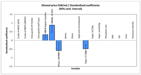
Figure 9.
Impacts of the significant variables on the European ethanol price. Source: Authors’ composition based on the price datasets.
The US ethanol prices changed in a different way compared to the European prices. Unlike in the EU, crude oil and conventional gasoline (NY Harbor) prices had a greater impact on the ethanol prices (Table 5). The negative impact of Gulf Coast conventional gasoline is surprising, but there is a complicated, nonlinear price fluctuation behind gasoline prices. Therefore, they do not necessarily move together [75]. Independence of the different energy markets was already proven in many cases, e.g., market decoupling between oil and gas in the US wholesale market [76]. There are many different reasons behind this, such as the composition of gasoline sales, different blending mandates, and/or tax differences. Regional price differences driven by the inventory stocks and refinery capacities can also be important [77]. As maize is the major raw material of the US ethanol production, it has a significant positive impact on the price of ethanol. Soft wheat did not turn out to be significant. However, hard wheat had the same, negative impact in the case of the US. Besides these variables, barley and urea were part of the models, and both had a negative impact on the ethanol prices.
Table 5.
Major influencing factors of US ethanol prices.
Regarding the MLR model with the COVID variable, the most spectacular result is the strong positive impact of the price of regular gasoline, while crude oil and conventional gasoline prices showed no impact on the price of US ethanol. In this model, the COVID-19 variable became significant with a strong negative impact on the ethanol prices, decreasing the monthly prices by USD 0.15 on average.
Using standardized coefficients, COVID-19 enlarged the price impact of maize as seen in Figure 10 and Figure 11. This is in line with our initial expectations. Another implication of the pandemic is the significant negative impact of hard wheat and barley prices on US ethanol prices.
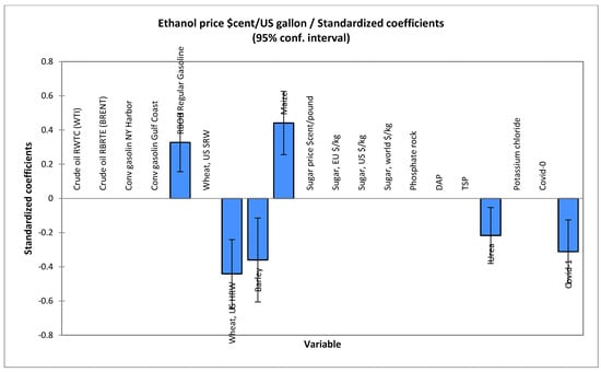
Figure 10.
Impacts of the significant variables on the ethanol price with COVID. Note: The blue bars show the average values, while their lines indicate the minimum/maximum intervals of the coefficients analyzed.
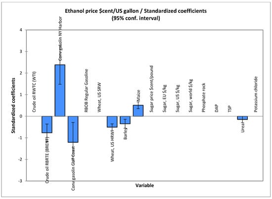
Figure 11.
Impacts of the significant variables on the ethanol price without COVID. Note: The blue bars show the average values, while their lines indicate the minimum/maximum intervals of the coefficients analyzed.
According to the facts, the pandemic hit the US more than the EU. Even though there is only a limited dataset available at this moment (the first 6 months of 2020), this impact could have been identified and proven by the regression and the two other models (MLR, MLR with COVID variable). This result is a supplement to Kim et al. (2020) [53], whose statements referred to the Asian and Pacific regions.
The major reason behind the different COVID-19 effects on these regional markets is their different characteristics. The US is not only the major consumer of oil and, via the mandatory blending mandate, ethanol, but also its major producer. COVID-19 resulted in lower mobility, which greatly decreased fuel consumption, as well as the production of fuel. The whole process was even amplified by the sharp depreciation of the US dollar against the euro at the end of February and the beginning of March [78]. This made US oil products cheaper for European consumers.
This drop of demand put the whole oil refinery sector under pressure with no significant alternatives for using the inventory of oil currently on hand. The high pressure on the storage capacity of oil led to a price of USD −37.63/barrel on 20 April 2020 [6]. As the EIA reported, US crude oil production was historically low in May, below the monthly production of the last 2.5 years [79]. They expect no significant increase in production in the close future, due to the difference between the lower production of the existing wells and the new drilling activities. Moreover, reduced vehicle use has a much higher impact on US consumption, as the fuel efficiency is historically lower in the US than in the EU [80].
4.3. Factor Analysis
The Kaiser-Meyer-Olkin Measure of Sampling Adequacy, Bartlett’s Test of Sphericity, and the correlation and anti-image correlation matrix verified that the confirmatory factor analysis (CFA) were carried out (Table 6).
Table 6.
Sampling adequacy for the factor analysis.
The final model consisted of four factors with oblimin rotation and 81.7% value of the Extraction Sums of Squared Loadings (Table 7).
Table 7.
Results of the factor analysis.
Based on the pattern matrix, we identified the following four factors:
- First factor: Crude oil and gasoline.
- Second factor: Raw materials (maize excluded).
- Third factor: Artificial fertilizers.
- Fourth factor: Maize.
These factors cover most of the initial variables except for urea and potassium chloride. Similar to the case of the individual variables, regression analysis was also carried out for the factors. According to our results, the European ethanol prices were driven by the third and fourth factors, while the US prices were determined by first, second, and fourth factors (Table 8).
Table 8.
Factor-based models of the ethanol prices.
These results are different from the previous, individual variable-based analysis. The factor-based analysis suggests that the major influencing factors of the European ethanol prices were the artificial fertilizers prices and maize prices (Figure 12), while the previous analysis was dominated by the wheat and sugar prices. This may be explained by the significant, but lower contribution of the maize and artificial fertilizers (or the higher contribution of the wheat and sugar) to the explanatory power of the individual regression model (Table 3). However, the COVID variable was not significant, even in the factor-based model. This strengthens our major findings, namely, the COVID-19 pandemic did not influence the European ethanol prices. These statements may be novel when compared to the currently known literature.
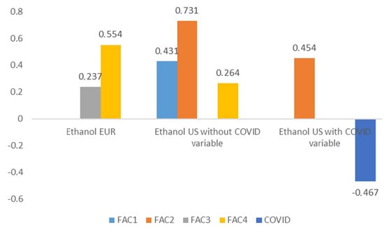
Figure 12.
Impacts of the different factors influencing ethanol prices. Source: Authors’ calculation.
Regarding the US ethanol prices, the factor-based results are similar to the previous, variable-based model. Fuel, raw materials, and maize prices became part of the influencing factors, corresponding with the results found by Elleby et al. (2020) [7]. The significance of the so-called COVID impact was also strengthened, as that variable affected the US ethanol prices. The factor-based model contained only raw materials and COVID as significant factors (Figure 12).
5. Conclusions
This study showed that there were significant differences between the US and EU ethanol prices, and that the gap between the price trends in each region is widening. These differences were highly dependent on the feedstock and on the structure of fuel consumption between the given regions. Consequently, the changes in ethanol prices in the two regions did not correlate with each other. Changes in fertilizer prices also had a statistically reliable effect on ethanol prices in several cases, but the trend and type of active ingredients also differed greatly between the two regions.
Based on the data available since the outbreak of COVID-19, the virus has reduced ethanol prices in the US, while it has had no measurable impact on the European ethanol market. The virus has also significantly reduced oil and phosphorus fertilizer prices but has had no effect on EU wheat prices. All of this may be related to typical consumer responses to the spread of the virus (less travel, food accumulation). In the US, the virus has significantly increased the price determinant role of maize.
Our factor analysis showed that the prices of sugar, maize, and competing final products (oil) influenced the ethanol prices in the US. These influencing factors were the prices of key raw materials and their inputs (corn, fertilizer) in the EU. COVID-19 did not change this in the EU, but in the US, the virus clearly excluded oil and maize from the price determinants of ethanol. Ethanol prices are expected to be greatly influenced by the spread of new generations of biofuels and the market of their feedstocks in the future.
Regarding the relationships between ethanol, oil, and maize prices, our results correspond with previous literature. However, the EU and US regional comparison and our major finding, that COVID-19 did not affect EU ethanol prices, can be considered novel.
The major limitation of the study is the small number of observations currently available. The price impacts of COVID-19 can be explained better when post-pandemic data are available. That would make it possible to evaluate the regional level price recovery process as well. Another future research path could be the use of further variables, such as competing energy products (e.g., natural gas or biodiesel) or other raw materials (e.g., soybean, sugar beet, or sorghum).
Author Contributions
Conceptualization, T.M. and A.B.; methodology, L.N.; software, L.N.; data curation, T.M., A.B. and Z.G.; investigation, results and conclusions, T.M. and A.B.; writing—original draft preparation, T.M., A.B. and Z.G.; writing—review and editing, T.M., A.B. and Z.G.; visualization, Z.G.; supervision, T.M. and A.B.; funding acquisition, T.M., A.B., Z.G. and L.N. All authors have read and agreed to the published version of the manuscript.
Funding
This research was supported by the National Research, Development and Innovation Office through the project Nr. 2019-1.3.1-KK-2019-00015, titled "Establishment of a circular economy-based sustainability competence center at the University of Pannonia" and the ÚNKP-20-4 New National Excellence Program of the Ministry for Innovation and Technology from the source of the National Research, Development and Innovation Fund.
Acknowledgments
The authors wish to thank Earl Ryan Kovacs for his edits and thorough proofreading.
Conflicts of Interest
The authors declare no conflict of interest.
References
- Allen, M.; Babiker, M.; Chen, Y.; de Coninck, H.; Connors, S.; van Diemen, R.; Zickfeld, K. Global Warming of 1.5 C: Special Report on the Impacts of Global Warming; Intergovernmental Panel on Climate Change (IPCC): Geneva, Switzerland, 2018. [Google Scholar]
- Meadows, D.; Randers, J.; Meadows, D. Limits to Growth: The 30-Year Update; Chelsea Green Publishing: White River Junction, VT, USA, 2004. [Google Scholar]
- Priyadarshini, P.; Abhilash, P.C. Circular economy practices within energy and waste management sectors of India: A meta-analysis. Bioresour. Technol. 2020, 304, 123018. [Google Scholar] [CrossRef] [PubMed]
- Németh, K.; Péter, E.; Szabó, P.; Pintér, G. Renewable energy alternatives in Central and Eastern European countries–through the example of Hungary. Georg. Agric. 2018, 24, 72–88. [Google Scholar]
- International Energy Agency (IEA). Renewables 2018. Market Analysis and Forecast from 2018 to 2023; International Energy Agency: Paris, France, 2018. [Google Scholar]
- Vaughan, L.; Chellel, K.; Bain, B. London Traders Hit $500 Million Jackpot When Oil Went Negative; Bloomberg Businessweek: Bloomberg, NY, USA, 2020. [Google Scholar]
- Elleby, C.; Domínguez, I.P.; Adenauer, M.; Genovese, G. Impacts of the COVID-19 Pandemic on the Global Agricultural Markets. Environ. Resour. Econ. 2020, 76, 1067–1079. [Google Scholar] [CrossRef] [PubMed]
- Bank, W. Most Commodity Prices to Drop in 2020 As Coronavirus Depresses Demand and Disrupts Supply; World Bank: Washington, DC, USA, 2020. [Google Scholar]
- International Energy Agency (IEA). Oil Market Report; International Energy Agency: Paris, France, 2017; p. 64. [Google Scholar]
- Bušić, A.; Kundas, S.; Morzak, G.; Belskaya, H.; Marđetko, N.; Ivančić Šantek, M.; Komes, D.; Novak, S.; Šantek, B. Recent trends in biodiesel and biogas production. Food Technol. Biotechnol. 2018, 56, 152–173. [Google Scholar] [CrossRef]
- Renewable Fuels Association (RFA). Ethanol Industry Outlook. Renewable Fuels Association. Powered with Renewed Energy; Renewable Fuels Association: Washington, DC, USA, 2019. [Google Scholar]
- BioEnergy2020+. BioEnergy2020+Database on Facilities for the Production of Advanced Liquid and Gaseous Biofuels for Transport. 2019. Available online: https://demoplants.bioenergy2020.eu/ (accessed on 20 June 2020).
- International Energy Agency (IEA). Biofuels for Transport; International Energy Agency: Paris, France, 2019. [Google Scholar]
- Stichnothe, H.; Meier, D.; de Bari, I. Biorefineries: Industry status and economics. In Developing the Global Bioeconomy; Elsevier: Amsterdam, The Netherlands, 2016; pp. 41–67. [Google Scholar]
- Sydney, E.B.; Letti, L.A.J.; Karp, S.G.; Sydney, A.C.N.; de Souza Vandenberghe, L.P.; de Carvalho, J.C.; Woiciechowski, A.L.; Medeiros, A.B.P.; Soccol, V.T.; Soccol, C.R. Current analysis and future perspective of reduction in worldwide greenhouse gases emissions by using first and second generation bioethanol in the transportation sector. Bioresour. Technol. Rep. 2019, 7, 100234. [Google Scholar] [CrossRef]
- Intelligence, M. Bio-Ethanol Market—Growth, Trends, and Forecast (2020–2025); Mordor Intelligence: Hyderabad, India, 2019. [Google Scholar]
- Niphadkar, S.; Bagade, P.; Ahmed, S. Bioethanol production: Insight into past, present and future perspectives. Biofuels 2018, 9, 229–238. [Google Scholar] [CrossRef]
- CARD. Historical Ethanol Operating Margins; Iowa State University, Center for Agricultural and Rural Development: Ames, IA, USA, 2020. [Google Scholar]
- Licht, F.O. World Ethanol & Biofuels Report; F.O. Licht: Brussels, Belgium, 2016. [Google Scholar]
- MarketsandMarkets. Bioethanol Market by Feedstock, End-use Industry, Fuel blend And Region—Global Forecast to 2025; MarketsandMarkets: Northbrook, IL, USA, 2020. [Google Scholar]
- Charles, C.; Gerasimchuk, I.; Bridle, R.; Moerenhout, T.; Asmelash, E.; Laan, T. Biofuels—At What Cost? A Review of Costs and Benefits of EU Biofuel Policies; The International Institute for Sustainable Development: Winnipeg, MB, Canada, 2013. [Google Scholar]
- Pacini, H.; Sanches-Pereira, A.; Durleva, M.; Kane, M.; Bhutani, A. The State of the Biofuels Market: Regulatory, Trade and Development Perspectives; United Nations: Geneva, Switzerland, 2014. [Google Scholar]
- Lane, J. Ethanol and Biodiesel: Dropping below the Production Cost of Fossil Fuels? 2017. Available online: https://www.biofuelsdigest.com/bdigest/2017/05/18/ethanol-and-biodiesel-dropping-below-the-production-cost-of-fossil-fuels/ (accessed on 18 June 2020).
- Mizik, T. Impacts of International Commodity Trade on Conventional Biofuels Production. Sustainability 2020, 12, 2626. [Google Scholar] [CrossRef]
- de Wit, M.P.; Faaij, A.P.C. Biomass Resources Potential and Related Costs. Assessment of the EU-27, Switzerland, Norway and Ukraine; Copernicus Institute–Utrecht University: Utrecht, The Netherlands, 2008. [Google Scholar]
- Saini, S.; Chandel, A.K.; Sharma, K.K. Past practices and current trends in recovery and purification of first generation ethanol: A learning curve for lignocellulosic ethanol. J. Clean. Prod. 2020, 268, 122357. [Google Scholar] [CrossRef]
- Platts Europe. Platts Europe Company Data. 2020. Available online: https://www.spglobal.com/platts/en/products-services/electric-power/power-in-europe (accessed on 23 June 2020).
- Qin, Y.; Hong, K.; Chen, J.; Zhang, Z. Asymmetric effects of geopolitical risks on energy returns and volatility under different market conditions. Energy Econ. 2020, 90, 104851. [Google Scholar] [CrossRef]
- Garside, M. Oil—Global Production 1998–2019; Statista: New York, NY, USA, 2020. [Google Scholar]
- International Energy Agency (IEA). Oil Market Report; International Energy Agency: Paris, France, 2020. [Google Scholar]
- Sönnichsen, N. Coronavirus: Impact on the Global Energy Industry—Statistics & Facts. Statista.com. 2020. Available online: https://www.statista.com/topics/6254/coronavirus-covid-19-impact-on-the-energy-industry/ (accessed on 15 September 2020).
- Van der Ploeg, F. Natural resources: Curse or blessing? J. Econ. Lit. 2011, 49, 366–420. [Google Scholar] [CrossRef]
- Majumder, M.K.; Raghavan, M.; Vespignani, J. Oil curse, economic growth and trade openness. Energy Econ. 2020, 91, 104896. [Google Scholar] [CrossRef]
- Alghalith, M. The interaction between food prices and oil prices. Energy Econ. 2010, 32, 1520–1522. [Google Scholar] [CrossRef]
- Nazlioglu, S. World oil and agricultural commodity prices: Evidence from nonlinear causality. Energy Policy 2011, 39, 2935–2943. [Google Scholar] [CrossRef]
- Prakash, A. Organisation des Nations Unies Pour L’alimentation et L’agriculture. In Safeguarding Food Security in Volatile Global Markets; Food and Agriculture Organization of the United Nations: Rome, Italy, 2011; p. 38. [Google Scholar]
- Trujillo-Barrera, A.; Mallory, M.; Garcia, P. Volatility spillovers in US crude oil, ethanol, and corn futures markets. J. Agric. Resour. Econ. 2012, 37, 247–262. [Google Scholar]
- Natanelov, V.; McKenzie, A.M.; Van Huylenbroeck, G. Crude oil–corn–ethanol–nexus: A contextual approach. Energy Policy 2013, 63, 504–513. [Google Scholar] [CrossRef]
- Dong, Z. Does the Development of Bioenergy Exacerbate the Price Increase of Maize? Sustainability 2019, 11, 4845. [Google Scholar] [CrossRef]
- Bahel, E.; Marrouch, W.; Gaudet, G. The economics of oil, biofuel and food commodities. Resour. Energy Econ. 2013, 35, 599–617. [Google Scholar] [CrossRef]
- OECD-FAO. Agricultural Outlook 2019–2028. Chapter 9. Biofuels; Organisation for Economic Co-operation and Development: Paris, France, 2019. [Google Scholar]
- Manochio, C.; Andrade, B.; Rodriguez, R.; Moraes, B. Ethanol from biomass: A comparative overview. Renew. Sustain. Energy Rev. 2017, 80, 743–755. [Google Scholar] [CrossRef]
- Adjesiwor, A.T.; Islam, M.A. Rising nitrogen fertilizer prices and projected increase in maize ethanol production: The future of forage production and the potential of legumes in forage production systems. Grassl. Sci. 2016, 62, 203–212. [Google Scholar] [CrossRef]
- Ott, H. Fertilizer Markets and Their Interplay with Commodity and Food Prices; EUR 25392 EN Joint Research Centre: Brussels, Belgium, 2012; p. 36. [Google Scholar]
- Mojović, L.; Pejin, D.; Grujić, O.; Markov, S.; Pejin, J.; Rakin, M.; Vukašinović, M.; Nikolić, S.; Savić, D. Progress in the production of bioethanol on starch-based feedstocks. Chem. Ind. Chem. Eng. Q. CICEQ 2009, 15, 211–226. [Google Scholar] [CrossRef]
- United States Department of Agriculture (USDA). World Agricultural Production; United States Department of Agriculture, Foreign Agricultural Service: Washington, DC, USA, 2020; p. 42. [Google Scholar]
- Food and Agriculture Organization of the United Nations (FAO). Faostat—Crops; Food and Agriculture Organization of the United Nations: Rome, Italy, 2020. [Google Scholar]
- USDE. Maps and Data—Corn Production and Portion Used for Fuel Ethanol; U.S. Department of Energy, Energy Efficiency & Renewable Energy, Alternative Fuels Data Center: Washington, DC, USA, 2020.
- de Oliveira Bordonal, R.; Carvalho, J.L.N.; Lal, R.; de Figueiredo, E.B.; de Oliveira, B.G.; La Scala, N. Sustainability of sugarcane production in Brazil. A review. Agron. Sustain. Dev. 2018, 38, 13. [Google Scholar] [CrossRef]
- Economic Research Division Data (FRED). Graph Observations, Federal Reserve Economic Data; Economic Research Division, Federal Reserve Bank of St. Louis: St. Louis, MO, USA, 2020. [Google Scholar]
- Energy Information Administration (EIA). Short-Term Energy Outlook; Energy Information Administration—Official Energy Statistics from the U.S. Government: Washington, DC, USA, 2020. [Google Scholar]
- Bassols, A.; Bassols, F. The Oil Industry and Its Relation to the Pandemic COVID 19. Arch. Pet. Env. Biotech. Nol. 2020, 5, 164. [Google Scholar]
- Kim, K.; Kim, S.; Park, C.-Y. Food Security in Asia and the Pacific Amid the COVID-19 Pandemic. 2020. Available online: https://www.adb.org/publications/food-security-asia-pacific-covid-19 (accessed on 7 July 2020).
- Hart, C.; Hayes, D.J.; Jacobs, K.L.; Schulz, L.L.; Crespi, J. The Impact of COVID-19 on Iowa’s Corn, Soybean, Ethanol, Pork, and Beef Sectors. 2020. Available online: https://lib.dr.iastate.edu/card_policybriefs/30/ (accessed on 8 July 2020).
- Shruthi, M.; Ramani, D. Statistical analysis of impact of COVID 19 on India commodity markets. Mater. Today Proc. 2020. [Google Scholar] [CrossRef] [PubMed]
- Barichello, R. The COVID-19 pandemic: Anticipating its effects on Canada’s agricultural trade. Can. J. Agric. Econ. Rev. Can. D Agroecon. 2020. [Google Scholar] [CrossRef]
- Lucas, B. Impacts of Covid-19 on Inclusive Economic Growth in Middle-Income Countries; K4D Helpdesk Report 811; Institute of Development Studies: Brighton, UK, 2020; p. 32. [Google Scholar]
- Shretta, R. The Economic Impact of COVID-19; Centre for Tropical Medicine and Global Health, Nuffield Department of Medicine, University of Oxford: Oxford, UK, 2020. [Google Scholar]
- WTO. Trade Set to Plunge as COVID-19 Pandemic Upends Global Economy. 2020. Available online: https://www.wto.org/english/news_e/pres20_e/pr855_e.htm (accessed on 10 July 2020).
- Sperling, F.; Havlik, P.; Denis, M.; Gaupp, F.; Palazzo, A.; Valin, H.; Visconti, P. Report on Second Consultative Science Platform. Bouncing Forward Sustainably: Pathways to a post-COVID World. Resilient Food Systems. 2020. Available online: http://pure.iiasa.ac.at/id/eprint/16657/ (accessed on 10 July 2020).
- Subhash, V.; Sapre, A.; Dasgupta, S. Possible Prevention of COVID 19 by Using Linoleic Acid (C18) Rich Algae Oil. AIJR Prepr. 2020. [Google Scholar] [CrossRef]
- Agrawal, A.; Prajapati, H.; Shukla, P.; Gupta, A.K. Jatropha curcus plant as Antiviral agent and as a Biodiesel. Int. J. Pharm. Life Sci. 2020, 11, 6516–6519. [Google Scholar]
- Black, W.; Babin, B.J. Multivariate data analysis: Its approach, evolution, and impact. In The Great Facilitator; Babin, B., Sarstedt, M., Eds.; Springer: Cham, Switzerland, 2019; pp. 121–130. [Google Scholar]
- Ge, Y.; Wu, H. Prediction of corn price fluctuation based on multiple linear regression analysis model under big data. Neural Comput. Appl. 2019, 32, 16843–16855. [Google Scholar] [CrossRef]
- Ciulla, G.; D’Amico, A. Building energy performance forecasting: A multiple linear regression approach. Appl. Energy 2019, 253, 113500. [Google Scholar] [CrossRef]
- Miao, R. Impact of ethanol plants on local land use change. Agric. Resour. Econ. Rev. 2013, 42, 291–309. [Google Scholar] [CrossRef]
- Koop, G. Analysis of Economic Data; OSIRIS Publishing House: Budapest, Hungary, 2008. [Google Scholar]
- Hair, J.; Black, W.; Babin, B.; Anderson, R. Multivariate Data Analysis, 7th ed.; Pearson Education Limited, Pearson Prentice Hall: London, UK, 2009. [Google Scholar]
- Esmaeili, A.; Shokoohi, Z. Assessing the effect of oil price on world food prices: Application of principal component analysis. Energy Policy 2011, 39, 1022–1025. [Google Scholar] [CrossRef]
- Suhr, D.D. Principal Component Analysis vs. Exploratory Factor Analysis (Paper 203-30). In Proceedings of the Thirtieth Annual SAS® Users Group International Conference, Philadelphia, PA, USA, 10–13 April 2005; p. 30. [Google Scholar]
- Meglen, R.R. Examining large databases: A chemometric approach using principal component analysis. J. Chemom. 1991, 5, 163–179. [Google Scholar] [CrossRef]
- Energy Information Administration (EIA). Petroleum & Other Liquids. In Release Date; U.S. Energy Information Administration: Washington, DC, USA, 2020. [Google Scholar]
- Bank, W. World Bank Commodities Price Data (The Pink Sheet); World Bank: Washington, DC, USA, 2020. [Google Scholar]
- McFadden, D. Econometric models for probabilistic choice. In Structural Analysis of Discrete Data with Econometric Applications; Manski, C., McFadden, D., Eds.; MIT Press: Cambridge, MA, USA, 1981. [Google Scholar]
- Zhang, G.; Tian, L.; Zhang, W.; Yan, X.; Wan, B.; Zhen, Z. A Study on the Similarities and Differences of the Conventional Gasoline Spot Price Fluctuation Network between Different Harbors. Sustainability 2020, 12, 710. [Google Scholar] [CrossRef]
- Perifanis, T.; Dagoumas, A. Price and volatility spillovers between the US crude oil and natural gas wholesale markets. Energies 2018, 11, 2757. [Google Scholar] [CrossRef]
- Kumar, D.K.; Renshaw, J. Gasoline Flows away from New York Harbor as Midwest Prices Soar. 2017. Available online: https://fr.reuters.com/article/us-usa-gasoline-new-york-idUSKBN1D02V3 (accessed on 20 July 2020).
- ECB. Euro Reference Exchange Rates; European Central Bank: Frankfurt, Fermany, 2020. [Google Scholar]
- EIA. Short-Term Energy Outlook; U.S. Energy Information Administration: Washington, DC, USA, 2020. [Google Scholar]
- An, F.; Sauer, A. Comparison of passenger vehicle fuel economy and greenhouse gas emission standards around the world. Pew Cent. Glob. Clim. Chang. 2004, 25. Available online: https://www.c2es.org/site/assets/uploads/2004/12/comparison-passenger-vehicle-fuel-economy-ghg-emission-standards-around-world.pdf (accessed on 21 July 2020).


Publisher’s Note: MDPI stays neutral with regard to jurisdictional claims in published maps and institutional affiliations. |
© 2020 by the authors. Licensee MDPI, Basel, Switzerland. This article is an open access article distributed under the terms and conditions of the Creative Commons Attribution (CC BY) license (http://creativecommons.org/licenses/by/4.0/).