Energy-Efficient Autonomous Navigation of Solar-Powered UAVs for Surveillance of Mobile Ground Targets in Urban Environments

Abstract

In this paper, we consider the navigation of a group of solar-powered unmanned aerial vehicles (UAVs) for periodical monitoring of a set of mobile ground targets in urban environments. We consider the scenario where the number of targets is larger than that of the UAVs, and the targets spread in the environment, so that the UAVs need to carry out a periodical surveillance. The existence of tall buildings in urban environments brings new challenges to the periodical surveillance mission. They may not only block the Line-of-Sight (LoS) between a UAV and a target, but also create some shadow region, so that the surveillance may become invalid, and the UAV may not be able to harvest energy from the sun. The periodical surveillance problem is formulated as an optimization problem to minimize the target revisit time while accounting for the impact of the urban environment. A nearest neighbour based navigation method is proposed to guide the movements of the UAVs. Moreover, we adopt a partitioning scheme to group targets for the purpose of narrowing UAVs’ moving space, which further reduces the target revisit time. The effectiveness of the proposed method is verified via computer simulations.

1. Introduction

Unmanned aerial vehicles (UAVs) have found numerous applications in both military and civilian domains. They are excellent tools for target surveillance and monitoring [1,2,3], thanks to their flexibility. Because using a single UAV is often inefficient to conduct a complex mission, employing a UAV team is the trend in order to complete missions quickly [4]. When multiple UAVs conduct some missions, they are often regarded as a multiagent system. In the past few decades, the coordination issue of multiagent systems has attracted great attention from different research communities [5,6,7].

This paper pays attention to the moving target surveillance by a group of UAVs. A practical application of the considered scenario is that, in wireless sensor networks, the sensor nodes collect data from the environment. UAVs function as data sinks to collect the sensory data from sensor nodes [8]. In general, the number of available UAVs is smaller than that of the sensor nodes. Thus, the UAVs carry out a periodical surveillance of the sensor nodes.

Because UAVs often have limited onboard battery capacity, their operation duration is constrained. Installing solar-panels enables the UAVs to harvest energy from the sun, which is promising for prolonging the lifetime of the UAVs in the sunny daytime [9]. We consider the surveillance of mobile targets by the solar-powered UAVs in urban environments. The tall buildings have some negative impact on the mission. Firstly, they may create some shadow region, where the Line-of-Sight (LoS) between the UAVs and the sun is blocked, so that the UAVs cannot harvest energy if they fly in the shadow region. Besides, the buildings may also block the LoS between the UAVs and considered targets. This may prevent a UAV from successfully surveying a target.

The problem of interest is formulated as an optimization problem to minimize the target revisit time by planning the UAVs’ paths. To address the problem, we present a path planning method that is based on the Rapidly-exploring Random Tree (RRT). This method can quickly find a feasible path for the UAV to intercept the target in the scenario where the target moves along a known trajectory. We then consider the case with one UAV and multiple targets. We present a nearest neighbour (NN) based navigation method. The so-called NN involves both the UAV-target distance as well as the uncertainty level of a target. Finally, we consider the multi-UAV and multi-target case. We partition the targets into groups according to the distance information between the targets and the UAVs. Subsequently, each UAV takes care of the targets in its own partition.

The proposed autonomous navigation algorithm that navigates a UAV team in order to periodically survey a group of mobile ground targets is the main contribution of this paper. It is computationally efficient and easily implementable online, since it is a randomized RRT-based approach. Extensive simulation results are reported in order to confirm the effectiveness of the developed method.

The reminder of the paper is organized, as follows. Section 2 briefly reviews the relevant work. Section 3 presents the system models and formulates the problem. Section 4 presents the proposed UAV navigation approaches. Section 5 reports the computer simulation results, and Section 6 gives the concluding remarks.

2. Related Work

The target surveillance problem that is considered in this paper has not been considered in any existing publications. In this section, we present some closely relevant publications, so that we can distinguish the contributions of the paper with others.

The target surveillance problem has been investigated from different levels in the literature. In terms of sensing, a large number of image/video processing strategies have been developed in order to estimate states of the targets from the measured images/videos [10,11,12,13,14]. In these publications, attention has been paid to the quality of detection for a single target.

In the scenario with multiple targets, how to allocate the UAV resource becomes necessary to achieve a good quality of surveillance. Many operational research results, such as the conventional travelling salesman problem (TSP) [15] and the vehicle routing problem (VRP) [16], are the common tools for planning the UAVs’ paths. When there are enough UAVs, the coverage control has been investigated to achieve the optimal sensing coverage of the targets [17,18]. In cases where moving targets are to be monitored, and to maintain the quality of sensing, the reactive algorithms have been proposed [2,19].

This paper focuses on the scenario where the number of UAVs is not enough to persistently monitor the targets, so a periodical surveillance is conducted by the UAVs. As the targets are moving in the considered region, the problem is more relevant to the time-dependent TSP [20] and the moving-target TSP [21,22]. In the time-dependent TSP [20], the common setting is to find the shortest tour for the salesman in a graph with time-dependent edges. In the moving-target TSP [21,22], the targets are assumed to move with a constant speed along a fixed direction. The problem considered here is different from them. Firstly, the targets move along some trajectories, so that their speeds and moving directions may change with time. Secondly, the existence of buildings in the urban environment requires the UAVs to avoid collision with the buildings. Thirdly, the UAVs need to harvest energy from the sun to enable the UAVs to operate in the given time period. However, each path depends on the UAV’s initial position, the buildings’ positions and the target’s trajectory, which is challenging to be known in advance. Thus, both the moving-target TSP and the time-dependent TSP cannot be applied to address the problem that is considered in the paper.

Path planning plays an important role in this work. Among various path planning algorithms, RRT is a sampling-based approach. It generates a feasible (but may not be optimal) path quickly, even if the environment is complicated. Many publications have reported that this method can be easily applied in real-time applications, such as mobile ground robots [23] and autonomous driving [24]. To improve the solution quality and computing speed, many RRT variants have been developed. Specific attention has been paid to the generation of samples and the control of the searching step length. A lower bound tree-RRT is designed to find out the near optimal path [25]. Besides, a node control strategy is proposed in order to restrict the expansion of the random tree [26]. Because of the computational efficiency, RRT-based approaches are generally suitable to run in real-time, and it also has potential to be implemented in a decentralized manner [27]. We adopt the RRT approach in this paper. However, as will be shown in the following sections, we do not have a fixed destination for a UAV. Instead, the destination of a UAV moves. Our objective is generate a feasible path in real-time, so that the UAV can intercept the target as soon as possible.

3. System Model and Problem Statement

Suppose that we have a team of solar-powered UAVs labelled $1,2,\dots ,I$. We consider that these solar-powered UAVs fly at a fixed altitude z in an urban area to conduct some missions. For UAV i, let $p_i\left(t\right)=[x_i\left(t\right),y_i\left(t\right),z]$ be its position in the ground frame at t, ${\theta }_i\left(t\right)$ be the horizontal heading angle with respect to the x-axis; and, $v_i\left(t\right)$ and ${\omega }_i\left(t\right)$ be its linear and angular speeds, respectively. The motion of UAV i can be described by the following equations [28,29]:

$$\begin{array}{c}\hfill \left\{\begin{array}{c}{\dot{x}}_i\left(t\right)=v_i\left(t\right)cos\left({\theta }_i\left(t\right)\right),\hfill \\ {\dot{y}}_i\left(t\right)=v_i\left(t\right)sin\left({\theta }_i\left(t\right)\right),\hfill \\ {\dot{\theta }}_i\left(t\right)=w_i\left(t\right),\hfill \end{array}\right.\end{array}$$

(1)

In this paper, the effect of wind has not been considered. The following constraints hold for any UAV at any time:

$$\begin{array}{c}\hfill \left\{\begin{array}{c}-V_i^{\max }\le v_i\left(t\right)\le V_i^{\max },\hfill \\ -{\Omega }_i^{\max }\le w_i\left(t\right)\le {\Omega }_i^{\max },\hfill \\ (x_i\left(t\right),y_i\left(t\right))\in \mathcal{D},\hfill \end{array}\right.\end{array}$$

(2)

Here, ${\Omega }_i^{max}$ and $V_i^{max}$ are the given constants, and $\mathcal{D}\subset {\mathbf{R}}^2$ is the considered area. The movement of many UAVs can be described by (1) and (2); see [30,31,32,33]. It is worth pointing out that, in (2), the linear speed $v_i\left(t\right)$ can take a negative value. This allows for a UAV to move backward when necessary. In Section 5, we will see some UAV trajectories with sharp turns, and the reason is that a negative linear speed is applied. This avoids making a large turn by moving along a circle.

Table 1. Symbols and meanings.

Symbol	Meaning
$p_i\left(t\right)$	UAV i’s position at time t
${\theta }_i\left(t\right)$	UAV i’s heading angle
$v_i\left(t\right)$	UAV i’s linear speed
${\omega }_i\left(t\right)$	UAV i’s angular speed
$\alpha$	Observation angle
R	Radius of the vision cone
$P_i\left(t\right)$	UAV i’s consuming power
$P_i^{sun}\left(t\right)$	UAV i’s harvesting power
$Q_i\left(t\right)$	UAV i’s residual energy
$q_i\left(t\right)$	Target j’s position
${\tau }_j$	Target j’s revisit time
$d_{ij}\left(t\right)$	Horizontal distance between UAV i and target j

summarizes the frequently used symbols in the paper, together with their meanings.

Let $P_i^{sun}\left(t\right)$ be the harvesting power of the solar energy. It can be computed as follows [34]

$$P_i^{sun}\left(t\right)=\eta A_{i}cos\varphi \left(t\right),$$

(3)

where $\eta$ represents the solar cell efficiency, $A_i$ represents the area of the solar cells, and $\varphi$ gives the incidence angle. The incidence angle $\varphi$ is further dependent on the azimuth angle ${\alpha }_z$ and the elevation angle ${\alpha }_e$ of the sun, and in the day time, both ${\alpha }_z$ and ${\alpha }_e$ vary with time.

The UAVs consume energy when they are flying. For the energy consuming power, we follow the model that was used in [35]:

$$P_i\left(t\right)={\lambda }_0\left(1+\frac{3v_i^2}{U_{tip}^2}\right)+\frac{1}{2}\rho \kappa sS{v}_i^3\left(t\right)+{\lambda }_1{\left(\sqrt{1+\frac{v_i^4\left(t\right)}{4{\mu }^4}}-\frac{v_i^2\left(t\right)}{2{\mu }^2}\right)}^{\frac{1}{2}},$$

(4)

where ${\lambda }_0$, ${\lambda }_1$ and $\mu$ are the blade profile power, the induced power and the mean rotor induced velocity in hovering, respectively; $U_{tip}$ represents the tip speed of the rotor blade; $\kappa$ is the fuselage drag ratio; s represents the rotor solidity; $\rho$ is the air density; and, $S_i$ rotor disc area.

Let $Q_i\left(t\right)$ denote the residual energy of the battery of UAV i. We have

$${\dot{Q}}_i\left(t\right)=P_i^{sun}\left(t\right)-P_i\left(t\right).$$

(5)

Moreover, $Q_i^{max}$ represents the upper bound of $Q_i\left(t\right)$.

Each UAV carries a ground-facing camera, and the camera’s observation angle is denoted by $\alpha \in (0,\pi )$; see Figure 1. If a target locates in a disc centred at $p_i\left(t\right)$ of the radius

$$R=ztan\left(\frac{\alpha }{2}\right),$$

(6)

and has LoS with the UAV, it can be observed by the UAV. We assume that a gimble is available on the UAV, so that, no matter how the UAV moves, the camera always faces the ground.

Now, we model the buildings. In this paper, each building is modelled as the smallest prism to enclose this building. Each prism has two parallel and congruent bases and a number of flat sides that are perpendicular to the $xy$-plane; see Figure 2. Each prism is characterized: $\Psi$, $\psi$ and h. $\Psi$ is a $\kappa$-by-2 matrix and $\psi$ is a $\kappa$-by-one vector. They determine the shape and size of the base. h is a scalar indicating the height of the prism. For a point $(x,y,z)$, if it is inside a prism, (7) holds:

$$\begin{array}{c}\hfill \left\{\begin{array}{c}\Psi \left[\begin{array}{c}x\\ y\end{array}\right]\le \psi ,\hfill \\ 0\le z\le h.\hfill \end{array}\right.\end{array}$$

(7)

Given the environment information, $\Psi$, $\psi$ and h are known for each building. Subsequently, we can have a subset of space, denoted by ${\mathcal{X}}_{building}$, which corresponds to these buildings. At any time, the UAVs must not be inside ${\mathcal{X}}_{building}$. Clearly, avoiding ${\mathcal{X}}_{building}$ is similar to the collision avoidance with steady obstacles [36,37].

Having the model of buildings is not sufficient to characterize the observation region of a UAV. We also need a method to determine whether a position in the air and a position on the ground have LoS. For this purpose, we consider the straight line segment between two points p and q, which is described as

$$\begin{array}{c}\hfill \left\{\begin{array}{c}x=x_q+{\beta }_x\tau ,\hfill \\ y=y_q+{\beta }_y\tau ,\hfill \\ z=z_q+{\beta }_z\tau ,\hfill \\ min\{x_p,x_q\}\le x_q+\alpha \tau \le max\{x_p,x_q\},\hfill \end{array}\right.\end{array}$$

(8)

where $q=(x_q,y_q,z_q)$, $p=(x_p,y_p,z_p)$, $({\beta }_x,{\beta }_y,{\beta }_z)=\frac{\overrightarrow{pq}}{\parallel \overrightarrow{pq}\parallel }$, and $\tau$ is a free variable.

Whether p and q have LoS can be tested by looking for the intersection points between the the line segment connecting p and q (8) and any prism (7). Because the environment information is known, whether p and q have LoS can be easily confirmed. We introduce a function $LOS(p,q,{\mathcal{X}}_{building})$:

$$LOS(p,q,{\mathcal{X}}_{building})=\left\{\begin{array}{c}\begin{array}{c}1,\mathrm{if}p\mathrm{and}q\mathrm{have}\mathrm{LoS},\hfill \\ 0,\mathrm{otherwise}.\hfill \end{array}\hfill \end{array}\right.$$

(9)

With this function, we can also test whether a UAV and the sun have LoS. To this end, the sun’s location needs to be known. Let V, a unit vector, denote the sunlight direction. With V, we can imagine that the sun is at $q_{sun}=p-V\tau$, where the parameter $\tau$ takes a large value so that the sun is far from the point p. We need to place the sun at a relatively far position. The reason is that we use the line segment to verify whether two points have LoS. When the sun is placed closely to the point p, we may not obtain the correct verification.

Let $b_i\left(t\right)$ be a binary variable indicating whether UAV i has LoS with the sun. Subsequently, UAV i’s residual energy can be computed by:

$${\dot{Q}}_i\left(t\right)=P_i^{sun}\left(t\right)b_i\left(t\right)-P_i\left(t\right).$$

(10)

There are N ground mobile targets in the given urban environment to be periodically surveyed. These targets can be some sensor nodes to measure the environment information of interest. Instead of continuously transmitting the sensory data, they only upload their sensory data to a control unit via the UAVs in proximity. This setting can prolong the lifetime of the nodes when the sensory data are of large size, such as videos. We assume that the UAVs know the current positions of the targets, and this information can be provided by the targets, since the energy consumption of reporting the position information can be ignored compared to the large size of sensory data. We also assume that the targets’ future positions are predictable. This assumption is reasonable, since, when the targets carry out some pre-defined missions, their trajectories can be known. Let $q_j\left(t\right)\in {\mathbf{R}}^3$ denote target j’s location ($j=1,\dots ,N$) at time t.

In this paper, we consider that $I<N$ and the targets spread in the considered environment. Subsequently, there may be some time in which a target is not under surveillance. From the common sense, the uncertainty level of a target relates to the time in which it is not under surveillance. Thus, a significant objective of the surveillance system is to maintain the uncertainty level of the targets as low as possible. This can be formulated as the minimization of the maximum target revisit time. Let ${\tau }_j$ denote the time gap between two consecutive visits of target j. Let $d_{ij}\left(t\right)$ denote the horizontal distance between target j and UAV i at time t.

Definition 1.

Target j is under surveillance of UAV i at time t, if $LOS(p_i\left(t\right),q_j\left(t\right),{\mathcal{X}}_{building})=1$ and $d_{ij}\left(t\right)\le R$.

Let $s_j\left(t\right)$ be a binary variable indicating if target j is under surveillance at time t. Subsequently, we have

$$s_j\left(t\right)=\left\{\begin{array}{c}\begin{array}{c}1,\mathrm{if}\exists i\mathrm{such}\mathrm{that}LOS(p_i\left(t\right),q_j\left(t\right),{\mathcal{X}}_{building})=1\mathrm{and}{d}_{ij}\left(t\right)\le R,\hfill \\ 0,\mathrm{otherwise}.\hfill \end{array}\hfill \end{array}\right.$$

(11)

Afterwards, we can use $s_j\left(t\right)$ to calculate ${\tau }_j$. Specifically, we have

$${\tau }_j=\underset{s_j\left(t_1\right)=1,s_j\left(t_2\right)=1,t_1<t_2,\forall t_1<t<t_2,s_j\left(t\right)=0}{max}{t}_2-t_1.$$

(12)

In other words, ${\tau }_j$ is the time instant gap between the two consecutive visits. Note that, if there is only one visit during the mission period $[0,T]$, i.e., at $t_1$, then, ${\tau }_j=T-t_1$. If there is not any visit during the mission period, then ${\tau }_j=T$.

The problem under investigation is to develop a navigation method for the UAVs modelled by (1) and (2) in order to minimize the maximum revisit time during the mission period $[0,T]$, i.e.,

$$min\underset{j=1,\dots ,N}{max}{\tau }_j.$$

(13)

subject to

$$Q_i\left(t\right)>0,\forall i,\forall t\in [0,T].$$

(14)

The problem under consideration is difficult to address optimally. Although we can have the trajectories of targets and predict their positions for the period of $[0,T]$, it is still hard to plan the trajectories of the UAVs in advance. The main reason lies in the complexity of the flying space in urban environments. In particular, due to the existence of buildings, the trajectory of UAV i (suppose that it is assigned to survey target j) depends on both the trajectory of target j and the position of UAV i at which it is assigned with this task. Furthermore, the UAV’s position depends on its last task. The coupling of the high-level task assignment problem and the low-level trajectory planning problem makes it too complex to be addressed optimally. Even if an optimal solution can be obtained, it may also take so long time that it cannot be applied online.

4. Proposed Navigation Method

4.1. Lifetime of UAVs

Before presenting the navigation method, it is necessary to discuss the lifetime of the UAVs. As shown in (3), for a UAV, its energy harvesting power varies with time because of the movement of the sun. Subsequently, the maximum harvested energy amount by UAV i is given by ${\int }_0^T\eta A_{i}cos\varphi \left(t\right)dt$.

According to (4), the energy consuming power $P_i$ increases with the speed $v_i$ in the first and second terms, while decreases with $v_i$ in the third term. Additionally, the third term weights more when $v_i$ is relatively small, while the first and second terms weight more when $v_i$ is relatively large. Thus, the energy consuming power $P_i$ in (4) first decreases and then increases with $v_i$. Figure 3 shows an illustrative plot of the relationship between $P_i$ and $v_i$. There exists an optimal linear speed, such that the energy consuming power is minimized. Let $P_i^{opt}$ denote the minimum energy consuming power.

We assume that $Q_i^{max}$ is the initial energy of UAV i. The necessary condition for the UAV to conduct the surveillance mission is as follows:

$$Q_i^{max}+{\int }_0^T\eta A_{i}cos\varphi \left(t\right)dt-T{P}_i^{opt}>0.$$

(15)

Once (15) holds, the UAV can complete the surveillance mission with the optimal linear speed, although this does not guarantee the performance of surveillance. Moreover, a hidden assumption of (15) is that the UAV always has LoS with the sun in $[0,T]$. Otherwise, the harvested energy amount is smaller than ${\int }_0^T\eta A_{i}cos\varphi \left(t\right)dt$. However, if (15) does not hold, the UAV cannot conduct the mission. If the capacity $Q_i^{max}$ takes some larger value, it is allowed to have some part of the UAV trajectory having no LoS with sun. The margin of capacity has the potential to reduce the revisit time. There are two feasible paths for the UAV to intercept the target, as shown in Figure 4. The red one has some part behind the building that prevents the UAV from harvesting energy, while the green path enables the UAV to harvest energy during the trip. The red one leads to a shorter time for the UAV to survey the target than the green. If there is no margin capacity, then the UAV has to follow the green path. Otherwise, it can follow the red one to reduce the revisit time.

Though the margin energy capacity brings benefit in terms of the reduction of the revisit time, it also creates challenges in the management of this amount of energy. Specifically, the UAV may need to survey several targets during the mission. Subsequently, it is difficult to decide how to allocate the margin capacity to the tasks. In the subsequent parts, we assume that there is no such margin capacity, and the UAVs fly at their corresponding optimal linear speeds. Accordingly, the UAVs always look for paths having LoS with sun. We leave the complex case with margin capacity for future study.

4.2. One UAV and One Target

In the simplest case, we consider that one UAV is assigned to survey a target. Suppose that it is at $t_0$ the UAV starts to move to the target. We denote the initial positions of the UAV and the target as $p\left(t_0\right)$ and $q\left(t_0\right)$, respectively, and the initial heading angle of the UAV as $\theta \left(t_0\right)$. We use $\mathbf{x}\left(t\right)=\left[p\right(t),\theta (t\left)\right]$ to represent the state of the UAV. Suppose we know the trajectory of the target in the considered area $\mathcal{D}$, and we make a prediction for its future positions in the time interval $[t_0,t_0+T_0]$. Formally, we know $q\left(t\right)$, where $t\in [t_0,t_0+T_0]$. We select a suitable $T_0$, so that the UAV can intercept the target before $t_0+T_0$.

For the purpose of implementing the method online, we adopt the computationally efficient RRT approach. The common setting of the RRT approach looks for a feasible path between a start position and a destination, and the obtained path can avoid obstacles. In our problem, the buildings that are taller than the UAV flying altitude are regarded obstacles. Our problem has some additional features compared to the common setting. Firstly, different from a stationary destination, the destination in our problem, i.e., the target, is moving. Secondly, the UAV should avoid shadow region, because it needs to always harvest energy during the trip.

The objective is to find a feasible UAV path, such that, at time instant $t\in [t_0,t_0+T_0]$, the target locates inside the vision cone of the UAV and they have LoS. Starting from the current UAV position, i.e., $p\left(t_0\right)$, we generate a random tree. The termination condition of the tree generation process is that $d\left(t\right)\le R$ and $LOS(p\left(t\right),q\left(t\right),{\mathcal{X}}_{building})=1$ at time t, where $d\left(t\right)$ is the horizontal UAV-target distance.

We present all of the procedures in Algorithm 1. Let $\mathcal{T}$ denote the random tree and $\delta$ be a sampling interval. $\mathcal{T}$ consists of a set of vertices. A vertex is annotated with control inputs, parent vertex and timestamp. Firstly, we initialize the tree $\mathcal{T}$ with $\mathbf{x}\left(t_0\right)$. Subsquently, we keep generating random samples in the space, find the nearest vertex from the tree to the sample, choose the suitable control inputs to generate a new vertex ${\mathrm{x}}_{new}$. We further check the conditions that whether ${\mathrm{x}}_{new}$ belongs to ${\mathcal{X}}_{building}$ and whether it has LoS with the sun. When both are verified, we associate the parent vertex, the control inputs and the timestamp with this vertex, and add it to the random tree. Here, the timestamp is an integer indicating the number of steps from the initial vertex to this vertex. We stop growing the tree once there exist a timestamp k and a vertex ${\mathbf{x}}^{*}$ with the timestamp of k, such that $d(t_0+k\delta )\le R$ and the position of ${\mathbf{x}}^{*}$ has LoS with $q(t_0+k\delta )$.

Algorithm 1: Rapidly-exploring random tree (RRT)-based path planning algorithm to intercept a target.

When the tree growing process terminates, we obtain the final vertex on the UAV path, i.e., ${\mathbf{x}}^{*}$. We also know that it takes k steps for the UAV from its initial position to reach ${\mathbf{x}}^{*}$. By a standard backtracking algorithm, we can find the path from ${\mathbf{x}}^{*}$ back to the initial position. An example is shown in Figure 5, where $t_0$ is set as 0. In this example, we stop growing the random tree, since, at time $3\delta$, the condition $d\left(3\delta \right)\le R$ holds (suppose $LOS(p\left(3\delta \right),q\left(3\delta \right),{\mathcal{X}}_{building})=1$).

4.3. One UAV and Multiple Mobile Targets

Now, we focus on the case, where one UAV periodically surveys multiple mobile targets.

The problem is a generalization of some variants of TSP. Different from the moving-target TSP [21,22], which assumes that the targets move at constant speeds in fixed directions, the targets in our problem may adjust their headings as well as speeds. Although we can make reasonably accurate predictions on the targets’ movements, the time that is needed to intercept a target also depends on how the UAV moves. Thus, the time-dependent TSP [20], which assumes knowing the cost of the time-dependent arcs cannot be used directly to address our problem.

We present a nearest neighbour (NN) based navigation algorithm. Different from the common sense of NN, which uses distance information as a metric, we consider not only the distance, but also the uncertainty level of a target. A target’s uncertainty level is modelled as a non-decreasing function of time since its last visit. A typical uncertainty function, denoted by $\gamma \left(t\right)$, is shown in Figure 6. Here, the target was last seen at instant $t_0$. For $t\in [t_0,t_0+\sigma ]$, $\gamma \left(t\right)=0$. After $t_0+\sigma$, $\gamma \left(t\right)$ increases with time. When $\sigma =0$, $\gamma \left(t\right)$ is a monotonically increasing function of time.

We use the symbol ${\lambda }_j\left(t\right)$ to describe how close target j is to the UAV, and it is defined, as follows:

$${\lambda }_j\left(t\right):=\frac{{\gamma }_j\left(t\right)}{L_j\left(t\right)},$$

(16)

where $L_j\left(t\right)$ represents the length of the path for the UAV to intercept target j. The path can be found by the method that is discussed in Section 4.2. The metric $\lambda$ couples the UAV-target distance and target’s uncertainty level. The target with the maximum value of $\lambda$ is the nearest neighbour (NN).

The navigation method is shown in Algorithm 2. It first selects the NN. Subsequently, the UAV follows the path to move towards the NN. The UAV will choose a new NN once the selected NN is surveyed. Note that since the targets are moving, it is possible that the UAV can have some other targets in view before the NN. In this case, the UAV will update the targets’ status, but not change the selected NN. As a heuristic algorithm, it does not guarantee obtaining the optimal guidance. However, since it is a randomized method, it can complete the calculation quickly.

Algorithm 2: Navigating one UAV to survey multiple mobile targets.

4.4. Multiple UAVs and Multiple Mobile Targets

Section 4.3 presents how to navigate one UAV to survey multiple mobile targets. This subsection extends the navigation algorithm to the scenario having multiple UAVs.

The target revisit time can be further reduced if multiple UAVs are available and their paths are well planned. Subsequently, an important question is how the UAVs coordinate. For coordinating, it requires some extra operations beyond intercepting targets. Firstly, the UAVs should exchange their positions and their selected NN. Exchanging positions can effectively avoid collision with other UAVs [37,38]. Exchanging the selected NN can avoid the case where two UAVs choose the same target as NN. Additionally, a UAV should share the status of a target once this target is surveyed. By doing this, all of the UAVs have a whole picture of the status of the targets, so that they can select their NNs more effectively. Without this sharing, a UAV may move towards a target that was recently surveyed, and this may increase the average revisit time of the targets.

With the shared positions of other UAVs, each UAV can construct a partition of the targets. In particular, a target is assigned to UAV i if

$$d_{ij}\left(t\right)\le d_{hj}\left(t\right),\forall h=1,\dots ,I,h\ne i,$$

(17)

where $d_{ij}\left(t\right)$ is the horizontal distance between target j and UAV i. Let $S_i\left(t\right)$ denote the set of targets that are more closer to UAV i.

Algorithm 3 summarizes the navigation algorithm for this scenario. Each UAV determines its partition according to the locations of other UAVs and the targets. Subsequently, it selects its NN in the partition. After that, it starts to pursuit the target. Whenever it views a target other than the NN, it shares the status of this target across the team. When the selected NN has been surveyed, the UAV repeats the above procedures. The difference between Algorithm 3 and Algorithm 2 is an additional operation in Algorithm 3 to update the partition of a UAV according to the UAVs’ and targets’ locations. Because a UAV needs to calculate the distance from a target to I UAVs, the additional computation complexity is $O\left(NI\right)$ for the situation with N targets.

Algorithm 3: The navigation algorithm running at a UAV in the team.

It is worth pointing out that partitioning the targets following (17) assigns a target to exact one group. Subsequently, the NN selected by each UAV is unique. Additionally, considering the existence of buildings and the randomness of the RRT-based path planning, two UAVs’ paths may be close. In this case, i.e., when two UAVs are within a range of $d_{safe}$, one of the UAVs, such as the one with the smaller index, continues to fly as planned, while the other UAV tries to avoid the former UAV. To achieve this, the collision avoidance ability should be embedded. Many available UAV products that have such a function, such as DJI Mavic Pro 2, Mavic 2 Zoom, skydio 2, etc, can be used. Fortunately, this is a common ability in most commercial UAVs. When the two UAVs are at least $d_{safe}$ apart, the latter re-starts to intercept its NN.

Remark 1.

The considered problem in this paper may not be stable. A simple example is that all the targets move away in different directions. Subsequently, the revisit time increases with time.

5. Simulations

We show the performance of the proposed navigation algorithms. An urban environment is constructed in MATLAB with various buildings, see Figure 7a. The heights of the buildings are between 30 to 120 m. Five targets move on the $xy$-plane in the environment, and their trajectories are shown in Figure 7b.

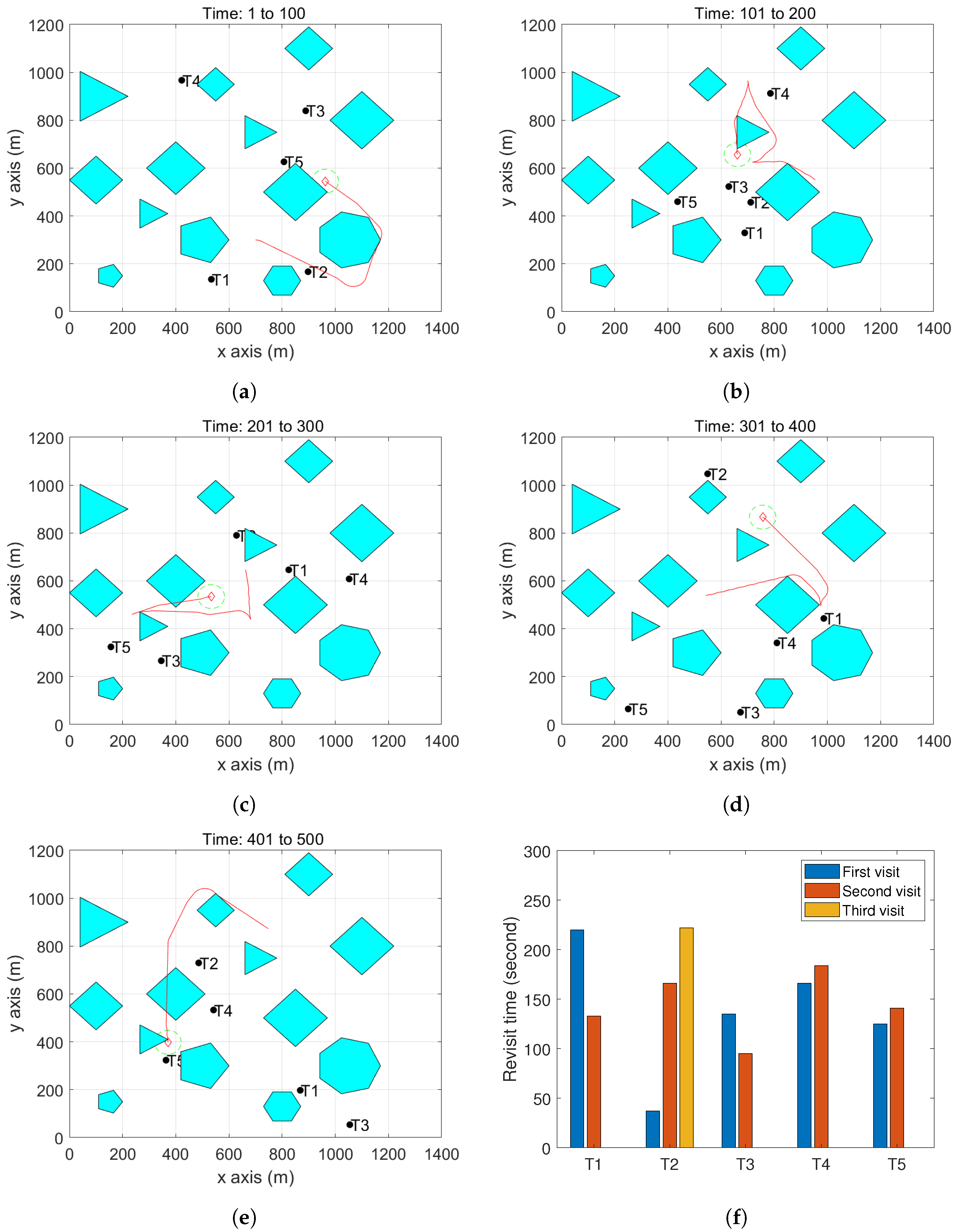
We first consider using one UAV to survey the targets. The used parameters are listed, as follows: $V^{max}=10$ m/s, ${\Omega }^{max}=0.5$ rad/s, $z=65$ m, $R=50$ m, $T=500$ s and $\sigma =0$. It is worth pointing out that the parameters of $V^{max}$ and ${\Omega }^{max}$ depend on the maneuverability of the UAV in use. Our method is not restricted to these parameters. The function $\gamma \left(t\right)$ is set to be increasing linearly with time. As will be seen in the below results, because the UAV flight height is taller than some buildings and lower than the others, a UAV needs to avoid the taller buildings but can fly above the lower buildings. To make results more understandable, we assume that during the 500 s, the incidence angle does not change. The fixed value can response to the average value during the 500 s. Subsequently, we can pre-compute the shadow range. Similar to ${\mathcal{X}}_{building}$, the shadow region is not allowed for the UAV to enter. Given an initial state, the trajectory of the UAV is obtained by applying Algorithm 2. In particular, the randomized Algorithm 1 is used to generate UAV trajectories to intercept the five targets. In our simulation, for the case with five targets, Algorithm 1 (runs on a normal computer with an Intel(R) Core(TM) i7-8565U CPU and 8.00 G RAM) takes less than 1 s to return five random trajectories. Although the onboard processor may not be as powerful as a normal computer, the algorithm can be coded in the more efficient language C. Moreover, even if the practical computation time may be longer than the simulation environment, in practice, the UAV can start to compute the random trajectories before it intercepts the intended target. Experimental verification of the proposed methods is left as our future work.

To make the trajectories visible, we demonstrate the 2D views in Figure 8 for each period of 100 s. We also record the movements of the UAV and the targets in some videos, and links for both 2D and 3D views are available at the caption of Figure 8. From Figure 8f, we can see that the five targets are visited twice or three times in the operation period, and the maximum revisit time is about 220 s. For the same targets movements, we increase the maximum of the UAV linear speed to $V^{max}=15$ m/s, and the UAV’s trajectory is shown in Figure 9. From Figure 9f, we can see that target 1 was visited three times and all the other targets are visited four times in the operation. The maximum revisit time is reduced from 220 s to 180 s.

Finally, we add one more UAV to survey the same targets. Here, $V^{max}=10$ m/s, and all of the other parameters remain the same as above. We show the trajectories of the two UAVs in Figure 10. From Figure 10f we can see that compared to the results by one UAV, the maximum revisit time is reduced from 220 s to 150 s. The maximum angular speeds, i.e., ${\Omega }^{max}$, has little impact on the maximum revisit time, since it only influences the UAV trajectory when the UAV makes a turn.

6. Conclusions

We considered using UAVs to conduct periodical surveillance of moving targets. We formulated an optimization problem in order to minimize the target revisit time. We proposed autonomous navigation algorithms for different cases. Because these algorithms are based on RRT, they inherit the advantage of computational efficiency, and they are promising to be applied in real-time. The simulation results showed their effectiveness.

One limitation of the current work lies in the assumption that the targets’ trajectories are known. When these trajectories are unavailable, the accuracy of the target position predictions may significantly decrease. Consequently, the UAVs may lose some targets. One future research work is to extend the algorithms by including the searching operation. Another direction is to conduct experiments, since this is the most effective way to practically verify the computational efficiency of the proposed method. To this end, some ground mobile robots can play the role of targets and a small number of UAVs can be tested in order to conduct the surveillance mission in a laboratory environment.