Day-Ahead and Intra-Day Collaborative Optimized Operation among Multiple Energy Stations

Abstract

An integrated energy system (IES) shows great potential in reducing the terminal energy supply cost and improving energy efficiency, but the operation scheduling of an IES, especially integrated with inter-connected multiple energy stations, is rather complex since it is affected by various factors. Toward a comprehensive operation scheduling of multiple energy stations, in this paper, a day-ahead and intra-day collaborative operation model is proposed. The targeted IES consists of electricity, gas, and thermal systems. First, the energy flow and equipment composition of the IES are analyzed, and a detailed operation model of combined equipment and networks is established. Then, with the objective of minimizing the total expected operation cost, a robust optimization of day-ahead and intra-day scheduling for energy stations is constructed subject to equipment operation constraints, network constraints, and so on. The day-ahead operation provides start-up and shut-down scheduling of units, and in the operating day, the intra-day rolling operation optimizes the power output of equipment and demand response with newly evolved forecasting information. The photovoltaic (PV) uncertainty and electric load demand response are also incorporated into the optimization model. Eventually, with the piecewise linearization method, the formulated optimization model is converted to a mixed-integer linear programming model, which can be solved using off-the-shelf solvers. A case study on an IES with five energy stations verifies the effectiveness of the proposed day-ahead and intra-day collaborative robust operation strategy.

1. Introduction

At present, the global energy market is extremely unstable, and energy has become an important factor affecting the economic development of many countries. As a new generation of energy supply systems, the integrated energy system (IES) can make full use of the complementary characteristics of gas, cold, heat, and electric energy, while reducing the cost of regional energy supply and improving the stability of terminal energy supply. However, as an IES integrates the production, conversion, and use of gas, cold, heat, and electric energy, many uncontrollable and uncertain factors are involved. This also makes the scheduling operation of an IES greatly challenging [1].

In [2,3,4], considering the economic and environmental factors of an IES, the multi-objective optimization operation model was established to dispatch the multi-energy equipment in the system. Ju et al. [5] proposed a micro-grid energy management method including energy storage equipment, which can reduce system operation cost and enhance system reliability. Pan et al. [6] studied the optimal operation method of electricity–heat supply of building an IES considering heat storage. For an IES including wind power, photovoltaic (PV) power, and other renewable energy generation devices, there are studies on improving the new energy consumption through cold and thermal energy storage so as to solve the uncertainty problem of renewable energy output. Tan et al. [7] studied the method of improving the operation efficiency of a micro-grid based on advanced energy storage technology. In [8], a multi-source coordinated energy storage system consisting of electricity, heat, and hydrogen was established, and coordinated optimization was carried out through a multi-energy storage and conversion model so as to improve the regulation flexibility and economy of power grids. Zeng et al. [9] proposed a stability evaluation method including electro-pneumatic transformation and a nature gas storage system. Chen et al. and Fan et al. [10,11] established a hybrid energy storage system model and proposed a coordinated operation strategy of electric and thermal energy storage. With important coupling of the power grid and heat supply network, Chen et al. [12] established a model of combined heat and power (CHP) units and analyzed the influence of a heat storage tank on the economic operation of an IES. On the basis of the operation characteristics of the heat supply network, Li et al. [13] considered the thermoelectric hybrid scheduling model of various types of equipment, such as heat storage and wind power heating equipment. The wind power consumption ratio was effectively increased through the coordinated spatial and temporal scheduling of multiple energy sources.

The integrated energy system faces uncertainties on the energy supply and demand sides [14,15,16,17]. For the supply side, the most common uncertainty comes from the output uncertainty of renewable energy [18,19]. To reduce the impact of renewable energy output uncertainty on system operation scheduling, uncertainty optimization methods or prediction time shortening can be used to improve the prediction accuracy. Uncertainty optimization methods are divided into stochastic programming and robust optimization. Wang et al. [20] simulated the randomness of wind power output and power load demand and established an optimization model with the objective of minimizing the system operation cost, maximizing the power supply reliability and comprehensive benefits, while optimizing the output of each unit by using a genetic algorithm. Pazouki et al. [21] used the scenario analysis method to describe the uncertainty of renewable energy output and load and generated a large number of wind power and load forecast scenarios. The deterministic optimization for multiple scenarios was also carried out. Moreira et al. and Baringo and Baringo [22,23] studied the robust optimal operation method of an IES. Wu et al. [24] proposed a control strategy to improve the security and economy of an IES through multi-time scale scheduling. Rong et al. [25] proposed a coordinated control strategy of adding heat storage and electric boiler in the electricity–heat system, and through the two-stage rolling scheduling mode, the additional heat sources and unit output are reasonably arranged to effectively alleviate the serious phenomenon of wind abandonment under a high penetration rate of wind power.

During the operation of an IES, it is necessary to consider the constraints of gas, electric, cold, and heat transfer networks [26]. The power networks in an IES are generally low-voltage or medium-voltage distribution networks. At present, the research on distribution network modeling and solutions is relatively mature. Forward-backward generation, genetic algorithms, and many other solving algorithms can be used as solutions. In the aspect of modeling and solving the heat supply network, Li et al. and Shao et al. [27,28] considered the heat storage capacity of a hot-water pipeline in unit commitment and economic dispatch and adopted the temperature regulation range of a heat supply network node as the heat storage constraint. Wu et al. [29] linearized the nonlinear model in an IES and studied the optimal power flow algorithm of the IES based on mixed integer linear programming (MILP). In [30], the nighttime heat load was translated based on analyses of the thermal dynamic characteristics of the heat supply network and heating region. These studies showed that considering the thermodynamic characteristics of a heat supply network and buildings in the model is helpful to smooth the fluctuation of wind power and effectively reduce the proportion of wind power curtailment at night. Lu et al. [31] studied the modeling and optimal operation method of an IES considering thermal inertia. Different from the transfer of electric energy, the transfer of heat energy in the heat supply network can be realized through quality and quantity control. Quality control refers to adjusting the temperature of the supply and return of medium water to regulate the heat transfer power, and quantity control refers to adjusting the flow of medium water. This paper adopts the method of quality control [26].

An IES contains various types of energy load and has great potential of load demand response. The demand response potential can be released through the multi-energy complementarity of load, and thus the operation cost can be reduced. In [32], to improve the utilization rate of wind power, considering the demand side response of a micro-grid, an optimal scheduling model of a micro-grid with multi-source energy storage based on the price incentive demand response was established. Considering the uncertainty of the micro-grid, Geramifar et al. [33] coordinated multi-energy storage and load side demand response resources and proposed a joint optimization method. Nguyen and Le [34] set the indoor temperature change in buildings with comprehensive energy within a certain range and took electric vehicles as adjustable loads to participate in dispatching. Tabar et al. [35] studied the renewable energy in an IES as a demand response participant to promote the complementary consumption of renewable energy and improve the operation economy of the system.

To sum up, an IES has great potential in improving the regional energy supply economy and energy supply stability, and several optimization methods have been developed to deal with uncertainty factors in the IES. However, at present, the research on IESs mostly focuses on a certain factor for in-depth analysis. For example, some research ignores the energy network among multiple energy stations, where only equipment constraints are incorporated. Some others focus on the bi-direct conversion only between electrical power and another energy form, such as heat, cold, or gas. There is no overall consideration of an IES with full coupling among all types of energy forms.

Focusing on multiple energy stations belonging to one operator, this paper proposes a day-ahead and intra-day collaborative robust optimization operation method, considering the load demand response of electrical power and multi-energy storage. Full coupling among electricity, heat, cold, and gas with each energy station is captured. A case study demonstrates that the proposed method can reduce the operation cost of an IES by optimizing the equipment operation state.

The main contributions of the work are as follows:

• Combined with typical IES equipment models, the energy constraints of the pipe network, including electric, gas, heating, and cooling networks, are integrated toward a more detailed and comprehensive model for IES operation.
• Considering the uncertainty of the PV output, a day-ahead and intra-day collaborative robust optimization model of multiple energy stations is constructed, where the influence of electrical load participating in the demand response is also incorporated.
• The piecewise linearization method is used since the equipment and network model of an IES contains a large number of nonlinear terms. The whole optimization model is then converted to a mixed-integer linear programming model. Compared to other existing methods, a unified solution method for the optimal operation of equipment and the network in an IES is proposed.

The rest of this paper is structured as follows. In Section 2, modeling of the equipment and network of an IES is presented. In Section 3, the day-ahead and intra-day collaborative robust optimal operation model is formulated. In Section 4, a case study on an IES with multiple energy stations is presented, and Section 5 draws conclusions.

2. Integrated Energy System Modeling

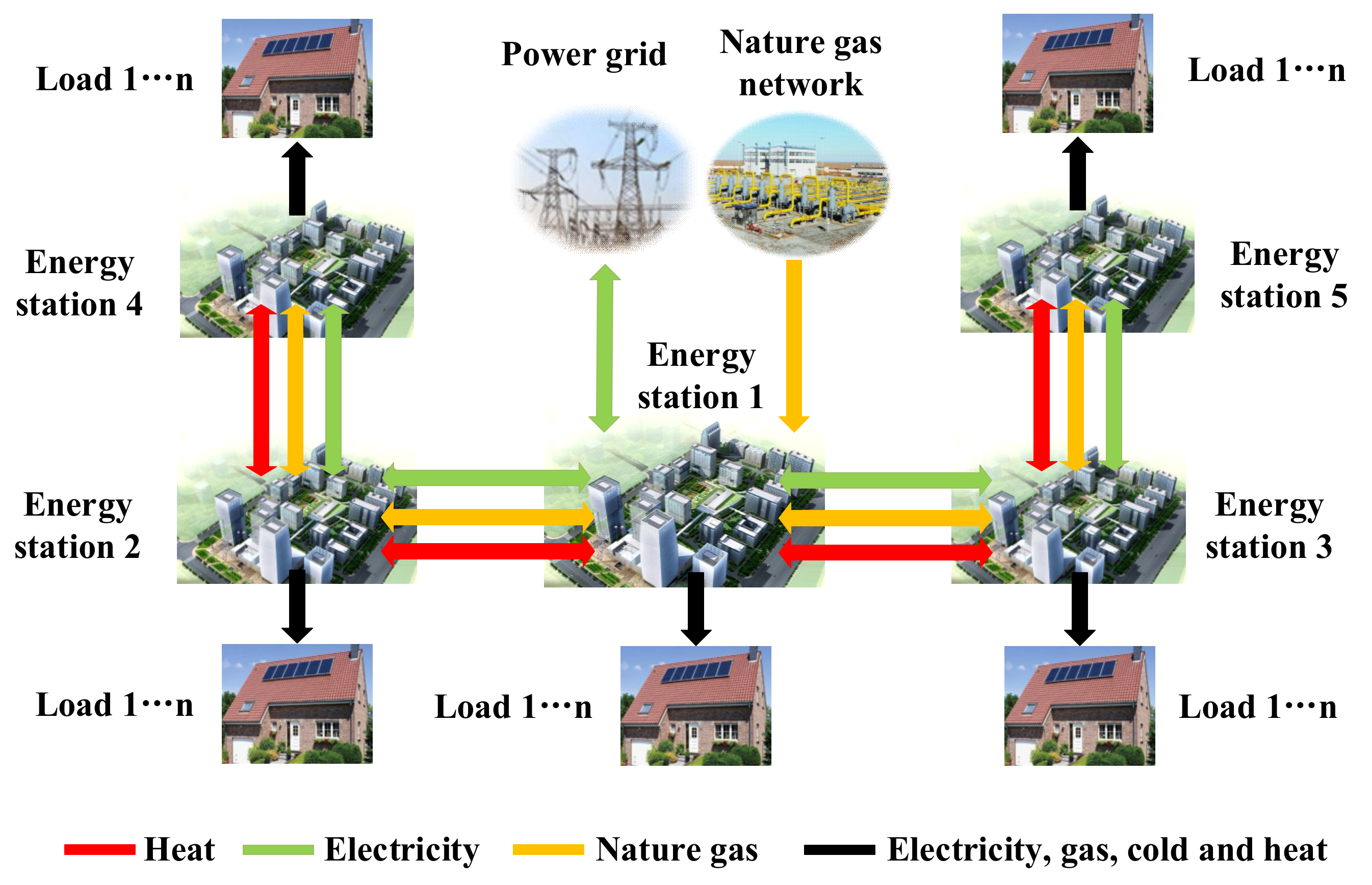
2.1. An Overview of Integrated Energy Systems

An integrated energy system is a terminal energy supply system, which is generally used in areas with concentrated cold, heat, electric, and gas loads. According to the energy supply scale, IESs can be divided into small, medium, and large IESs. For the medium-size or larger regional IESs, there may be multiple energy centers (energy stations). Each energy station can be connected through the distribution network, hot-water pipeline network, and urban gas pipeline, and multiple energy stations can work together to realize safe, stable, and efficient energy supply within the region. The energy flow network of the regional IES studied in this paper is shown in Figure 1. The topological structure of internal equipment in energy station 1 is shown in Figure 2. The main equipment in the energy station includes a combined cool heat and power (CCHP) unit, a waste heat boiler (WHB), a lithium bromide refrigeration (LR) unit, a gas boiler (GB), a heat pump (HP), an electric refrigerator (ER), electric energy storage (ES), heat energy storage (HS), cold energy storage (CS), PV generation equipment, and so on.

In the IES shown in Figure 1, each energy station is responsible for the energy supply of multiple energy loads within the service scope of the station. The energy stations are also connected through the power grid, the heat supply network, and gas pipelines. However, due to the energy loss in the transfer process, each energy station will give priority to meet the load within its supply scope to reduce the losses.

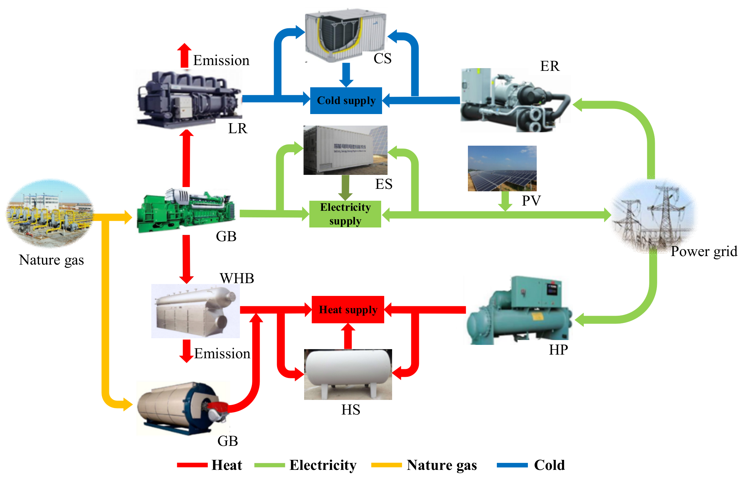
2.2. Equipment Modeling of an Integrated Energy System

2.2.1. CCHP Unit of the Gas Turbine

As the most important multi-energy coupling equipment in a regional comprehensive energy system, a gas turbine (GT) unit can efficiently convert natural gas into electric energy, heat energy, and cold energy. A conversion model of different kinds of energy in CCHP can be constructed. The energy conversion diagram of CCHP is as shown in Figure 3.

$$F_{\mathrm{CCHP},\mathrm{g}}^{}\left(t\right)=u_{\mathrm{CCHP}}\left(t\right)\times \frac{P_{\mathrm{CCHP},\mathrm{e}}^{}\left(t\right)}{{\eta }_{\mathrm{CCHP},\mathrm{e}}^{}\left(t\right)\times LHV}$$

(1)

$${\eta }_{\mathrm{CCHP},\mathrm{e}}^{}\left(t\right)=a_{\mathrm{CCHP}}\times {\left(\frac{P_{\mathrm{CCHP},\mathrm{e}}^{}\left(t\right)}{P_{\mathrm{CCHP},\mathrm{e}}^{\mathrm{N}}}\right)}^3+b_{\mathrm{CCHP}}\times {\left(\frac{P_{\mathrm{CCHP},\mathrm{e}}^{}\left(t\right)}{P_{\mathrm{CCHP},\mathrm{e}}^{\mathrm{N}}}\right)}^2+c_{\mathrm{CCHP}}\times \left(\frac{P_{\mathrm{CCHP},\mathrm{e}}^{}\left(t\right)}{P_{\mathrm{CCHP},\mathrm{e}}^{\mathrm{N}}}\right)+d_{\mathrm{CCHP}}$$

(2)

$$P_{\mathrm{WHB},\mathrm{h}}^{}\left(t\right)=\frac{u_{\mathrm{CCHP}}\left(t\right)\times \left(1-{\eta }_{\mathrm{CCHP},\mathrm{e}}^{}\left(t\right)-{\eta }_{\mathrm{CCHP}}^{\mathrm{loss}}\right)\times P_{\mathrm{CCHP},\mathrm{e}}^{}\left(t\right)}{{\eta }_{\mathrm{CCHP},\mathrm{e}}^{}\left(t\right)}$$

(3)

$$P_{\mathrm{CCHP},\mathrm{c}}^{}\left(t\right)=u_{\mathrm{CCHP}}\left(t\right)\times P_{\mathrm{LR},\mathrm{h}}^{}\left(t\right)\times CO{P}_{\mathrm{LR}}$$

(4)

$$P_{\mathrm{CCHP},\mathrm{h}}^{}\left(t\right)=P_{\mathrm{WHB},\mathrm{h}}^{}\left(t\right)-P_{\mathrm{LR},\mathrm{h}}^{}\left(t\right)$$

(5)

where $F_{\mathrm{CCHP},\mathrm{g}}^{}\left(t\right)$ is the natural gas consumption of the CCHP unit in time period t, m³/h; $u_{\mathrm{CCHP}}\left(t\right)$ refers to the on and off status of the CCHP unit in time period t; 1 indicates the unit is on and 0 indicates off; $P_{\mathrm{CCHP},\mathrm{e}}^{}\left(t\right)$ is the electrical output power of the CCHP unit in time period t, kW; $P_{\mathrm{CCHP},\mathrm{e}}^{\mathrm{N}}$ is the rated electric power of the CCHP unit; LHV is the low calorific value of natural gas, taking 9.7 kWh/m³; $a_{\mathrm{CCHP}}$, $b_{\mathrm{CCHP}}$, $c_{\mathrm{CCHP}}$, and $d_{\mathrm{CCHP}}$ are the generation efficiency function coefficients of the CCHP unit; ${\eta }_{\mathrm{CCHP},\mathrm{e}}^{}\left(t\right)$ is the generation efficiency of the CCHP unit in time period t; ${\eta }_{\mathrm{CCHP}}^{\mathrm{loss}}$ is the thermal energy self-dissipation rate of the CCHP unit; $P_{\mathrm{WHB},\mathrm{h}}^{}\left(t\right)$ is the output thermal power of the waste heat recovery boiler of the CCHP unit in time period t, kW; $P_{\mathrm{CCHP},\mathrm{h}}^{}\left(t\right)$ is the output heat power of the CCHP unit in time period t, kW; $P_{\mathrm{LR},\mathrm{h}}^{}\left(t\right)$ is the thermal power absorbed by LR from the GT, kW; $CO{P}_{\mathrm{LR}}$ refers to the hot and cold conversion efficiency of LR; and $P_{\mathrm{CCHP},\mathrm{c}}^{}\left(t\right)$ refers to the output cooling power of the CCHP unit, kW.

2.2.2. Gas Boiler

With a gas boiler, natural gas converts its chemical energy into thermal energy. Thermal energy is transferred to users through water.

$$F_{\mathrm{GB},\mathrm{g}}^{}\left(t\right)=u_{\mathrm{GB}}\left(t\right)\times P_{\mathrm{GB},\mathrm{h}}^{}\left(t\right)/\left({\eta }_{\mathrm{GB}}\times LHV\right)$$

(6)

where $F_{\mathrm{GB},\mathrm{g}}^{}\left(t\right)$ is the natural gas consumption of the GB in time period t, m³/h; $u_{\mathrm{GB}}\left(t\right)$ refers to the start-up and shut-down status of the GB in time period t; 1 indicates the unit is on and 0 indicates off; $P_{\mathrm{GB},\mathrm{h}}^{}\left(t\right)$ is the output thermal power of the GB in time period t, kW; and ${\eta }_{\mathrm{GB}}^{}$ is the heat production efficiency of the GB.

2.2.3. Electric Refrigeration

ER does not directly produce cold energy but releases the heat energy in the system to the outside. Therefore, the refrigeration capacity of electric refrigeration is related to its refrigeration coefficient.

$$P_{\mathrm{ER},\mathrm{c}}^{}\left(t\right)=P_{\mathrm{ER},\mathrm{e}}^{}\left(t\right)\times CO{P}_{\mathrm{ER}}$$

(7)

where $P_{\mathrm{ER},\mathrm{e}}^{}\left(t\right)$ is the electric power consumed by the ER unit in time period t, kW; $P_{\mathrm{ER},\mathrm{c}}^{}\left(t\right)$ is the cooling energy power produced in time period t, kW; and $CO{P}_{\mathrm{ER}}$ is the refrigeration coefficient.

2.2.4. Heat Pump

The working principle of an HP is to collect the low-grade heating energy in the environment by consuming a small amount of electricity for heating objects.

$$P_{\mathrm{HP},\mathrm{h}}^{}\left(t\right)=P_{\mathrm{HP},\mathrm{e}}^{}\left(t\right)\times CO{P}_{\mathrm{HP}}$$

(8)

where $P_{\mathrm{HP},\mathrm{e}}^{}\left(t\right)$ is the electric power consumed by the HP in time period t, kW; $P_{\mathrm{HP},\mathrm{h}}^{}\left(t\right)$ is the thermal power output by the HP in time period t, kW; and $CO{P}_{\mathrm{HP}}$ is the heating coefficient of the HP.

2.2.5. Multi-Energy Storage

The configuration of cooling, thermal, and electric energy storage equipment in an IES can make full use of the physical complementary characteristics of cooling, thermal, and electric energy. Especially with CCHP units, efficient energy utilization can be achieved.

$$\left\{\begin{array}{l}{E}_{\mathrm{ES}}(t)=E_{\mathrm{ES}}(t-1)\times (1-{\delta }_{\mathrm{ES}}\times \Delta t)+\left(P_{\mathrm{ES}}^{\mathrm{cha}}(t)\times {\eta }_{\mathrm{ES}}^{\mathrm{cha}}-\frac{P_{\mathrm{ES}}^{\mathrm{dis}}(t)}{{\eta }_{\mathrm{ES}}^{\mathrm{dis}}}\right)\times \Delta t\\ E_{\mathrm{HS}}(t)=E_{\mathrm{HS}}(t-1)\times (1-{\delta }_{\mathrm{HS}}\times \Delta t)+\left(P_{\mathrm{HS}}^{\mathrm{cha}}(t)\times {\eta }_{\mathrm{HS}}^{\mathrm{cha}}-\frac{P_{\mathrm{HS}}^{\mathrm{dis}}(t)}{{\eta }_{\mathrm{HS}}^{\mathrm{dis}}}\right)\times \Delta t\\ E_{\mathrm{CS}}(t)=E_{\mathrm{CS}}(t-1)\times (1-{\delta }_{\mathrm{CS}}\times \Delta t)+\left(P_{\mathrm{CS}}^{\mathrm{cha}}(t)\times {\eta }_{\mathrm{CS}}^{\mathrm{cha}}-\frac{P_{\mathrm{CS}}^{\mathrm{dis}}(t)}{{\eta }_{\mathrm{CS}}^{\mathrm{dis}}}\right)\times \Delta t\end{array}\right.$$

(9)

where $E_{\mathrm{ES}}(t)$, $E_{\mathrm{HS}}(t)$, and $E_{\mathrm{CS}}(t)$ are the electric, heating, and cooling energy storage in time period t, respectively, kWh; $E_{\mathrm{ES}}(t-1)$, $E_{\mathrm{HS}}(t-1)$, and $E_{\mathrm{CS}}(t-1)$ are the electrical, heating, and cooling energy storage in time period t – 1, respectively, kWh; ${\delta }_{\mathrm{ES}}$, ${\delta }_{\mathrm{HS}}$, and ${\delta }_{\mathrm{CS}}$ are the self-energy consumption rates of electric, heating, and cooling energy storage, respectively, h⁻¹; $\Delta t$ is the unit-optimized operation interval, h; $P_{\mathrm{ES}}^{\mathrm{cha}}(t)$ and $P_{\mathrm{ES}}^{\mathrm{dis}}(t)$ are the charging and discharging power of electric energy storage, respectively, in time period t, kW; $P_{\mathrm{HS}}^{\mathrm{cha}}(t)$ and $P_{\mathrm{HS}}^{\mathrm{dis}}(t)$ are the charging and discharging power of heat energy storage, respectively, in time period t, kW; $P_{\mathrm{CS}}^{\mathrm{cha}}(t)$ and $P_{\mathrm{CS}}^{\mathrm{dis}}(t)$ are the charging and discharging power of cold energy storage, respectively, in time period t, kW; ${\eta }_{\mathrm{ES}}^{\mathrm{cha}}$ and ${\eta }_{\mathrm{ES}}^{\mathrm{dis}}$ are the charging and discharging efficiency of electric energy storage, respectively; ${\eta }_{\mathrm{HS}}^{\mathrm{cha}}$ and ${\eta }_{\mathrm{HS}}^{\mathrm{dis}}$ are the charging and discharging efficiency of heat energy storage, respectively, in time period t; and ${\eta }_{\mathrm{CS}}^{\mathrm{cha}}$ and ${\eta }_{\mathrm{CS}}^{\mathrm{dis}}$ are the charging and discharging efficiency, respectively, of the ice storage tank.

2.3. Modeling of the Multi-Energy Network

An integrated energy system consists of several energy stations. Different energy stations are responsible for meeting the multi-energy load demand of the region. The energy stations are connected through natural gas pipelines, power networks, and hot-water pipelines to complete the transfer of natural gas, electric energy, and heat energy between stations in the IES. For the rest of this paper, we assume that the inner network constraints within each energy station can be ignored, and we only focus on networks connecting energy stations.

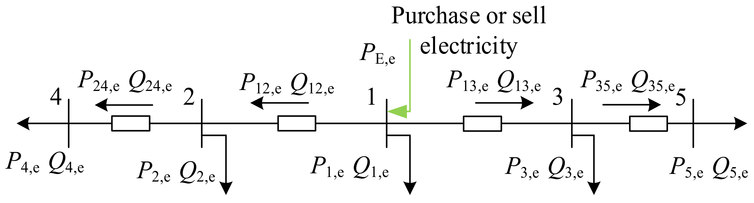
2.3.1. Electrical Power Network

The electrical distribution network with energy stations is constructed, which is in radial topology, as shown in Figure 4; each node represents one energy station. The electrical losses on network sections are ignored, since energy stations are closely located.

The active power balance equation among the energy stations is as follows:

$$\left\{\begin{array}{l}{P}_{1,\mathrm{e}}^{}=-P_{12,\mathrm{e}}^{}-P_{13,\mathrm{e}}^{}+P_{E,\mathrm{e}}^{}\\ P_{2,\mathrm{e}}^{}=P_{12,\mathrm{e}}^{}-P_{24,\mathrm{e}}^{}\\ P_{3,\mathrm{e}}^{}=P_{13,\mathrm{e}}^{}-P_{35,\mathrm{e}}^{}\\ P_{4,\mathrm{e}}^{}=P_{24,\mathrm{e}}^{}\\ P_{5,\mathrm{e}}^{}=P_{35,\mathrm{e}}^{}\end{array}\right.$$

(10)

The reactive power balance equation is similar to Equation (10). They can be summarized as

$$P_{i,\mathrm{e}}^{}\left(t\right)=-{\displaystyle \sum _{j\in \mathsf{\Omega }\left(i\right)}{P}_{ij,\mathrm{e}}^{}\left(t\right)}+P_{E,\mathrm{e}}^{}\left(t\right)$$

(11)

where $\mathsf{\Omega }\left(i\right)$ represents the energy stations that have connection to energy station i, $P_{ij,\mathrm{e}}^{}\left(t\right)$ is the active power transmitted by the power network from energy station i to j, $P_{i,\mathrm{e}}^{}\left(t\right)$ is the active power output of energy station i, $Q_{ij,\mathrm{e}}^{}\left(t\right)$ is the reactive power transmitted by the power network from energy station i to j, $Q_{i,\mathrm{e}}^{}\left(t\right)$ is the reactive power output of energy station i, and $P_{E,\mathrm{e}}^{}\left(t\right)$ is the electric power transmitted from the power network to the IES. The actual flow direction of active and reactive power is distinguished with positive and negative values of $P_{ij,\mathrm{e}}^{}\left(t\right)$ and $Q_{ij,\mathrm{e}}^{}\left(t\right)$.

The relationship between the node voltage of energy stations i and j and the power transferred between them is [36]:

$$U_i^2\left(t\right)-U_j^2\left(t\right)=2\left(r_{ij}^{}{P}_{ij,\mathrm{e}}^{}\left(t\right)+x_{ij}^{}{Q}_{ij,\mathrm{e}}^{}\left(t\right)\right)$$

(12)

where $U_i^2\left(t\right)$ and $U_j^2\left(t\right)$ represent the square of voltage value of energy stations i and j at time period t, respectively, and $r_{ij}^{}$ and $x_{ij}^{}$ represent the resistance and reactance values of power lines between energy stations i and j, respectively.

Except for the above lossless power flow equations, other operational constraints of an electrical distribution network are presented in Section 3.2.2 and Section 3.2.3, including node power injection in Equation (46), node voltage limits in Equation (49), and network line capacity constraints in Equation (50).

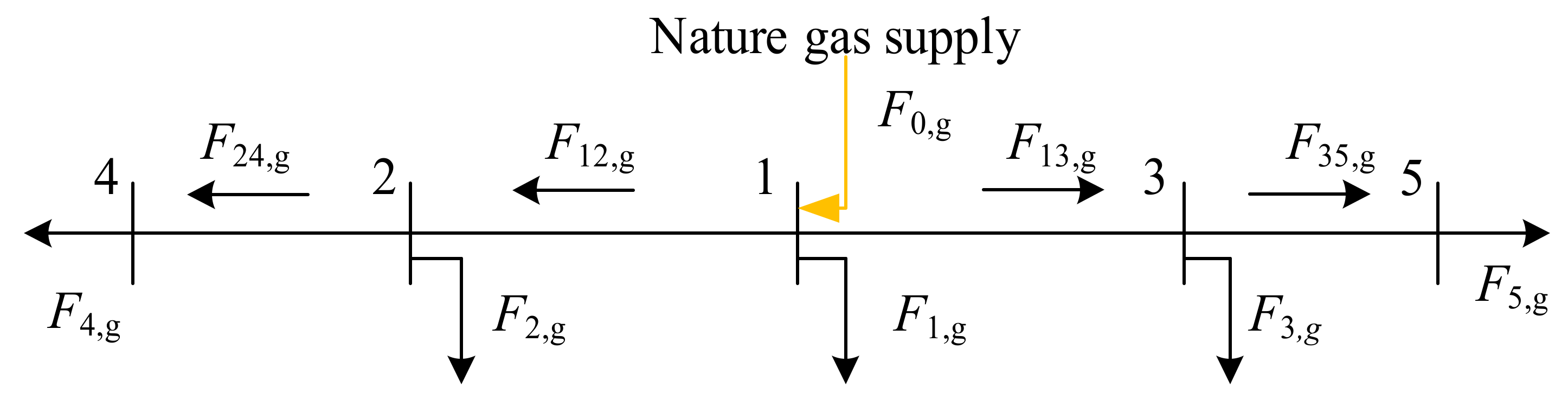
2.3.2. Natural Gas Network

The natural gas network topology of energy stations is shown in Figure 5. In Figure 5, the actual direction of gas flow, $F_{ij,\mathrm{g}}$, is distinguished with its positive and negative values.

Ignoring the change in pipeline height and the change in temperature at different positions of the pipeline, and ignoring the time dynamic process, the natural gas pipeline transfer model can be expressed as follows [37]:

$$F_{ij}\left(t\right)\cdot \left|F_{ij}\left(t\right)\right|=C_{ij}^2\left({\tau }_i^2\left(t\right)-{\tau }_j^2\left(t\right)\right)\forall i,j,t$$

(13)

where $F_{ij}\left(t\right)$ is the natural gas flow from energy station i to j, $C_{ij}^{}$ is the friction coefficient of natural gas pipeline ij, and ${\tau }_i^{}\left(t\right)$ is the natural gas pressure at energy station i. The allowable upper and lower limits for node gas pressure and the line capacity limit are presented in Equations (51) and (52) in Section 3.2.3.

During the operation process, natural gas pipelines between multi-energy stations need to satisfy not only pipeline pressure constraints but also node flow balance constraints, as shown in Equation (14).

$$F_{i,g}^{}\left(t\right)=-{\displaystyle {\sum }_{j\in \mathsf{\Omega }\left(i\right)}{F}_{ij,g}^{}\left(t\right)}+F_{0,g}^{}\left(t\right)$$

(14)

where $F_{i,g}^{}$ is the gas consumption of node i, $F_{ij,g}^{}$ is the natural gas flow of pipeline ij from i to j, and $F_{0,g}^{}$ is the gas provided by the city’s natural gas pipeline to a certain energy station. Since only energy station 1 is directly connected to the city’s natural gas pipeline, except for energy station 1, $F_{0,g}^{}$ of other energy stations should be 0. The expression of node gas consumption is presented in Equation (48) in Section 3.2.2.

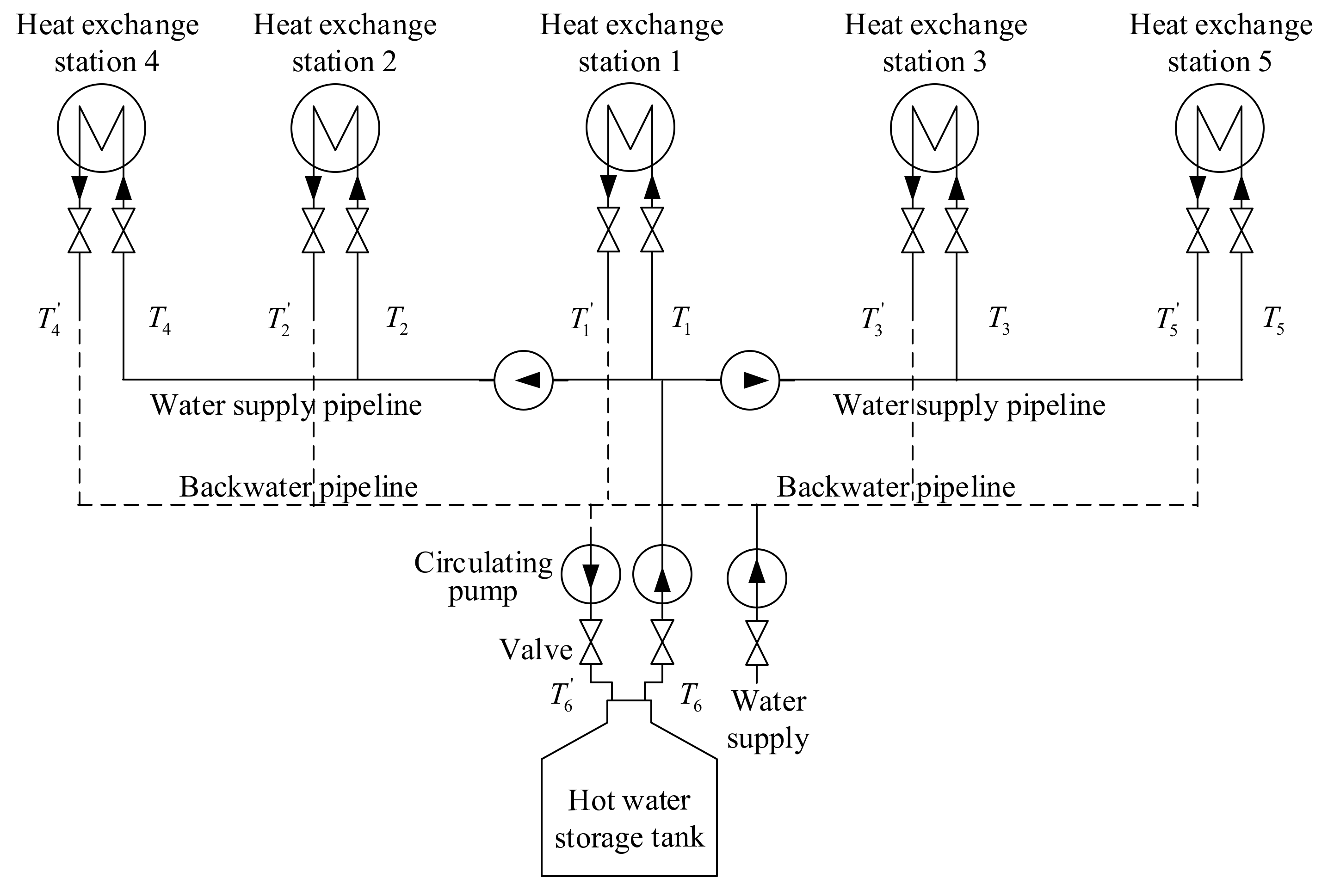
2.3.3. Thermal Network

Heat energy needs to be transmitted by a transfer medium, generally water. Only the primary heat supply network through which the heat transfers between energy stations is considered, while the secondary pipe network through which energy stations transfer heat energy to users is omitted. The heat transfer model is divided into a thermodynamic model and a hydraulic model. The pipe network diagram of a heating supply system is shown in Figure 6.

Thermodynamic Equations

The thermodynamic equations of hot-water pipelines are as follows:

$$P_k^h\left(t\right)=C_{\mathrm{w}}\cdot M_k\left(t\right)\cdot \left(T_k^{}\left(t\right)-T_k^{\prime }\left(t\right)\right)$$

(15)

$$T_j^{}\left(t\right)=T_i^{}\left(t\right){\varphi }_{ij}\left(t\right)$$

(16)

$$\left({\displaystyle \sum _{j\in {\mathsf{\Omega }}^{+}(i)}^{}{M}_{ij}\left(t\right)}\right)T_{ij}\left(t\right)={\displaystyle \sum _{j\in {\mathsf{\Omega }}^{-}(i)}^{}\left(M_{ji}\left(t\right)T_{ji}\left(t\right)\right)},\forall i$$

(17)

where $P_k^h\left(t\right)$ is the output heat power of energy station k; $C_{\mathrm{w}}$ is the specific heat capacity of medium water; $M_k$ is the hot-water flow of the heat exchanger at energy station k; $T_k^{}\left(t\right)$ and $T_k\prime \left(t\right)$ are the supply and return water temperatures at energy station k, respectively,; ${\varphi }_{ij}\left(t\right)$ is the temperature drop coefficient of pipeline ij; the environment temperature $T_a$ is 35 °C in summer, 20 °C in spring and autumn, and 0 °C in winter; $L_{ij}$ is the length of pipeline ij; and $\lambda$ is the heat conduction coefficient.

$$\left\{\begin{array}{l}{T}_i^{}\left(t\right)=T_i^{\prime }\left(t\right)-T_a\\ T_j\left(t\right)=T_j^{\prime }\left(t\right)-T_a\\ \varphi \left(t\right)=e^{-\lambda L_{ij}/C_{\mathrm{w}}{M}_{ij}\left(t\right)}\end{array}\right.$$

(18)

The temperature constraint of the supply and return water of nodes is given in Equation (53) in Section 3.2.3.

Hydraulic Equations

The flow balance equation of the hydraulic network for node j is as follows:

$$\left\{\begin{array}{l}{A}_h\left(t\right)\cdot M_{ij}\left(t\right)=M_j\left(t\right)\\ B_h\left(t\right)\cdot M_{ij}^T\left(t\right)diag(K_{ij})\left|M_{ij}\left(t\right)\right|=0\end{array}\right.,i\in \mathsf{\Omega }(j),\forall j$$

(19)

where A_h(t) is the heat supply network correlation matrix, B_h(t) is the basic loop matrix; M_ij(t) is the pipeline flow vector, M_j(t) is the inflow flow vector of each node, $K_{ij}$ is the pipeline impedance coefficient, $i\in \mathsf{\Omega }\left(j\right)$ means that node i is directly connected to node j, and T is the total number of optimized time intervals in one day. The constraint of hot-water flow in pipelines is given in Equation (54) in Section 3.2.3.

With constant flow in hot-water pipelines and variable temperatures in the heat transfer mode, the thermal equations of hot-water pipelines are linear equations, and the heat transfer capacity of a hot-water pipe network is related to the hot-water flow.

3. Day-Ahead and Intra-Day Collaborative Robust Optimization Model for an IES

Based on the equipment and network model of an IES and considering the constraints of the equipment and network operation, a day-ahead and intra-day collaborative robust optimization model is constructed in this section. According to the prediction data, the day-ahead optimal operation scheme of the IES is obtained. On the basis of day-ahead optimal operation scheduling, considering the constraints of the units’ on/off status and equipment output adjustment, the intra-day rolling optimal operation strategy of the IES is constructed. The optimal scheduling scheme of the IES is obtained according to the rolling forecast data.

The optimization objective is to minimize the total operation cost of multi-energy stations based on the ultra-short-term forecasting data of cold, heat, and electricity loads and PV generation output, satisfying the operation constraints of the system and equipment. The optimized variables include the equipment output of the CCHP unit, the HP, the ER, and the GB and the electricity purchased from the grid. Through the day-head pre-dispatch and rolling intra-day operation, the most economical coordinated operation scheduling results of multiple energy stations in the IES can be obtained.

3.1. Objective Functions

3.1.1. Objective Function of Day-Ahead Optimized Operation of the IES

Considering the uncertainty of the PV output, the objective function of the day-ahead economic robust optimization of the IES is constructed. The objective is to minimize the total operation cost, including the fuel cost, electricity cost, start-up and shutdown cost, maintenance cost, and demand response income.

$$\underset{x\in X}{\min }\underset{w\in W}{\max }\left(C_F+C_E+C_S+C_M-C_R\right)$$

(20)

$$C_F={\displaystyle \sum _{t=1}^T{\displaystyle \sum _{k=1}^{{\mathrm{N}}_{\mathrm{S}}}\left(c_f\cdot F_{\mathrm{CCHP},\mathrm{g},k}^{}\left(t\right)\cdot \Delta t\right)}}+{\displaystyle \sum _{t=1}^T{\displaystyle \sum _{k=1}^{{\mathrm{N}}_{\mathrm{S}}}\left(c_f\cdot F_{\mathrm{GB},\mathrm{g},k}^{}\left(t\right)\cdot \Delta t\right)}}$$

(21)

$$C_{\mathrm{E}}={\displaystyle \sum _{t=1}^T\left(c_{\mathrm{b},\mathrm{e}}\left(t\right)\cdot P_{\mathrm{b},\mathrm{E},\mathrm{e}}^{}\left(t\right)-c_{\mathrm{s},\mathrm{e}}\left(t\right)\cdot P_{\mathrm{s},\mathrm{E},\mathrm{e}}^{}\left(t\right)\right)\cdot \Delta t}$$

(22)

$$C_{\mathrm{S}}={\displaystyle \sum _{t=1}^T{\displaystyle \sum _{k=1}^{{\mathrm{N}}_{\mathrm{S}}}{c}_{\mathrm{CCHP},k}\cdot \left|u_{\mathrm{CCHP},k}\left(t\right)-u_{\mathrm{CCHP},k}\left(t-1\right)\right|}}+{\displaystyle \sum _{t=1}^T{\displaystyle \sum _{k=1}^{{\mathrm{N}}_{\mathrm{S}}}{c}_{\mathrm{GB},k}\cdot \left|u_{\mathrm{GB},k}\left(t\right)-u_{\mathrm{GB},k}\left(t-1\right)\right|}}$$

(23)

$$C_{\mathrm{M}}={\displaystyle \sum _{t=1}^T{\displaystyle \sum _{k=1}^{{\mathrm{N}}_{\mathrm{S}}}\left(\begin{array}{l}{c}_{\mathrm{CCHP},k}^{\mathrm{m}}\cdot P_{\mathrm{CCHP},\mathrm{e},k}^{\mathrm{DA}}\left(t\right)+c_{\mathrm{GB},k}^{\mathrm{m}}\cdot P_{\mathrm{GB},\mathrm{h},k}^{\mathrm{DA}}\left(t\right)+\\ c_{\mathrm{PV},k}^{\mathrm{m}}\cdot P_{\mathrm{PV},\mathrm{e},k}^{\mathrm{DA}}\left(t\right)+c_{\mathrm{HP},k}^{\mathrm{m}}\cdot P_{\mathrm{GB},\mathrm{h},k}^{\mathrm{DA}}\left(t\right)+\\ c_{\mathrm{ER},k}^{\mathrm{m}}\cdot P_{\mathrm{GB},\mathrm{h},k}^{\mathrm{DA}}\left(t\right)+c_{\mathrm{ES},k}^{\mathrm{m}}\cdot (P_{\mathrm{ES},k}^{\mathrm{cha}}(t)+P_{\mathrm{ES},k}^{\mathrm{dis}}(t))+\\ c_{\mathrm{HS},k}^{\mathrm{m}}\cdot (P_{\mathrm{HS},k}^{\mathrm{cha}}(t)+P_{\mathrm{HS},k}^{\mathrm{dis}}(t))+c_{\mathrm{CS},k}^{\mathrm{m}}\cdot (P_{\mathrm{CS},k}^{\mathrm{cha}}(t)+P_{\mathrm{CS},k}^{\mathrm{dis}}(t))\end{array}\right)\cdot \Delta t}}$$

(24)

$$C_{\mathrm{R}}={\displaystyle \sum _{t=1}^T{\displaystyle \sum _{k=1}^{{\mathrm{N}}_{\mathrm{S}}}{c}_{\mathrm{R}}\cdot \left(P_{\mathrm{R},\mathrm{e},k}^{}\left(t\right)-P_{\mathrm{L},\mathrm{e},k}^{}\left(t\right)\right)}}$$

(25)

where x is the control variable, representing the output of the CCHP unit, the GB, the HP, the ER, and energy storage equipment; X is the control variable set, representing the output range of each equipment; $w$ is the uncertainty variable, representing the PV output, kW; $W$ is the uncertainty variable set, representing the error range of the PV output; $C_{\mathrm{F}}$, $C_{\mathrm{E}}$, $C_{\mathrm{S}}$, $C_{\mathrm{M}}$, and $C_{\mathrm{R}}$ are the fuel cost, electricity cost, start-up and shutdown cost, maintenance cost, and demand response income, respectively; $k$ represents the k-th energy station; $N_{\mathrm{S}}$ is the number of energy stations; $F_{\mathrm{CCHP},\mathrm{g},k}^{}\left(t\right)$ is the gas consumption of the CCHP unit in energy station s in time period t; $T$ is the total number of time periods in a single day; $c_f$ is the unit price of natural gas; $c_{\mathrm{b},}{}_{\mathrm{e}}\left(t\right)$ and $c_{\mathrm{s},}{}_{\mathrm{e}}\left(t\right)$ represent the purchase and sale price of electricity per kilowatt hour, respectively; $P_{\mathrm{b},\mathrm{E},}{}_{\mathrm{e}}\left(t\right)$ and $P_{\mathrm{s},\mathrm{E},}{}_{\mathrm{e}}\left(t\right)$ represent the purchase and sale electrical power, respectively; $c_{\mathrm{CCHP},k}$ and $c_{\mathrm{GB},k}$ represent for the start-up and shut-down cost of the CCHP unit and gas-fired boiler, respectively; $c_{\mathrm{CCHP},k}^{\mathrm{m}}$, $c_{\mathrm{GB},k}^{\mathrm{m}}$, $c_{\mathrm{PV},k}^{\mathrm{m}}$, $c_{\mathrm{HP},k}^{\mathrm{m}}$, $c_{\mathrm{ER},k}^{\mathrm{m}}$, $c_{\mathrm{ES},k}^{\mathrm{m}}$, $c_{\mathrm{HS},k}^{\mathrm{m}}$, and $c_{\mathrm{CS},k}^{\mathrm{m}}$ are the maintenance cost of the CCHP, GB, PV, HP, ER, ES, HS, and CS equipment of energy station k, respectively; $P_{\mathrm{CCHP},\mathrm{e},k}\left(t\right)$ is the electricity output of the CCHP unit of energy station k; $P_{\mathrm{GB},\mathrm{e},k}\left(t\right)$, $P_{\mathrm{PV},\mathrm{e},k}\left(t\right)$, and $P_{\mathrm{ER},\mathrm{e},k}\left(t\right)$ are the electricity consumption of the GB, PV, HP, and ER equipment of energy station k, respectively, in time period t; $P_{\mathrm{ES},k}^{\mathrm{cha}}(t)$, $P_{\mathrm{HS},k}^{\mathrm{cha}}(t)$ and $P_{\mathrm{CS},k}^{\mathrm{cha}}(t)$ are the charging power of electricity, heat, and cold energy storage of energy station k, respectively, in time period t; $P_{\mathrm{ES},k}^{\mathrm{dis}}(t)$, $P_{\mathrm{HS},k}^{\mathrm{dis}}(t)$, and $P_{\mathrm{CS},k}^{\mathrm{dis}}(t)$ are the discharging power of electricity, heat, and cold energy storage of energy station k, respectively, in t; $c_{\mathrm{R}}$ is the profit of electric load participating in demand response per kilowatt hour; $P_{\mathrm{L},\mathrm{e},k}^{}\left(t\right)$ is the forecasting electric load for time period t; and $P_{\mathrm{R},\mathrm{e},k}^{}\left(t\right)$ is the actual electric load after demand response in time period t.

3.1.2. Objective Function of Intra-Day Optimized Operation of an IES

Due to the errors in day-ahead forecast, there exist differences between the forecasted and the actually resolved PV power output and load values. The day-ahead pre-determined operation scheduling might not be feasible, and adjustment of unit power output might be needed. Therefore, during the operating day, rolling optimization is carried out on the basis of day-ahead scheduled equipment output and newly obtained forecast information. Compared with day-ahead optimization, rolling optimization does not consider adjustment of the equipment start-up and shut-down status. Therefore, the objective function does not consider the start-up and shut-down cost but includes the adjustment cost of equipment output. The correction amount constraints of day-ahead plan for each equipment and the state of charge constraints of energy storage are added. The optimization objective of the rolling operation is to minimize the operation cost in the periods from the decision-making point t₀ to the end of the operating day. The total number of operation time periods is T. The operation cost includes the natural gas purchase cost, electricity purchase cost, equipment maintenance cost, and equipment output adjustment cost. The objective function of day-ahead and intra-day collaborative optimization of an IES is as follows.

$$\underset{x\in X}{\min }\underset{w\in W}{\max }{\displaystyle \sum _{t=t_0}^T\left(C_{\mathrm{F}}\left(t\right)+C_{\mathrm{E}}\left(t\right)+C_{\mathrm{M}}\left(t\right)+C_{\mathrm{A}}\left(t\right)\right)}(25)$$

(26)

$$C_{\mathrm{F}}={\displaystyle \sum _{k=1}^{{\mathrm{N}}_{\mathrm{S}}}\left(c_f\cdot F_{\mathrm{CCHP},\mathrm{g},k}^{}\left(t\right)\cdot \Delta t\right)}+{\displaystyle \sum _{k=1}^{{\mathrm{N}}_{\mathrm{S}}}\left(c_f\cdot F_{\mathrm{GB},\mathrm{g},k}^{}\left(t\right)\cdot \Delta t\right)}(26)$$

(27)

$$C_{\mathrm{E}}=\left(c_{\mathrm{b},\mathrm{e}}\left(t\right)\cdot P_{\mathrm{b},\mathrm{E},\mathrm{e}}^{}\left(t\right)-c_{\mathrm{s},\mathrm{e}}\left(t\right)\cdot P_{\mathrm{s},\mathrm{E},\mathrm{e}}^{}\left(t\right)\right)\cdot \Delta t(27)$$

(28)

$$C_{\mathrm{M}}={\displaystyle \sum _{k=1}^{{\mathrm{N}}_{\mathrm{S}}}\left(\begin{array}{l}{c}_{\mathrm{CCHP},k}^{\mathrm{m}}\cdot P_{\mathrm{CCHP},\mathrm{e},k}\left(t\right)+c_{\mathrm{GB},k}^{\mathrm{m}}\cdot P_{\mathrm{GB},\mathrm{e},k}\left(t\right)+\\ c_{\mathrm{PV},k}^{\mathrm{m}}\cdot P_{\mathrm{PV},\mathrm{e},k}\left(t\right)+c_{\mathrm{HP},k}^{\mathrm{m}}\cdot P_{\mathrm{HP},\mathrm{e},k}\left(t\right)+\\ c_{\mathrm{ER},k}^{\mathrm{m}}\cdot P_{\mathrm{ER},\mathrm{e},k}\left(t\right)+c_{\mathrm{ES},k}^{\mathrm{m}}\cdot (P_{\mathrm{ES},k}^{\mathrm{cha}}(t)+P_{\mathrm{ES},k}^{\mathrm{dis}}(t))+\\ c_{\mathrm{HS},k}^{\mathrm{m}}\cdot (P_{\mathrm{HS},k}^{\mathrm{cha}}(t)+P_{\mathrm{HS},k}^{\mathrm{dis}}(t))+c_{\mathrm{CS},k}^{\mathrm{m}}\cdot (P_{\mathrm{CS},k}^{\mathrm{cha}}(t)+P_{\mathrm{CS},k}^{\mathrm{dis}}(t))\end{array}\right)\cdot \Delta t}$$

(29)

$$C_{\mathrm{A}}={\displaystyle \sum _{k=1}^{{\mathrm{N}}_{\mathrm{S}}}\left(\begin{array}{l}{c}_{\mathrm{CCHP},k}^{\mathrm{a}}\cdot \left|P_{\mathrm{CCHP},\mathrm{e},k}\left(t\right)-P_{\mathrm{CCHP},\mathrm{e},k}^{\mathrm{DA}}{}^{*}\left(t\right)\right|+\\ c_{\mathrm{GB},k}^{\mathrm{a}}\cdot \left|P_{\mathrm{GB},\mathrm{h},k}\left(t\right)-P_{\mathrm{GB},\mathrm{h},k}^{\mathrm{DA}}{}^{*}\left(t\right)\right|+\\ c_{\mathrm{HP},k}^{\mathrm{a}}\cdot \left|P_{\mathrm{HP},\mathrm{e},k}\left(t\right)-P_{\mathrm{HP},\mathrm{e},k}^{\mathrm{DA}}{}^{*}\left(t\right)\right|+\\ c_{\mathrm{ER},k}^{\mathrm{a}}\cdot \left|P_{\mathrm{ER},\mathrm{e},k}\left(t\right)-P_{\mathrm{ER},\mathrm{e},k}^{\mathrm{DA}}{}^{*}\left(t\right)\right|\end{array}\right)\cdot \Delta t}$$

(30)

where t₀ is the time when optimization starts; $C_{\mathrm{F}}\left(t\right)$, $C_{\mathrm{E}}\left(t\right)$, $C_{\mathrm{M}}\left(t\right)$, and $C_{\mathrm{A}}\left(t\right)$ are the fuel, electricity, maintenance, and equipment output adjustment costs in time period t, respectively; $c_{\mathrm{CCHP},k}^{\mathrm{a}}$, $c_{\mathrm{GB},k}^{\mathrm{a}}$, $c_{\mathrm{HP},k}^{\mathrm{a}}$, and $c_{\mathrm{ER},k}^{\mathrm{a}}$ are the output adjustment cost of the CCHP, GB, HP, and ER equipment of energy station k, respectively; and $P_{\mathrm{CCHP},\mathrm{e},k}^{\mathrm{DA}}{}^{*}\left(t\right)$, $P_{\mathrm{GB},\mathrm{h},k}^{\mathrm{DA}}{}^{*}\left(t\right)$, $P_{\mathrm{HP},\mathrm{e},k}^{\mathrm{DA}}{}^{*}\left(t\right)$, and $P_{\mathrm{ER},\mathrm{e},k}^{\mathrm{DA}}{}^{*}\left(t\right)$ are the CCHP unit electricity output, the GB thermal output, the HP electrical power, and the ER electrical power, respectively, of each energy station gotten by the day-ahead dispatching plan. The rest of the symbols in Equations (26)–(30) have been explained in Section 3.1.1.

3.2. Constraints

The constraints of the optimization model for an IES include the equipment operation constraints of energy stations; the energy balance constraints of each station; the operation constraints of the electricity, heat, and gas energy network; the constraints of the electrical load demand response of each station; and the constraints of the day-ahead scheduling plan. To be specific, constraints are as follows: the constraints that should be satisfied in the day-ahead dispatching process are equipment operation constraints; energy balance constraints of an energy station; operation constraints of electricity, heat, and gas energy networks; demand response constraints. For the intra-day robust rolling optimization, energy storage output limits, start-up and shut-down state limits, and electricity, heating, and cooling spinning reserve constraints are also taken into consideration. The specific content will be introduced in the following sections.

3.2.1. Equipment Operation Constraints

The equipment constraints of an energy station include the upper and lower limits of output, minimum start-up and shut-down times, maximum up and down ramp rates of the CCHP unit and the GB, rated output constraints of the HP and the ER, maximum charging and discharging power constraints of energy storage devices, the start of charge (SOC) constraints of various energy storage devices, and the stored energy in each energy storage device, which should be the same at the beginning and the end of one day.

CCHP unit operation constraints include the upper and lower limits of output, the minimum time to be on or off, the maximum up and down ramp rates, and the LR and waste heat recovery of waste heat boiler constraints. In the CCHP unit, the input heat of the LR is produced by the waste heat boiler of the GT, so the input heat of the LR must be less than the heat produced by the GT at the same time.

$$P_{\mathrm{CCHP},\mathrm{e}}^{\min }\cdot u_{\mathrm{CCHP}}^{}\left(t\right)\le P_{\mathrm{CCHP},\mathrm{e}}^{}\left(t\right)\le P_{\mathrm{CCHP},\mathrm{e}}^{\max }\cdot u_{\mathrm{CCHP}}^{}\left(t\right)$$

(31)

When the on and off operation status of CCHP units changes, the constraints of the up and down ramp rates should be satisfied.

$$\begin{array}{l}{P}_{\mathrm{CCHP},\mathrm{e}}^{}\left(t\right)-P_{\mathrm{CCHP},\mathrm{e}}^{}\left(t-1\right)\le \\ \left(2-u_{\mathrm{CCHP}}^{}\left(t-1\right)-u_{\mathrm{CCHP}}^{}\left(t\right)\right)P_{\mathrm{CCHP},\mathrm{e}}^{\min }+\left(1+u_{\mathrm{CCHP}}^{}\left(t-1\right)-u_{\mathrm{CCHP}}^{}\left(t\right)\right)P_{\mathrm{CCHP},\mathrm{e}}^{\max ,\mathrm{u}}\end{array}$$

(32)

$$\begin{array}{l}{P}_{\mathrm{CCHP},\mathrm{e}}^{}\left(t-1\right)-P_{\mathrm{CCHP},\mathrm{e}}^{}\left(t\right)\le \\ \left(2-u_{\mathrm{CCHP}}^{}\left(t-1\right)-u_{\mathrm{CCHP}}^{}\left(t\right)\right)P_{\mathrm{CCHP},\mathrm{e}}^{\min }+\left(1-u_{\mathrm{CCHP}}^{}\left(t-1\right)+u_{\mathrm{CCHP}}^{}\left(t\right)\right)P_{\mathrm{CCHP},\mathrm{e}}^{\min ,\mathrm{u}}\end{array}$$

(33)

The minimum time constraints of CCHP units to be on or off are as follows:

$$\left\{\begin{array}{ll}\left(T_{\mathrm{CCHP}}^{\mathrm{on}}\left(t\right)-T_{\mathrm{CCHP}}^{\max }\right)\left(u_{\mathrm{CCHP}}^{}\left(t-1\right)-u_{\mathrm{CCHP}}^{}\left(t\right)\right)\ge 0\hfill & \hfill \\ \left(T_{\mathrm{CCHP}}^{\mathrm{off}}\left(t\right)-T_{\mathrm{CCHP}}^{\min }\right)\left(u_{\mathrm{CCHP}}^{}\left(t\right)-u_{\mathrm{CCHP}}^{}\left(t-1\right)\right)\ge 0\hfill & \hfill \end{array}\right.$$

(34)

$$P_{\mathrm{WHB},\mathrm{h}}^{}\left(t\right)-P_{\mathrm{LR},\mathrm{h}}^{}\left(t\right)\ge 0$$

(35)

where $P_{\mathrm{CCHP},\mathrm{e}}^{\min }$ and $P_{\mathrm{CCHP},\mathrm{e}}^{\max }$ are the minimum and maximum limited electric output power of the CCHP unit, respectively; $T_{\mathrm{CCHP}}^{\mathrm{on}}\left(t\right)$ is the time duration since the CCHP unit has been started up until time period t; $T_{\mathrm{CCHP}}^{\mathrm{off}}\left(t\right)$ is the time duration since the CCHP unit has been shut down until time period t; $T_{\mathrm{maxCCHP}}^{}$ and ${\underset{¯}{T}}_{\mathrm{CCHP}}^{}$ represent the minimum start-up and shut-down times of the CCHP unit, respectively; and $P_{\mathrm{CCHP},\mathrm{e}}^{\mathrm{up}}$ and $P_{\mathrm{CCHP},\mathrm{e}}^{\mathrm{down}}$ are the maximum up and down ramp rates of the CCHP unit, respectively.

The constraints of the upper and lower limits of output, the maximum up and down ramp rates, and the constraints of the minimum time to be on or off for the GB are as follows:

$$P_{\mathrm{GB},\mathrm{h}}^{\min }\cdot u_{\mathrm{GB}}^{}\left(t\right)\le P_{\mathrm{GB},\mathrm{h}}^{}\left(t\right)\le P_{\mathrm{GB},\mathrm{h}}^{\max }\cdot u_{\mathrm{GB}}^{}\left(t\right)$$

(36)

$$\begin{array}{l}{P}_{\mathrm{GB},\mathrm{h}}^{}\left(t\right)-P_{\mathrm{GB},\mathrm{h}}^{}\left(t-1\right)\le \\ \left(2-u_{\mathrm{GB}}^{}\left(t-1\right)-u_{\mathrm{GB}}^{}\left(t\right)\right)P_{\mathrm{GB},\mathrm{h}}^{\min }+\left(1+u_{\mathrm{GB}}^{}\left(t-1\right)-u_{\mathrm{GB}}^{}\left(t\right)\right)P_{\mathrm{GB},\mathrm{h}}^{\max ,\mathrm{u}}\end{array}$$

(37)

$$\begin{array}{l}{P}_{\mathrm{GB},\mathrm{h}}^{}\left(t-1\right)-P_{\mathrm{GB},\mathrm{h}}^{}\left(t\right)\le \\ \left(2-u_{\mathrm{GB}}^{}\left(t-1\right)-u_{\mathrm{GB}}^{}\left(t\right)\right)P_{\mathrm{GB},\mathrm{h}}^{\min }+\left(1-u_{\mathrm{GB}}^{}\left(t-1\right)+u_{\mathrm{GB}}^{}\left(t\right)\right)P_{\mathrm{GB},\mathrm{h}}^{\min ,\mathrm{u}}\end{array}$$

(38)

$$\left\{\begin{array}{ll}\left(T_{\mathrm{GB}}^{\mathrm{on}}\left(t\right)-T_{\mathrm{GB}}^{\min \_\mathrm{on}}\right)\left(u_{\mathrm{GB}}^{}\left(t-1\right)-u_{\mathrm{GB}}^{}\left(t\right)\right)\ge 0\hfill & \hfill \\ \left(T_{\mathrm{GB}}^{\mathrm{off}}\left(t\right)-T_{\mathrm{GB}}^{\min \_\mathrm{off}}\right)\left(u_{\mathrm{GB}}^{}\left(t\right)-u_{\mathrm{GB}}^{}\left(t-1\right)\right)\ge 0\hfill & \hfill \end{array}\right.$$

(39)

where $P_{\mathrm{GB},\mathrm{h}}^{\min }$ is the minimum thermal output power of the GB; $P_{\mathrm{GB},\mathrm{e}}^{\max }$ is the maximum thermal output power of the gas-fired boiler; $T_{\mathrm{GB}}^{\mathrm{on}}\left(t\right)$ is the time duration since the GB has been started up until time period t; $T_{\mathrm{GB}}^{\mathrm{off}}\left(t\right)$ is the time duration since the GB has been shut-down until time period t; $T_{\mathrm{GB}}^{\min \_\mathrm{on}}$ is the minimum time during which the GB remains starting state; $T_{\mathrm{GB}}^{\min \_\mathrm{off}}$ is the minimum time during which the GB remains stopped state; $P_{\mathrm{GB},\mathrm{h}}^{\mathrm{up}}$ and $P_{\mathrm{GB},\mathrm{h}}^{\mathrm{down}}$ are the maximum up and down ramp rates of the GB, respectively.

The output of the HP and ER should be less than the rated output.

$$P_{\mathrm{HP}}^{}\left(t\right)\le P_{\mathrm{HP},\mathrm{e}}^{\max }$$

(40)

$$P_{\mathrm{ER}}^{}\left(t\right)\le P_{\mathrm{ER},\mathrm{e}}^{\max }$$

(41)

where $P_{\mathrm{HP},\mathrm{e}}^{\max }$ is the rated power of the heat pump, kW, abd $P_{\mathrm{ER},\mathrm{e}}^{\max }$ is the rated power of electric refrigeration, kW.

In the operation of an IES, the electric, thermal, and cold energy storage equipment should meet the SOC constraints, maximum charging and discharge power constraints, and energy conservation constraints.

The SOC of all types of energy storage is constrained respectively as follows:

$$SO{C}_{(\cdot )}^{\min }\le \frac{E_{(\cdot )}(t)}{E_{(\cdot )}^{\mathrm{N}}}\le SO{C}_{(\cdot )}^{\max }$$

(42)

The maximum charging or discharging power constraints of electrical, heating, and cooling energy storage are as follows:

$$0\le P_{(\cdot )}^{\mathrm{cha}}(t)\le P_{(\cdot )}^{\max ,\mathrm{cha}}$$

(43)

$$0\le P_{(\cdot )}^{\mathrm{dis}}(t)\le P_{(\cdot )}^{\max ,\mathrm{dis}}$$

(44)

The energy in storage should be the same at the beginning and the end of one day.

$$E_{(\cdot )}(0)=E_{(\cdot )}(T)$$

(45)

where $\left(\cdot \right)$ represents different energy types, such as ES, HS, and CS; $SO{C}_{\left(\cdot \right)}^{\max }$ represents the maximum SOC of electrical, heating, and cooling energy storage, respectively; $SO{C}_{\left(\cdot \right)}^{\min }$ represents the minimum SOC of electrical, heating, and cooling energy storage, respectively; $P_{(\cdot )}^{\max ,\mathrm{cha}}$ and $P_{(\cdot )}^{\max ,\mathrm{dis}}$ represents the maximum charging and discharging power, respectively, of electrical, heating, and cooling energy storage; $E_{(\cdot )}(t)$ represents the capacity of electrical, heating, and cooling energy storage in time period t; $E_{(\cdot )}(0)$ represents the initial capacity of electrical, heating, and cooling energy storage at the beginning of the day; and $E_{(\cdot )}(T)$ represents the terminal capacity of electrical, heating, and cooling energy storage at the end of the day.

3.2.2. Energy Balance Constraints of an Energy Station

The operation of an IES needs to meet the energy balance constraints. The electric, gas, cold, and heat energies do not need to be balanced in each energy station but should be balanced in the IES. The energy balance constraints can be expressed as follows:

$$\begin{array}{ll}\Delta P_{\mathrm{e},k}^{}\left(t\right)& =P_{CCHP,\mathrm{e},k}^{}\left(t\right)+P_{PV,\mathrm{e},k}\left(t\right)-P_{\mathrm{ER},\mathrm{e},k}^{}\left(t\right)-P_{HP,e,k}^{}\left(t\right)+\\ & P_{E,e,k}^{\min }\left(t\right)-P_{E,e,k}^{\max }\left(t\right)-P_{ES,k}^{\mathrm{cha}}\left(t\right)+P_{ES,k}^{\mathrm{dis}}\left(t\right)-P_{\mathrm{L},\mathrm{e},k}^{}\left(t\right)\end{array}$$

(46)

$$\Delta P_{\mathrm{c},k}^{}\left(t\right)=P_{CCHP,c,k}^{}\left(t\right)+P_{ER,c,k}^{}\left(t\right)-P_{CS,k}^{\mathrm{cha}}\left(t\right)+P_{CS,k}^{\mathrm{dis}}\left(t\right)-P_{\mathrm{L},k}^{\mathrm{c}}\left(t\right)$$

(47)

$$\Delta F_{\mathrm{g},k}^{}\left(t\right)=F_{\mathrm{L},\mathrm{g},l}^{}\left(t\right)+F_{\mathrm{CCHP},\mathrm{g},k}^{}\left(t\right)+F_{CCHP,g,k}^{}\left(t\right)$$

(48)

where $\Delta P_{\mathrm{e},k}^{}\left(t\right)$, $\Delta P_{\mathrm{h},k}^{}\left(t\right)$, and $\Delta P_{\mathrm{c},k}^{}\left(t\right)$ are, respectively, the unbalanced power of electrical, heating, and cooling energies of station k; $\Delta F_{\mathrm{g},k}^{}\left(t\right)$ is the natural gas input of energy station k in time period t; and $F_{\mathrm{L},\mathrm{g},k}^{}\left(t\right)$ is the natural gas load of energy station k.

3.2.3. Operation Constraints of Electricity, Heat, and Gas Energy Networks

Grid operation constraints include the node voltage constraint and line transfer power constraints.

The node voltage constraint can be expressed as follows:

$$U_i^{\min }\le U_i\left(t\right)\le U_i^{\max }$$

(49)

where $U_i^{\min }$ and $U_i^{\max }$ are the upper and lower limits of allowable voltage of node i, respectively.

The transfer power constraints between energy stations are as follows:

$$-S_{ij}^{\max ,\mathrm{e}}\le S_{ij}^{\mathrm{e}}\left(t\right)\le S_{ij}^{\max ,\mathrm{e}}$$

(50)

where $S_{ij}^{\max ,\mathrm{e}}$ is the maximum transfer apparent power allowed on the power lines between energy stations ij.

Natural gas network operation constraints include the node pressure constraint and the pipeline flow constraint.

The node pressure constraint is expressed as follows:

$${\tau }_i^{\min }\le {\tau }_i^{}\left(t\right)\le {\tau }_i^{\max }$$

(51)

The pipeline flow constraint is expressed as follows:

$$F_{ij}^{\min }\le F_{ij}^{}\left(t\right)\le F_{ij}^{\max }$$

(52)

To ensure the normal operation of the thermal system, some variables should meet certain constraints. The commonly used constraints include the temperature constraint of the supply and return water of the node, the hot-water flow constraint of the pipeline, and so on.

$$T_k^{\min }\le T_k\left(t\right)\le T_k^{\max }$$

(53)

$$M_{ij}^{\min }\le M_{ij}\left(t\right)\le M_{ij}^{\max }$$

(54)

3.2.4. Demand Response Constraints

An integrated energy system includes electricity, heating, and cooling loads, which theoretically have the ability to participate in the demand response. However, considering the current energy price mechanism, the pricing of thermal energy based on quantity has not been implemented; only electric load is considered to participate in the demand response. In consideration of the demand response, the optimized total electric energy consumption in the operation day should equal the original electric load demand, and the constraints of shiftable electric load should be satisfied in order to ensure the users’ comfort [38,39].

$$\left\{\begin{array}{l}{\displaystyle \sum _{t=t_0}^{T_{\mathrm{n}}}{P}_{\mathrm{R},\mathrm{e},\mathrm{k}}(t)\Delta t=D_{\mathrm{R},\mathrm{e},\mathrm{k}}}\\ D_{\mathrm{R},\mathrm{e},\mathrm{k}}^{\min }(t)\le P_{\mathrm{R},\mathrm{e},\mathrm{k}}(t)\Delta t\le D_{\mathrm{R},\mathrm{e},\mathrm{k}}^{\max }(t)\end{array}\right.$$

(55)

where $P_{\mathrm{R},\mathrm{e},\mathrm{k}}(t)$ is the electric load power in time period t after participating in the demand response; $D_{\mathrm{R},\mathrm{e},\mathrm{k}}$ is the forecast electric load on the operation day; and $D_{\mathrm{R},\mathrm{e},\mathrm{k}}^{\min }(t)$ and $D_{\mathrm{R},\mathrm{e},\mathrm{k}}^{\max }(t)$ are, respectively, the minimum and maximum electricity demands in time period t.

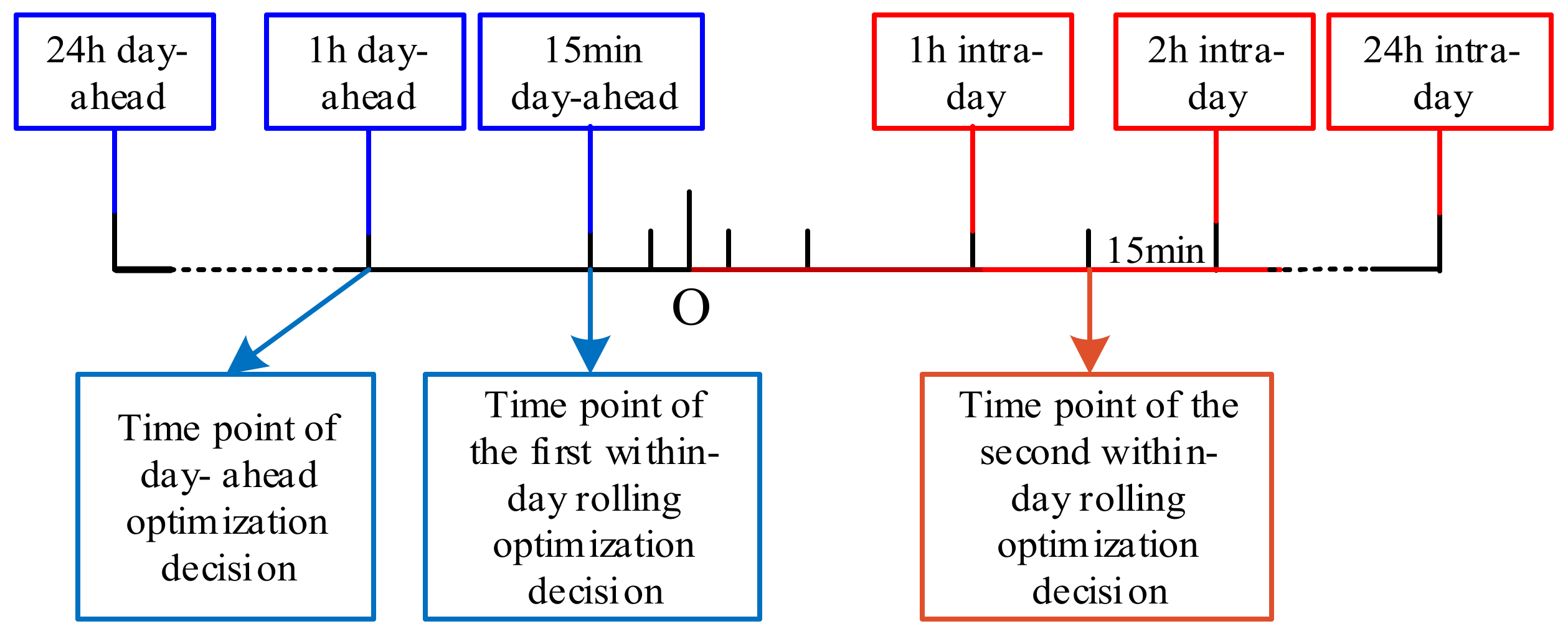
3.2.5. Intra-Day Rolling Optimization Operation Constraints

Energy storage output limits, start-up and shut-down state limits, and electricity, heating, and cooling spinning reserve constraints of the intra-day rolling optimization model are as follows.

• Energy storage output constraints

The rolling optimization will only be conducted in the remaining periods of the day, with the energy storage being fully charged and discharged according to the output generated by the day-ahead scheduling.

$$P_{(\cdot )}(t)=P_{(\cdot )}^{\mathrm{DA}}(t)$$

(56)

where $P_{(\cdot )}^{\mathrm{DA}}(t)$ represents the electrical, heating, and cooling energy storage output of the day-ahead optimal dispatching, respectively, and $P_{(\cdot )}(t)$ represents the electrical, heating, and cooling energy storage output in the rolling stage of the day, respectively.

• Output adjustment constraint

Due to the limited adjustment ability of the equipment output of an IES in a single dispatching period, the output of each equipment in the rolling dispatching stage must be based on the units output obtained from the day-ahead plan, and the actual output should be guaranteed within the allowable adjustment range of the units.

$$\left|P_i(t)-P_i^{\mathrm{DA}}(t)\right|\le P_i^{\mathrm{ad}}$$

(57)

where $P_i^{\mathrm{DA}}(t)$ is the output of equipment i in the day-ahead optimization dispatching stage, $P_i^{}(t)$ is the output of equipment i in the intra-day rolling optimization stage, and $P_i^{\mathrm{ad}}$ is the power adjustment capacity of equipment i.

• Spinning reserve constraints

As a terminal energy supply system, an IES needs to reserve a certain amount of spinning reserve to ensure the reliability of regional energy supply. Due to the large inertia time constant of cold and heat, even if the balance of supply and demand cannot be satisfied in a short time, the safe and stable operation of the system will not be affected. Therefore, it is not necessary to prepare the spinning reserve for cold and heat, and only focus on spinning reserve for electricity. The spinning reserve of an IES can be provided not only by the CCHP unit but also by the internal electrical equipment such as the ER and the HP when the regional multi-energy supply system is equivalent to a virtual power plant.

$$\min \left\{P_{\mathrm{CCHP}}^{\mathrm{ad}},P_{\mathrm{CCHP}}^{\max }-P_{\mathrm{CCHP}}\left(t\right)\right\}+P_{\mathrm{HP}}\left(t\right)+P_{\mathrm{ER}}\left(t\right)+P_{\mathrm{E}}^{\max }-P_{\mathrm{E}}\left(t\right)>=P_{\chi }^{}$$

(58)

where $P_{\chi }^{}$ is the minimum spinning reserve of the regional multi-energy supply system, kW.

• Equipment start-up and shut-down state constraints

In the intra-day rolling dispatching stage, the start-up and shut-down status of a GT and a gas-fired boiler must be the same as the day-ahead optimal scheduling plan.

$$\left\{\begin{array}{l}{u}_{\mathrm{CCHP}}^{}\left(t\right)=u_{\mathrm{CCHP}}^{\mathrm{DA}}\left(t\right)\\ u_{\mathrm{GB}}^{}\left(t\right)=u_{\mathrm{GB}}^{\mathrm{DA}}\left(t\right)\end{array}\right.$$

(59)

where $u_{\mathrm{CCHP}}^{\mathrm{DA}}\left(t\right)$ and $u_{\mathrm{GB}}^{\mathrm{DA}}\left(t\right)$ are, respectively, the start-up and shut-down states of CCHP units and gas-fired boilers in the day-ahead optimal dispatching stage, and $u_{\mathrm{CCHP}}^{}\left(t\right)$ and $u_{\mathrm{GB}}^{}\left(t\right)$ are, respectively, the start-up and shut-down states of CCHP units and gas-fired boilers in the intra-day rolling optimization scheduling stage.

3.3. Optimal Operation Solution Method

To tackle the uncertainty in PV power output, we adopt the robust optimization method for the day-ahead and intra-day operation so that the obtained solution is feasible with any possible realizations of PV power output. The established robust optimization model in general form is as follows:

$$\begin{array}{c}\hfill \underset{x,u}{\min }\underset{w}{\max }C\left(x,u,w\right)\hfill \\ \hfill \begin{array}{c}\mathrm{s}.\mathrm{t}.G\left(x,u,w\right)\le 0\\ x\in X\end{array}\hfill \\ \hfill u\in U\hfill \\ \hfill w\in W\hfill \end{array}$$

(60)

where $C\left(x,u,w\right)$ is the optimization objective; $G\left(x,u,w\right)$ is the constraint; $x$ and $u$ are decision variables, where $x$ represents continuous variables and $u$ represents 0–1 variables; $w$ represents uncertain parameters, such as PV power output; $X$ and $U$ are feasible sets of $x$ and $u$, respectively; and $W$ is the set of $w$. The detailed objective and constraints are established in Section 3 from Equations (20)–(59).

The day-ahead and intra-day collaborative robust optimization of an IES includes continuous variables, 0–1 variables, and nonlinear terms. Among them, the continuous variables are the output of the gas-fired boiler, heat pump, electric refrigeration, and lithium bromide refrigeration of energy stations in the IES; the output of electrical, heating, and cooling energy storage equipment of energy stations; the tie-line power of the electrical grid; the electrical and heating power between energy stations; and the hot-water temperature of energy station nodes; the nonlinear terms exist in the electric output of the CCHP unit, the gas flow and pressure between energy stations, and the voltage and air pressure of energy station nodes; 0–1 variables are the charging and discharging status of energy storage equipment in energy stations and the start-up and shut-down status of CCHP units and gas-fired boilers in energy stations.

The day-ahead and intra-day collaborative robust optimization model for multi-energy stations in an IES is a mixed integer nonlinear programming model with multiple nonlinear variables, as well as quality and inequality constraints. Limited by the current solving technology, the CCHP unit model, power network, and gas network should be linearized by linearization methods so that the optimal operation model becomes a mixed integer linear programming model, which can be easily solved using off-the-shelf solvers.

After piecewise linearization [36,37,40], the output of CCHP units in energy stations and the gas flow and gas pressure between energy stations are expressed by linear variables and 0–1 variables. There are 9696 continuous variables, 3840 0–1 variables, and 1248 nonlinear terms before linearization. In the process of linearization, the nonlinear terms have been eliminated and the number of continuous variables has increased to 17088. For example, the statistics of variables in an IES with five energy stations are shown in

Table 1. Statistical table of variables before and after linearization of a robust optimization model.

Variable Type	Before Linearization	After Linearization
Continuous variable	(5 × 17 + 8) × 96 = 9696	(5 × 26 + 8 + 4 × 10) × 96 = 17,088
0–1 variable	5 × 8 × 96 = 3840	(5 × 18 + 4 × 10) × 96 = 12,480

.

It can be seen from Table 1 that after adopting the piecewise linearization method, the numbers of linear variables and 0–1 variables have increased significantly. The 0–1 variables have increased by 3.25 times, especially. To ensure the accuracy of the model, the number of linearized segments of the CCHP unit and gas pipeline model is large, so the variable number increases greatly.

For the day-ahead and intra-day collaborative robust optimization of an IES, the day-ahead robust optimization needs to be conducted firstly with the time interval as 15 min. In the intra-day operation stage, the CCHP unit and gas-fired boiler start-up and shut-down plans obtained from day-ahead robust optimization are taken as constraints, and the charging and discharging status of the electrical, heating, and cooling multi-energy storage equipment under the day-ahead robust optimization are known. On this basis, intra-day rolling robust optimization is carried out every 2 h according to the latest forecast load and PV output data with the time interval as 5 min. The timescale of each optimization is all the remaining periods of the day.

The time scheme of day-ahead and intra-day collaborative rolling robust optimization of an IES is shown in Figure 7. The day-ahead optimization decision needs to be made 1 h before 00:00 of the next day, and each optimization operation period is 24 h. The intra-day rolling optimization decision scheme needs to be made every 2 hours, with 15 min in advance each time, and each optimization operation time is the total of the remaining periods of the day.

The process of day-ahead and intra-day collaborative robust optimization of an IES is shown in Figure 8, and the specific steps are as follows:

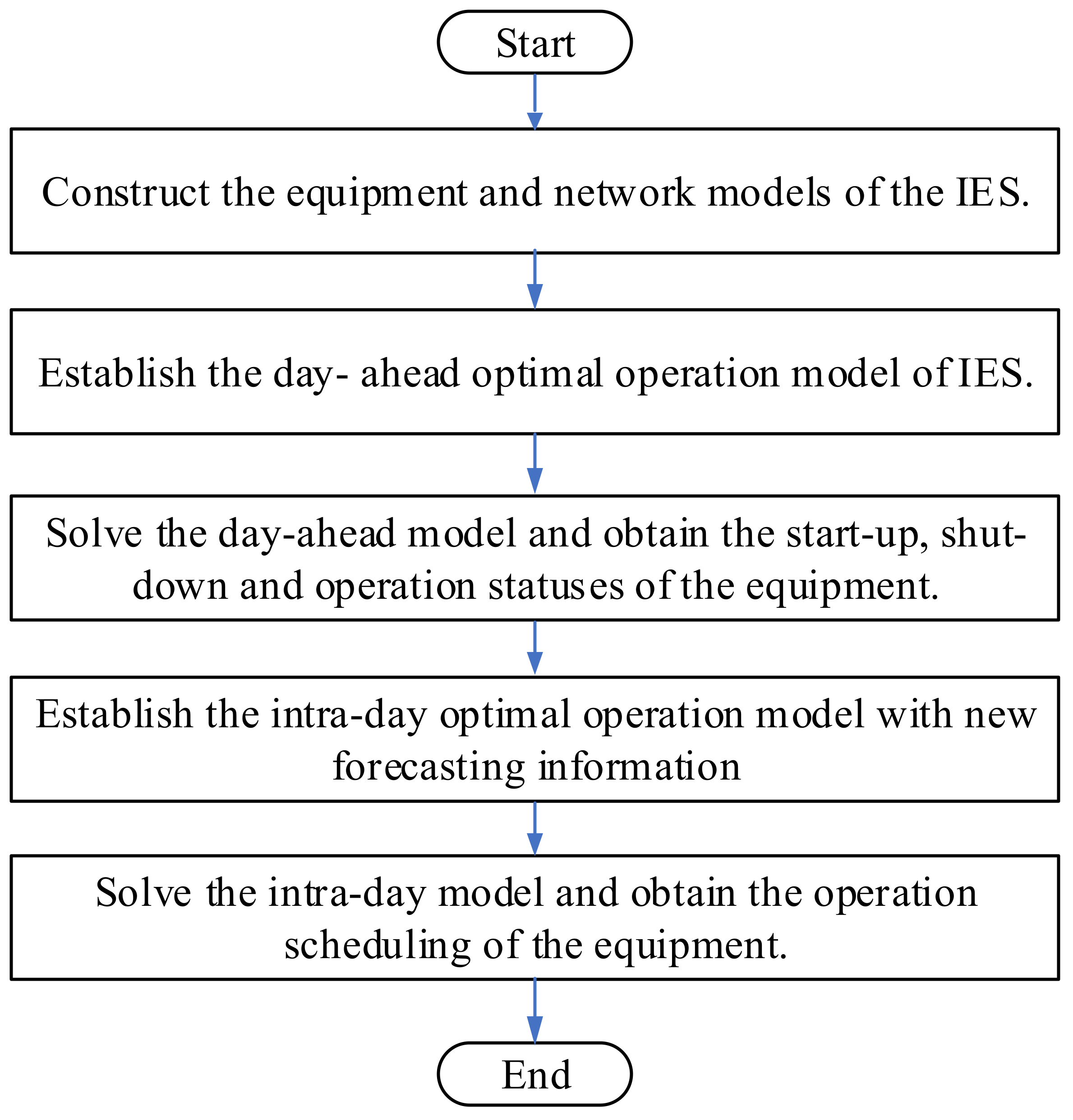
• Step 1: Construct IES network and equipment models based on network construction and equipment parameters.
• Step 2: Establish the day-ahead optimal operation model of the IES with day-ahead PV and load forecast information.
• Step 3: Solve the day-ahead optimal operation model to obtain the start-up, shut-down, and operation status of the unit equipment.
• Step 5: Establish the intra-day collaborative optimization operation model based on day-ahead pre-dispatch results and updated forecasting information.
• Step 6: Solve the intra-day operation model to obtain the operation scheduling of equipment for the subsequent time periods.

4. The Example Analysis

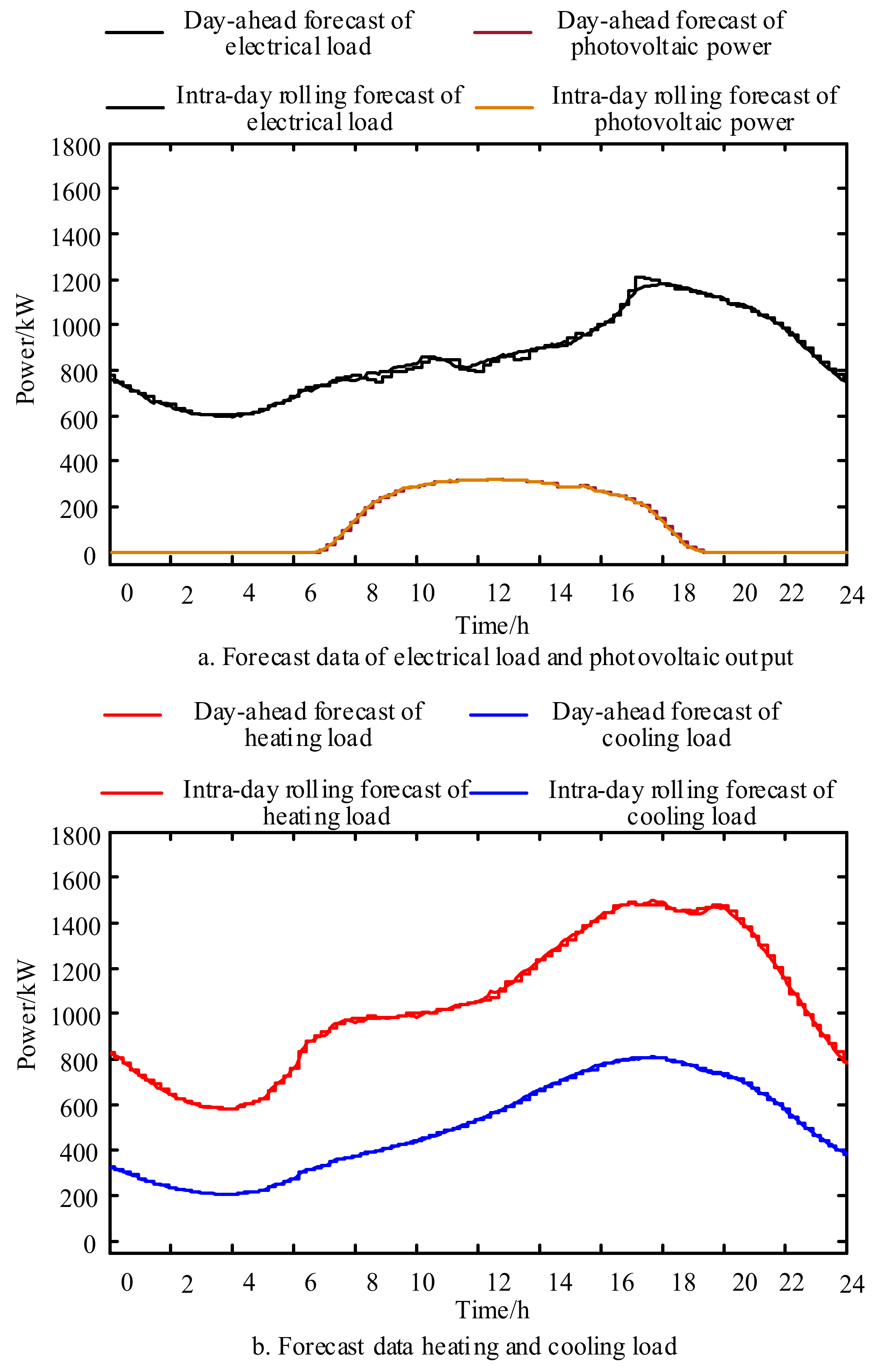
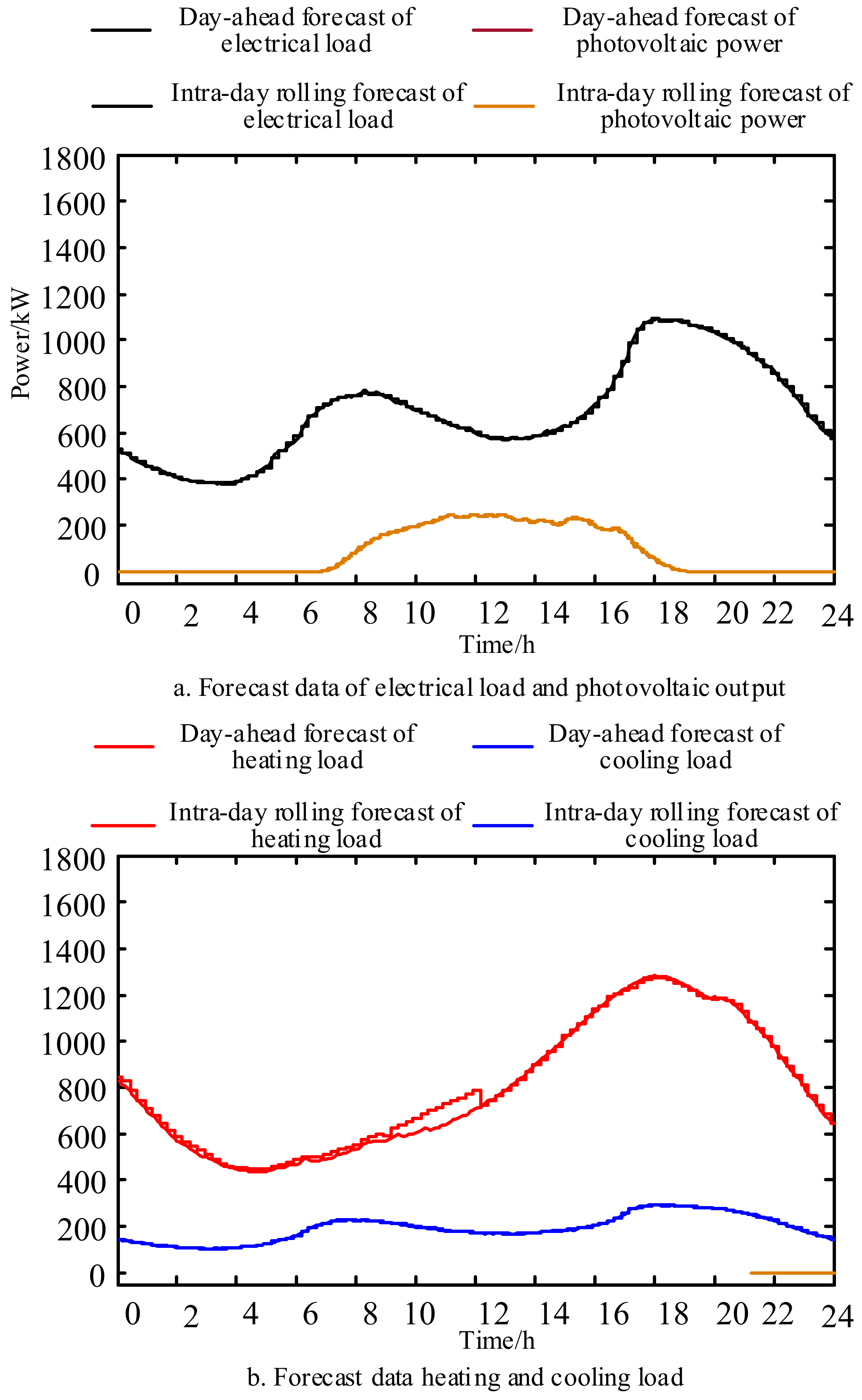
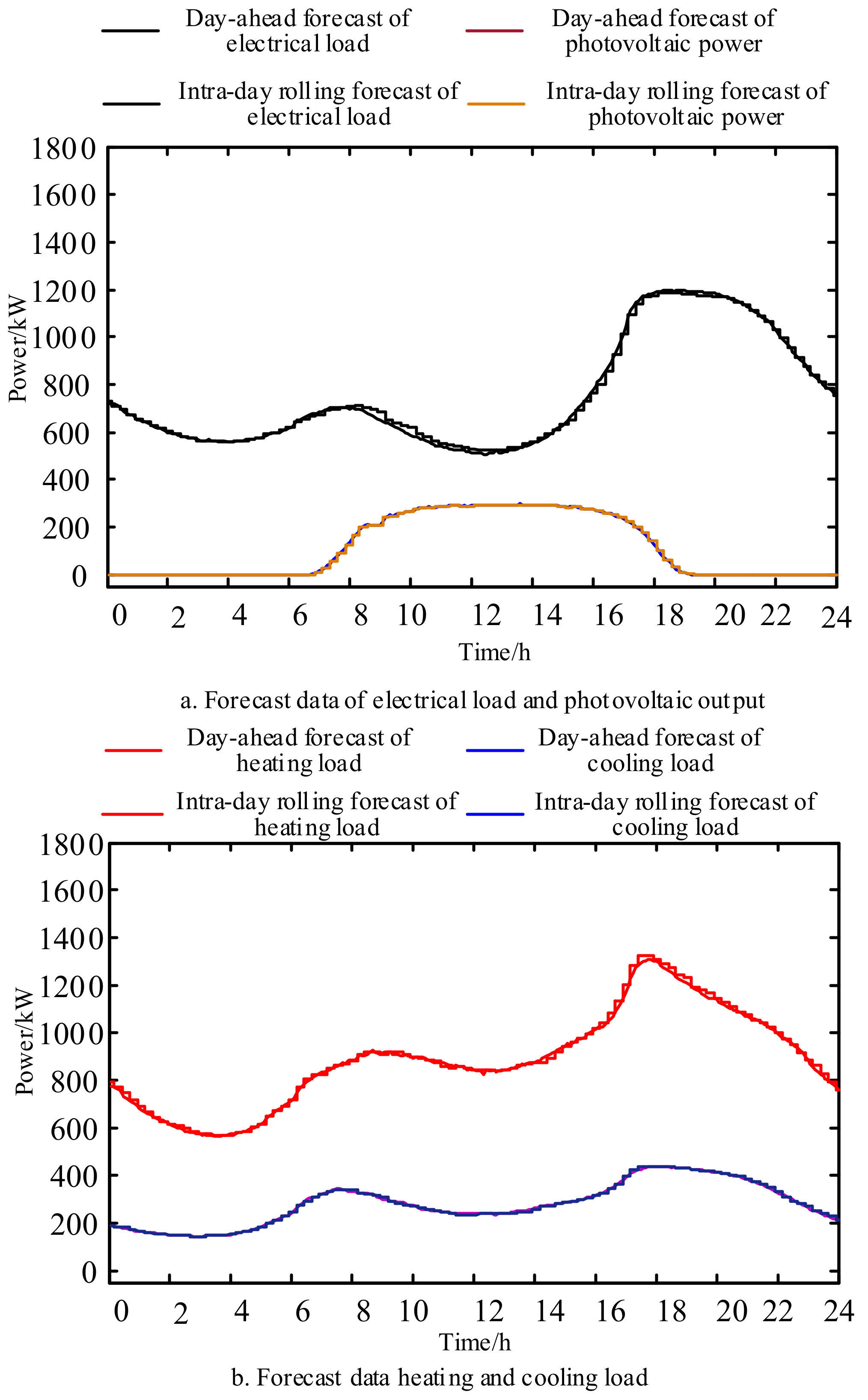
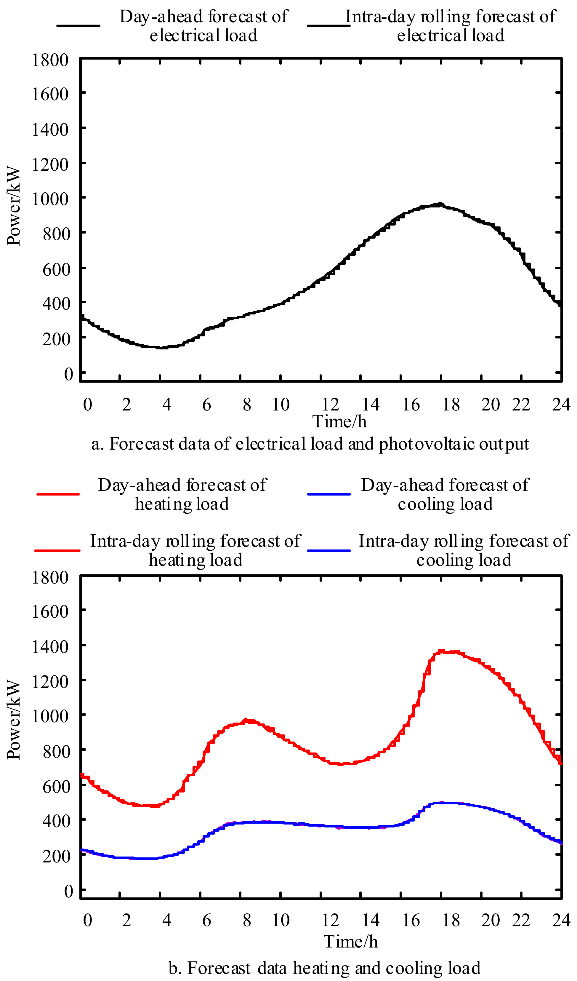
4.1. Example Data

This paper takes a demonstration project as an example, including five energy stations connected to a 10 kV electrical distribution network. The energy flow network of the regional IES is shown in Figure 1. The equipment configuration of the energy station is shown in

Table 2. Energy station equipment configuration.

Equipment	ES1	ES2	ES3	ES4	ES5
Combined cool heat and power (CCHP)	√	√	√	√	√
Gas boiler (GB)	√	√	√	√	×
Electric refrigerator (ER)	√	√	√	√	√
Heat pump (HP)	√	√	√	×	√
Photovoltaic (PV)	√	√	√	×	×
Electric energy storage (ES)	√	√	×	×	×
Heat energy storage (HS)	√	√	×	×	×
Cold energy storage (CS)	√	×	×	√	√

. Taking into account the different load types and PV power generation configurations in different energy stations, the configuration of energy stations in the IES is also different. The electrical and cooling load of energy station 1 is maximal, and it is located in the regional center of the IES. It is also equipped with all energy production conversion and energy storage equipment. Energy stations 4 and 5 are located at the edge of the area and are not equipped with PV power generation, electric energy storage, and thermal energy storage. Energy station 5 is not equipped with a gas boiler, and energy station 4 is not equipped with a heat pump.

The equipment parameters in the energy stations of the IES are shown in

Table 3. The equipment parameters of energy stations.

Equipment		Minimum Power (kW)	Minimum Power (kW)	Up/Down Ramp Rate (kW∙h−1)	Maintenance Cost (CNY∙kW−1)
CCHP	Generation ($P_{\mathrm{CCHP},\mathrm{e}}^{}$)	500	1000	200	0.1
	Waste heat ($P_{\mathrm{CCHP},\mathrm{h}}^{}$)	750	1500	–	–
	Lithium bromide ($P_{\mathrm{CCHP},\mathrm{c}}^{}$)	0	1000	–	0.02
GB ($P_{\mathrm{GB},\mathrm{h}}^{}$)		100	500	100	0012
ER ($P_{\mathrm{ER},\mathrm{e}}^{}$)		0	100	–	0.015
HP ($P_{\mathrm{HP},\mathrm{e}}^{}$)		0	200	–	0.006
PV ($P_{\mathrm{PV},\mathrm{e}}^{}$)		0	400	–	0.0235

and

Table 4. The equipment parameters of energy storage.

Energy Storage	ES	HS	CS
Capacity (kWh)	800	200	200
Maximum charging and discharging ratio	0.2	0.2	0.2
Charging and discharging efficiency	0.90	0.98	0.95
Minimum SOC	0.2	0.2	0.2
Maximum SOC	0.9	0.9	0.9

.

The parameters of power lines, natural gas pipelines, and hot-water pipelines are as shown in

Table 5. Parameters of the pipelines.

Node Number		Line Number	Length (km)
Beginning	End
1	2	1	1
1	3	2	1.5
2	4	3	2
3	5	4	1

. The PV output and load forecast power curves of energy station 1 are shown in Figure 9, and the PV output and load forecast power curves of the other energy stations are shown in the attached pictures in Appendix A.

The electrical impedance per unit length of the power line is 0.0004 + j0.00028 Ω. There are four sections using the same type of transfer lines. The maximum transfer power of the line is 2000 kVA, and its maximum node voltage deviation is ±5%. The coefficient of natural gas pipelines, $C_{ij}^{}$, is 80. The minimum value of pipeline node air pressure is 10 MPa, and the maximum one is 50 MPa. The temperature of the hot-water pipeline drops by 2 °C per kilometer.

4.2. Analysis of Simulation Results

Table 6. The operating results of independent and collaborative optimization operations.

Categories		Independent Operation (CNY)	Collaborative Operation (CNY)
Electrical Cost	Purchasing	6880	5865.7
	Sale	8952	0
	Total	−2072	5865.7
Fuel cost		56,497	38,860
Start-up and shut-down cost		35	9
Maintenance cost		8244	6335.8
Demand response revenue		764	384.1
Total		61,940	50,686

shows a comparison between the results of independent and collaborative optimization operations of five energy stations. The cost of the collaborative optimization operation is 11.254 CNY, which is less than that of the independent operation, and is reduced by 18%. The equipment maintenance cost of the collaborative optimization operation is much lower than that of the independent operation. The start-up and shut-down cost is also less, which indicates that the collaborative optimization operation reduces the maintenance workload of the equipment, as well as start-up and shut-down times. The collaborative optimization operation is more conducive to the operation and maintenance of the equipment. In addition, the increase in the electricity purchase cost and the decrease in the natural gas purchase cost indicate that the collaborative optimization operation benefits the low-carbon environmental protection.

To study the impacts of the electric load participation in the demand response and the uncertainty of PV generation output on the optimal operation of the IES [41], simulation analyses of optimized operation of the IES under different degrees of load demand response participation and the uncertainty of PV generation output are carried out separately.

4.2.1. The Impacts of Demand Response

Simulations of optimized operation of the IES under different levels of load demand response participation are conducted, as shown in Case 1 to Case 5. Note that to guarantee users’ comfort, the demand response participation levels are set relatively small. In

Table 7. The operating results considering different demand respond participations.

Categories		Case 1 (CNY)	Case 2 (CNY)	Case 3 (CNY)	Case 4 (CNY)	Case 5 (CNY)
Electrical Cost	Purchasing	6468.6	6382.9	5448.1	5357.3	5362.6
	Sale	0	0	0	0	0
	Total	6468.6	6382.9	5448.1	5357.3	5362.6
Fuel cost		38,350	38,638	39,440	39,519	39,514
Start-up and shut-down cost		15	15	15	15	6
Maintenance cost		6267.9	6307.1	6416.3	6427.2	6426.5
Demand response revenue		0	0	190.8	384.8	771.9
Total		51,101	51,343	51,129	50,933	50,537

, results in different situations are listed.

• Case 1: The demand response and the uncertainty of PV power generation output are not considered.
• Case 2: The demand response is not considered, and the uncertainty of PV power generation output is 60%.
• Case 3: The demand response participation is 5% of the total electric load, and the uncertainty of the PV output is 60%.
• Case 4: The demand response participation is 10% of the total electric load, and the uncertainty of the PV output is 60%.
• Case 5: The demand response participation is 20% of the total electric load, and the uncertainty of the PV output is 60%.

According to the total expense of the five operating cases shown in Table 7, the cost of Case 2 tops the rank, while the cost of Case 5 is lowest ranked, which indicates that robust optimization will increase the operating expense to allow the IES to ensure the supply of electricity and other energy sources when the PV output deviates from the predicted value. In addition, the higher the demand response participation is, the lower the system operating expense will be. The participation of the power load demand response can offset the growth of the operating expense caused by the uncertainty of the PV output when it reaches a certain percentage. In this paper, only the translational load’s participation in the demand response is taken into consideration. To ensure users’ normal demand and energy comfort, the proportion of translational load to total load must be low. As a result, the reduced operating expense due to that the demand response participation level is relatively smaller.

4.2.2. The Impacts of Uncertainty of PV Power Output

To test the impact of uncertainty of PV on the operation results, another five cases with varying PV uncertainty levels are set and compared. In addition to normal conditions with smaller uncertainty levels, an extreme condition where the day-ahead PV uncertainty reaches 90% is also used to test the robustness of the proposed optimization strategy. Simulation analysis and the optimized operation results are shown in

Table 8. The operating results of different PV output uncertainties.

Categories		Case 1 (CNY)	Case 2 (CNY)	Case 3 (CNY)	Case 4 (CNY)	Case 5 (CNY)
Electrical Cost	Purchasing	6468.6	5865.7	5872.7	5357.3	5477.3
	Sale	0	0	0	0	0
	Total	6468.6	5865.7	5872.7	5357.3	5477.3
Fuel cost		38,350	38,860	38,964	39,519	39,626
Start-up and shut-down cost		15	9	9	15	15
Maintenance cost		6267.9	6335.8	6350.3	6427.2	6442
Demand response revenue		0	384.1	384.5	384.8	385.4
Total		51,101	50,686	50,812	50,933	51,175

.

• Case 1: The uncertainty of the PV output and the demand response are not taken into account.
• Case 2: The uncertainty of the PV output is not considered, while the power load demand response participation rate is 10%.
• Case 3: The uncertainty of the PV output is 30%, and the participation rate of the power load demand response is 10%.
• Case 4: The uncertainty of the PV output is 60%, and the participation rate of the power load demand response is 10%.
• Case 5: The uncertainty of the PV output is 90%, and the participation rate of the power load demand response is 10%.

According to the results in Table 8, we can see that except for Case 1, in which the power load demand response is not considered, from Case 2 to Case 5, the yield of the demand response is basically the same. This manifests that different degrees of the PV output uncertainty barely have an effect on the demand response. In addition, when the participation rate of the demand response is 10%, machine group start-up and shut-down costs under different degrees of the PV output uncertainty are 9 CNY, 15 CNY, 27 CNY, and 15 CNY, respectively. This indicates that PV output uncertainty casts a great influence over the CCHP machine group and start and stop of the gas boiler. The uncertainty of the PV output acts as a guide to working out the day-ahead machine group start and stop plan. In terms of the total expense, the PV output in Case 3 embodies the biggest uncertainty (90%), while the one in Case 2 shows the minimum indeterminacy (0%).

Correspondingly, in Case 3, the operating cost is the highest, while in Case 2, the operating cost is the lowest, with a difference of 489 CNY. In Case 3, compared with the fee of Case 2, the operating cost increases by 1%.

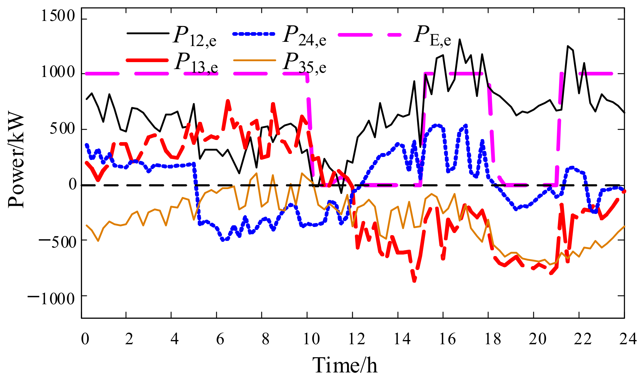
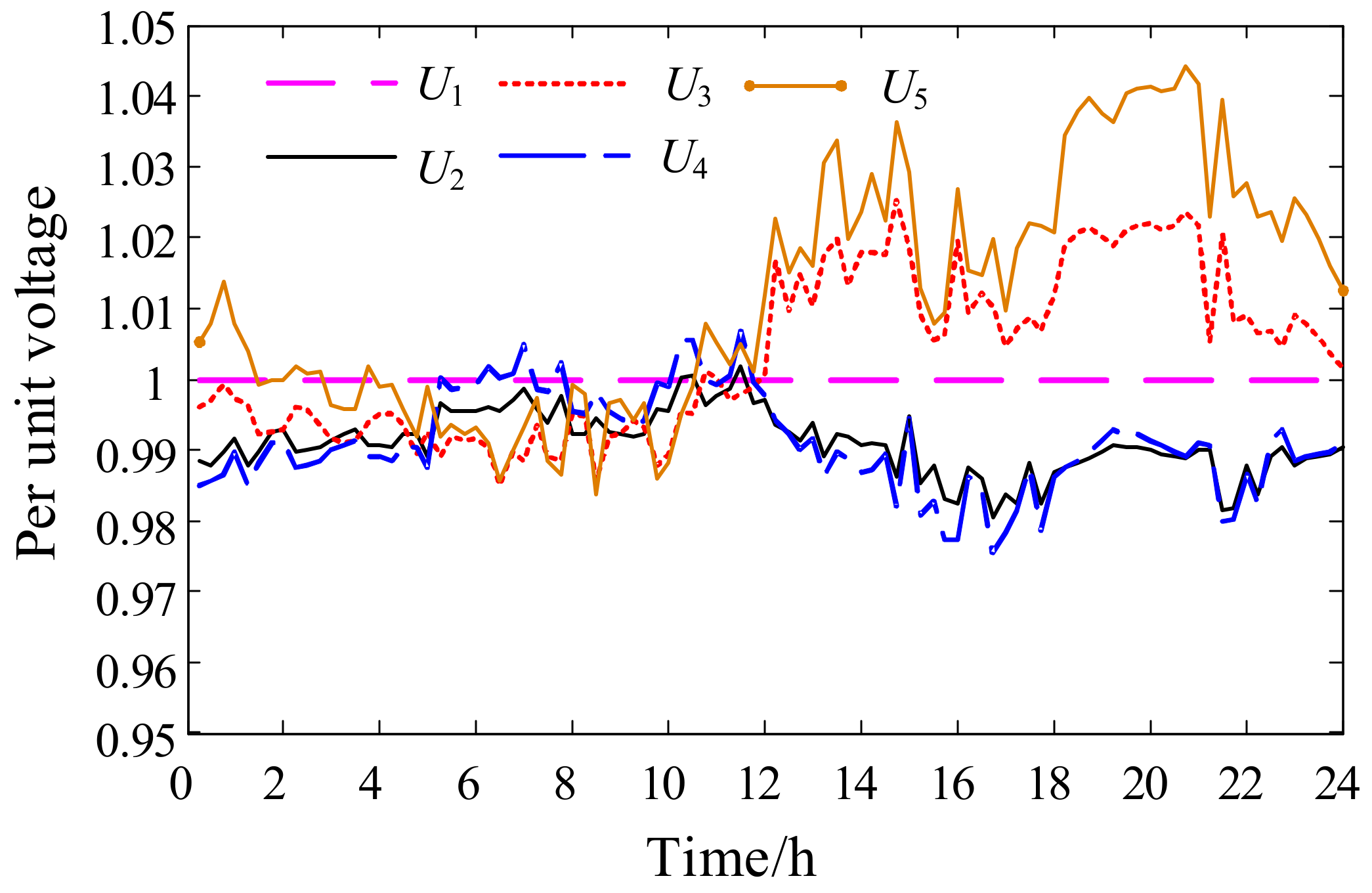
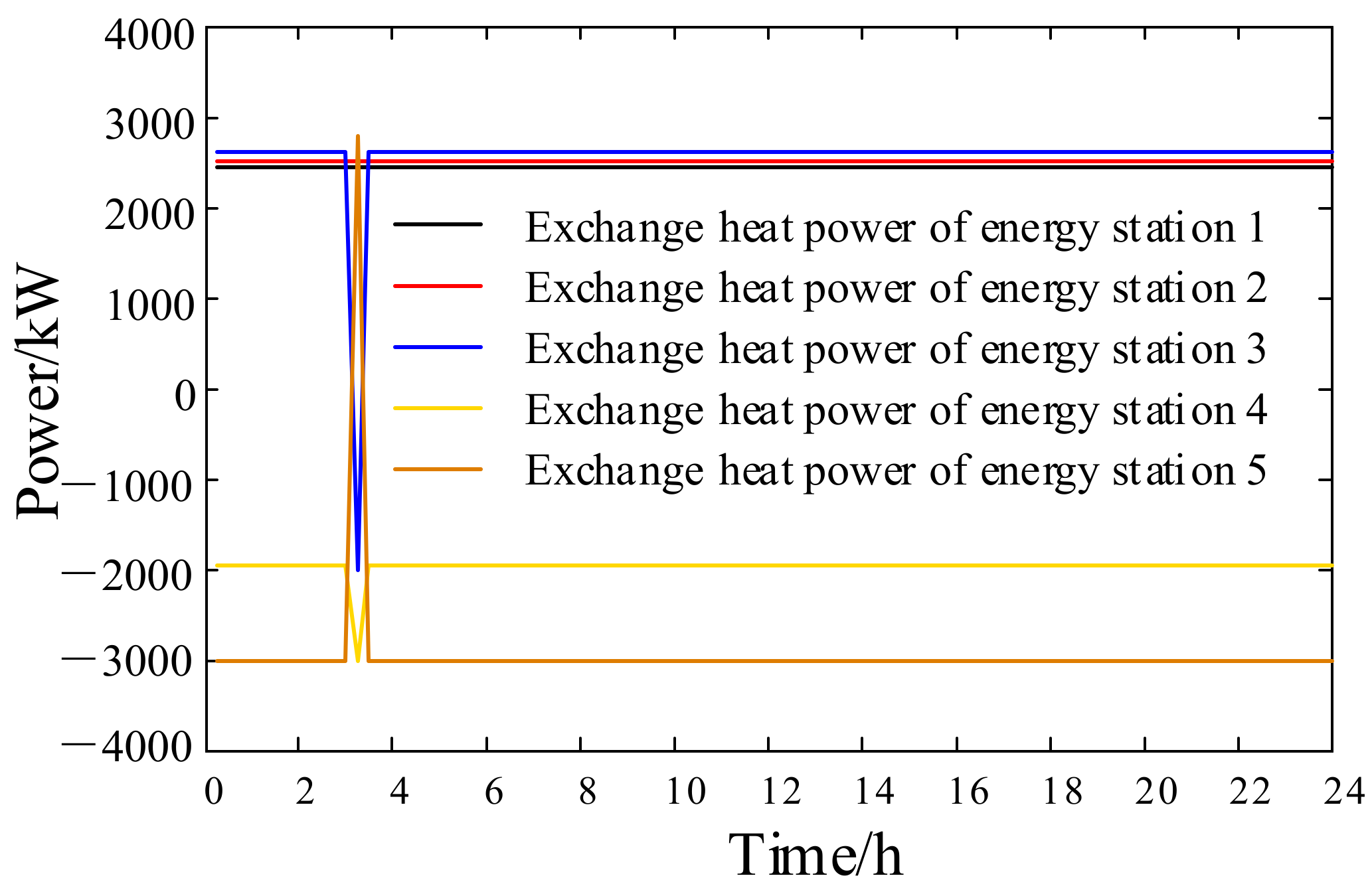
4.2.3. The Operation of Tie-Lines

To study the effect of energy complementarity and energy supply reliability brought by optimal operation, it is necessary to analyze the operation of tie-lines between energy stations.

When the participation degree of the power load demand response is 20% and the uncertainty of the PV output is 60%, the operation of tie-lines between energy stations is shown in Figure 10 and Figure 11, in which $P_{ij,\mathrm{e}}^{}$, $P_{\mathrm{E},\mathrm{e}}^{}$, and $U_i^{}$ have been explained in Equations (11) and (12). To reduce the impact of tie-line capacity, the maximum grid interaction power of the integrated system is ±1000 kVA In Figure 10, it can be clearly seen that with collaborative operation of multiple energy stations, the IES does not send electricity back to the grid, and either it is purchasing electricity from the grid or it is under the condition of neither purchasing nor selling electricity during all operating periods of the day.

Comparing Figure 10 and Figure 11, it can be found that the node voltages of each energy station operate within the operating range (0.95, 1.05). Energy station 1 is located at the node of the power grid and is basically in the state of power output. As for energy station 5, it is located on the edge of the IES and has long been under the state of negative power output, and it only outputs small power for a short time during the peak period of electrovalence. The output power of energy stations 2 and 4 is both positive and negative, which indicates that enhancing the power grid strength between energy stations is conducive to promoting energy complementarity between energy stations and reducing the impact on the power grid.

The power exchange in hot-water pipelines between multi-energy stations in the IES is shown in Figure 12. The power fluctuation of thermal energy flow between energy stations is relatively small, and energy stations 1, 2, and 3 are basically under the state of heat input. Additionally, energy stations 4 and 5 are located on the edge of the IES and are primarily in the stage of power output. There is only a short-term power fluctuation between 3:00 a.m. and 4:00 a.m. The steady transfer characteristic of thermal energy and thermal power coincides with the slow control response of the hot-water pipeline.

According to Figure 12, thermal energy transfer between energy stations is mainly decided by the temperature of the hot water—the heat transfer medium. The temperature of the energy station as the thermal-energy-receiving node is basically 100 °C, which is the upper limit of the temperature constraint. The thermal energy output node is at 50 °C, and this is the lower limit of the hot-water temperature. Since there is a loss of thermal energy during the transfer period in the long-distance pipeline, and the farther the distance is, the greater the loss and the temperature drop will be, the thermal input power of energy station 1 is greater than that of energy station 2. In addition, the energy station 2 heat input power is more than that of station 3.

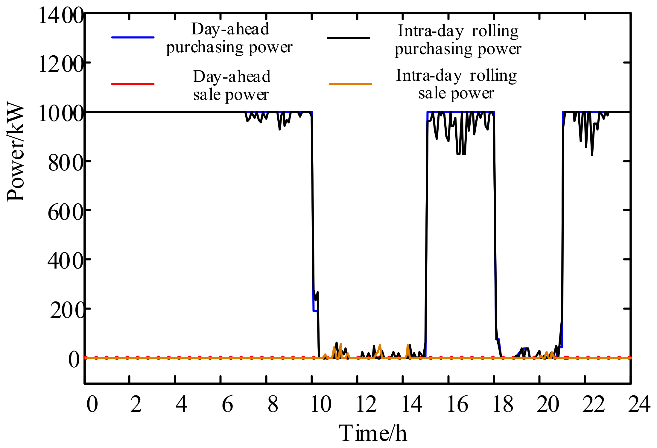
4.2.4. Power Exchange between the Main Grid and the IES

Day-ahead and intra-day operation results are compared and analyzed under the condition that power load demand response participation is 10% and the uncertainty of the PV output is 60%. Figure 13 has clarified the purchase and sale of electricity from the power grid by the IES. It can be observed that the day-ahead sale power from the IES remains 0, meaning that the IES does not sell but only purchases electricity from the power grid during most of the time periods. When the electrovalence reaches its peak, the purchasing power is 0. In most time periods, the IES buys electricity from the power grid during intra-day rolling dispatch, but actually, there are several periods of time where power is sold to the grid. Analyzing the day-ahead and within-day purchasing power, we can clearly find that the former period is more stable and there is almost no fluctuation in tie-line power except the one in the situation of switching from the full power purchase state to the zero power purchase state. However, lots of dense pinnacles come into existence in Figure 13 during day-ahead optimization. This phenomenon indicates that more refined energy optimization management is implemented to trace load fluctuations during the period of with-day rolling operation.

The day-ahead and intra-day optimized power output curves of CCHP units in energy station 1 and energy station 2 are shown in Figure 14. The black line represents the day-ahead optimal scheduling result, and the red one is the intra-day rolling optimal scheduling curve. As we can see in Figure 14, since both the unit dispatching times of intra-day rolling operation and the load prediction power step are 5 min, the power output of the CCHP units fluctuates more smoothly than it has been in the day-ahead one and the amount of output adjustment all fluctuates within the allowable range.

5. Conclusions

Integrated energy systems including several energy stations can realize multi-energy supply of electricity, gas, cold, and heat. In this paper, focusing on the collaborative operation of energy stations, a robust day-ahead and intra-day operation method is proposed, aiming at minimizing the total operation cost. Detailed and comprehensive integrated equipment and energy network constraints are incorporated, and the influence of both the electrical demand response and the uncertainty of the PV output are also taken into account. Further, to make the established optimization model tractable, linearization methods are adopted to convert the optimization model into a mixed-integer linear programming model. A case study on a test system with five energy stations verifies the effectiveness of the proposed method. From case study results, the following conclusions can be drawn: (1) The proposed collaborative operation scheduling strategy helps reduce the total system operating cost via energy exchange among energy stations. Meanwhile, utilization of distributed PV generation can be promoted. (2) The electric load demand response contributes to cost-effective operation results. The higher the demand response participation level is, the more the operation costs are saved. (3) The operation scheduling results are affected by the prediction accuracy of the PV power output. The operating cost grows as the uncertainty level increases.

References

1. Wang, Y.; Wang, X.; Yu, H.; Huang, Y.; Dong, H.; Qi, C.; Baptiste, N. Optimal Design of Integrated Energy System Considering Economics, Autonomy and Carbon Emissions. J. Clean. Prod. 2019, 225, 563–578. [Google Scholar] [CrossRef]
2. Fang, S.; Xu, Y.; Wen, S.; Zhao, T.; Wang, H.; Liu, L. Data-Driven Robust Coordination of Generation and Demand-Side in PV Integrated All-Electric Ship Microgrids. IEEE Trans. Power Syst. 2020, 35, 1783–1795. [Google Scholar] [CrossRef]
3. Cheng, Y.; Zhang, N.; Zhang, B.; Kang, C.; Xi, W.; Feng, M. Low-Carbon Operation of Multiple Energy Systems Based on Energy-Carbon Integrated Prices. IEEE Trans. Smart Grid 2020, 11, 1307–1318. [Google Scholar] [CrossRef]
4. Ponocko, J.; Milanovic, J.V. Multi-objective Demand Side Management at Distribution Network Level in Support of Transmission Network Operation. IEEE Trans. Power Syst. 2020, 35, 1822–1833. [Google Scholar] [CrossRef]
5. Ju, C.; Wang, P.; Goel, L.; Xu, Y. A Two-Layer Energy Management System for Microgrids with Hybrid Energy Storage Considering Degradation Costs. IEEE Trans. Smart Grid 2018, 9, 6047–6057. [Google Scholar] [CrossRef]
6. Pan, Z.; Guo, Q.; Sun, H. Feasible Region Method Based Integrated Heat and Electricity Dispatch Considering Building Thermal Inertia. Appl. Energy 2017, 192, 395–407. [Google Scholar] [CrossRef]
7. Tan, X.; Li, Q.; Wang, H. Advances and Trends of Energy Storage Technology in Microgrid. Int. J. Electr. Power Energy Syst. 2013, 44, 179–191. [Google Scholar] [CrossRef]
8. Teng, Y.; Wang, Z.; Li, Y.; Ma, Q.; Hui, Q.; Li, S. Multi-Energy Storage System Model Based on Electricity Heat and Hydrogen Coordinated Optimization for Power Grid Flexibility. CSEE J. Power Energy Syst. 2019, 5, 266–274. [Google Scholar]
9. Zeng, Z.; Ding, T.; Xu, Y.; Yang, Y.; Dong, Z. Reliability Evaluation for Integrated Power-Gas Systems with Power-to-Gas and Gas Storages. IEEE Trans. Power Syst. 2020, 35, 571–583. [Google Scholar] [CrossRef]
10. Chen, Y.; Wei, W.; Liu, F.; Mei, S. A Multi-Lateral Trading Model for Coupled Gas-Heat-Power Energy Networks. Appl. Energy 2017, 200, 180–191. [Google Scholar] [CrossRef]
11. Fan, F.; Tai, N.; Zheng, X.; Huang, W.; Shi, J. Equalization Strategy for Multi-Battery Energy Storage Systems Using Maximum Consistency Tracking Algorithm of the Conditional Depreciation. IEEE Trans. Energy Convers. 2018, 33, 1242–1254. [Google Scholar] [CrossRef]
12. Chen, X.; Kang, C.; O’Malley, M.; Xia, Q.; Bai, J.; Liu, C.; Sun, R.; Wang, W.; Li, H. Increasing the Flexibility of Combined Heat and Power for Wind Power Integration in China: Modeling and Implications. IEEE Trans. Power Syst. 2015, 30, 1848–1857. [Google Scholar] [CrossRef]
13. Li, J.; Fang, J.; Zeng, Q.; Chen, Z. Optimal Operation of the Integrated Electrical and Heating Systems to Accommodate the Intermittent Renewable Sources. Appl. Energy 2016, 16, 244–254. [Google Scholar] [CrossRef]
14. Zhou, H.; Li, Z.; Zheng, J.H.; Wu, Q.H.; Zhang, H. Robust Scheduling of Integrated Electricity and Heating System Hedging Heating Network Uncertainties. IEEE Trans. Smart Grid 2020, 11, 1543–1555. [Google Scholar] [CrossRef]
15. Liu, G.; Starke, M.; Xiao, B.; Zhang, X.; Tomsovic, K. Microgrid Optimal Scheduling with Chance-Constrained Islanding Capability. Electr. Power Syst. Res. 2017, 145, 197–206. [Google Scholar] [CrossRef] [Green Version]
16. Peng, C.; Hou, Y.; Yu, N.; Wang, W. Risk-Limiting Unit Commitment in Smart Grid with Intelligent Periphery. IEEE Trans. Power Syst. 2017, 32, 4696–4707. [Google Scholar] [CrossRef]
17. Mieth, R.; Dvorkin, Y. Distribution Electricity Pricing under Uncertainty. IEEE Trans. Power Syst. 2020, 35, 2325–2338. [Google Scholar] [CrossRef] [Green Version]
18. Wang, B.; Dehghanian, P.; Zhao, D. Chance-Constrained Energy Management System for Power Grids with High Proliferation of Renewables and Electric Vehicles. IEEE Trans. Smart Grid 2020, 11, 2324–2336. [Google Scholar] [CrossRef]
19. Baringo, L.; Conejo, A.J. Offering Strategy of Wind-Power Producer: A Multi-Stage Risk-Constrained Approach. IEEE Trans. Power Syst. 2016, 31, 1420–1429. [Google Scholar] [CrossRef]
20. Wang, J.; Zhong, H.; Xia, Q.; Kang, C.; Du, E. Optimal Joint-Dispatch of Energy and Reserve for CCHP-Based Microgrids. IET Gener. Transm. Distrib. 2017, 11, 785–794. [Google Scholar] [CrossRef]
21. Pazouki, S.; Haghifam, M.R.; Moser, A. Uncertainty Modeling in Optimal Operation of Energy Hub in Presence of Wind, Storage and Demand Response. Int. J. Electr. Power Energy Syst. 2014, 61, 335–345. [Google Scholar] [CrossRef]
22. Moreira, A.; Street, A.; Arroyo, J.M. An Adjustable Robust Optimization Approach for Contingency- Constrained Transmission Expansion Planning. IEEE Trans. Power Syst. 2015, 30, 2013–2022. [Google Scholar] [CrossRef]
23. Baringo, L.; Baringo, A. A Stochastic Adaptive Robust Optimization Approach for the Generation and Transmission Expansion Planning. IEEE Trans. Power Syst. 2018, 33, 792–802. [Google Scholar] [CrossRef]
24. Wu, H.; Krad, I.; Florita, A.; Hodge, B.M.; Ibanez, E.; Zhang, J.; Ela, E. Stochastic Multi-Timescale Power System Operations with Variable Wind Generation. IEEE Trans. Power Syst. 2016, 32, 3325–3337. [Google Scholar] [CrossRef]
25. Rong, S.; Li, Z.; Li, W. Investigation of the Promotion of Wind Power Consumption Using the Thermal-Electric Decoupling Techniques. Energies 2015, 8, 8613–8629. [Google Scholar] [CrossRef] [Green Version]
26. Li, Z.; Wu, W.; Wang, J.; Zhang, B.; Zheng, T. Transmission-Constrained Unit Commitment Considering Combined Electricity and District Heating Networks. IEEE Trans. Sustain. Energy 2016, 7, 480–492. [Google Scholar] [CrossRef]
27. Li, Z.; Wu, W.; Shahidehpour, M.; Wang, J.; Zhang, B. Combined Heat and Power Dispatch Considering Pipeline Energy Storage of District Heating Network. IEEE Trans. Sustain. Energy 2016, 7, 12–22. [Google Scholar] [CrossRef]
28. Shao, C.; Wang, X.; Shahidehpour, M.; Wang, X.; Wang, B. A MILP-based Optimal Power Flow in Multicarrier Energy Systems. IEEE Trans. Sustain. Energy 2017, 8, 239–248. [Google Scholar] [CrossRef]
29. Wu, C.; Gu, W.; Jiang, P.; Li, Z.; Cai, H.; Li, B. Combined Economic Dispatch Considering the Time-Delay of A District Heating Network and Multi-Regional Indoor Temperature Control. IEEE Trans. Sustain. Energy 2018, 9, 118–127. [Google Scholar] [CrossRef]
30. Duquette, J.; Rowe, A.; Wild, P. Thermal Performance of A Steady State Physical Pipe Model for simulating District Heating Grids with Variable Flow. Appl. Energy 2016, 178, 383–393. [Google Scholar] [CrossRef]
31. Lu, S.; Gu, W.; Meng, K.; Yao, S.; Liu, B.; Dong, Z.Y. Thermal Inertial Aggregation Model for Integrated Energy Systems. IEEE Trans. Power Syst. 2020, 35, 2374–2387. [Google Scholar] [CrossRef]
32. Yang, H.; Zhang, J.; Qiu, J.; Zhang, S.; Lai, M.; Dong, Z.Y. Practical Pricing Approach to Smart Grid Demand Response Based on Load Classification. IEEE Trans. Smart Grid 2017, 9, 179–190. [Google Scholar] [CrossRef]
33. Geramifar, H.; Shahabi, M.; Barforoshi, T. Coordination of Energy Storage Systems and Demand Response Resources for Optimal Scheduling of Microgrids under Uncertainties. IET Renew. Power Gener. 2017, 11, 377–388. [Google Scholar] [CrossRef]
34. Nguyen, D.T.; Le, L.B. Joint Optimization of Electric Vehicle and Home Energy Scheduling Considering User Comfort Preference. IEEE Trans. Smart Grid 2014, 5, 188–199. [Google Scholar] [CrossRef]
35. Tabar, V.S.; Jirdehi, M.A.; Hemmati, R. Energy Management in Microgrid Based on the Multi Objective Stochastic Programming Incorporating Portable Renewable Energy Resource as Demand Response Option. Energy 2017, 118, 827–839. [Google Scholar] [CrossRef]
36. Lei, S.; Hou, Y.; Qiu, F.; Yan, J. Identification of Critical Switches for Integrating Renewable Distributed Generation by Dynamic Network Reconfiguration. IEEE Trans. Sustain. Energy 2018, 9, 420–432. [Google Scholar] [CrossRef]
37. Wang, C.; Wang, Z.; Hou, Y.; Ma, K. Dynamic Game-Based Maintenance Scheduling of Integrated Electric and Natural Gas Grids with A Bilevel Approach. IEEE Trans. Power Syst. 2018, 33, 4958–4971. [Google Scholar] [CrossRef] [Green Version]
38. Alipour, M.; Zare, K.; Mohammadi-Ivatloo, B. Short-Term Scheduling of Combined Heat and Power Generation Units in the Presence of Demand Response Programs. Energy 2014, 71, 289–301. [Google Scholar] [CrossRef]
39. Cheng, Y.; Zhang, P.; Liu, X. Collaborative Autonomous Optimization of Interconnected Multi-Energy Systems with Two-Stage Transactive Control Framework. Energies 2019, 13, 1. [Google Scholar] [CrossRef] [Green Version]
40. Zhang, Y.; Hu, Y.; Ma, J.; Bie, Z. A Mixed-Integer Linear Programming Approach to Security-Constrained Co-Optimization Expansion Planning of Natural Gas and Electricity Transmission Systems. IEEE Trans. Power Syst. 2018, 33, 6368–6378. [Google Scholar] [CrossRef]
41. Zhai, J.; Wu, X.; Zhu, S.; Yang, B.; Liu, H. Optimization of Integrated Energy System Considering Photovoltaic Uncertainty and Multi-Energy Network. IEEE Access 2020, 8, 141558–141568. [Google Scholar] [CrossRef]
Figure 1. Energy flow network of an integrated energy system (IES).
Energies 14 00936 g001
Figure 2. Topological structure diagram of internal equipment in energy station 1.
Energies 14 00936 g002
Figure 3. Energy conversion diagram of combined cool heat and power (CCHP).
Energies 14 00936 g003
Figure 4. Electrical power network topology with energy stations.
Energies 14 00936 g004
Figure 5. Natural gas network topology with energy stations.
Energies 14 00936 g005
Figure 6. Pipe network diagram of a heating supply system.
Energies 14 00936 g006
Figure 7. The decision time scheme of day-ahead and intra-day rolling robust optimization.
Energies 14 00936 g007
Figure 8. Flowchart of day-ahead and intra-day collaborative optimization of an IES.
Energies 14 00936 g008
Figure 9. The day-ahead and intra-day forecast curves of PV and load output of the energy station 1.
Energies 14 00936 g009
Figure 10. Electrical power exchange between multi-energy stations in the IES.
Energies 14 00936 g010
Figure 11. Voltage of energy stations in the IES.
Energies 14 00936 g011
Figure 12. Transfer power of hot-water pipelines between multi-energy stations in the IES.
Energies 14 00936 g012
Figure 13. Electrical power exchange between the main grid and the IES in day-ahead and intra-day optimization.
Energies 14 00936 g013
Figure 14. Day-ahead and intra-day optimized power output curves of CCHP units in the IES.
Energies 14 00936 g014