Three-Dimensional Modeling and Fluid Flow Simulation for the Quantitative Description of Permeability Anisotropy in Tidal Flat Carbonate


Abstract
:
1. Introduction
2. Study Area and Geological Background
3. Data
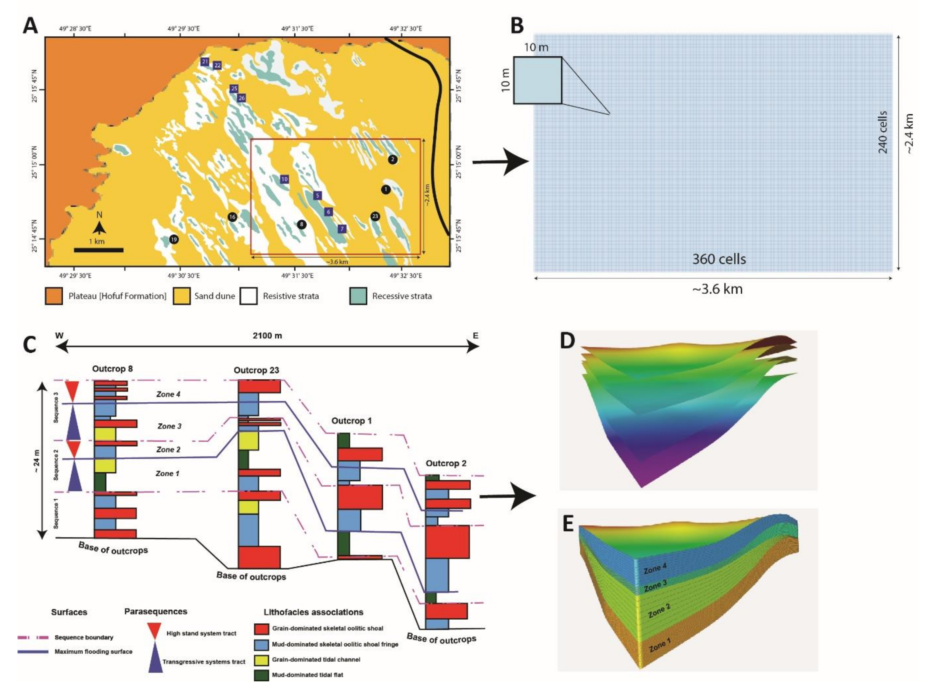
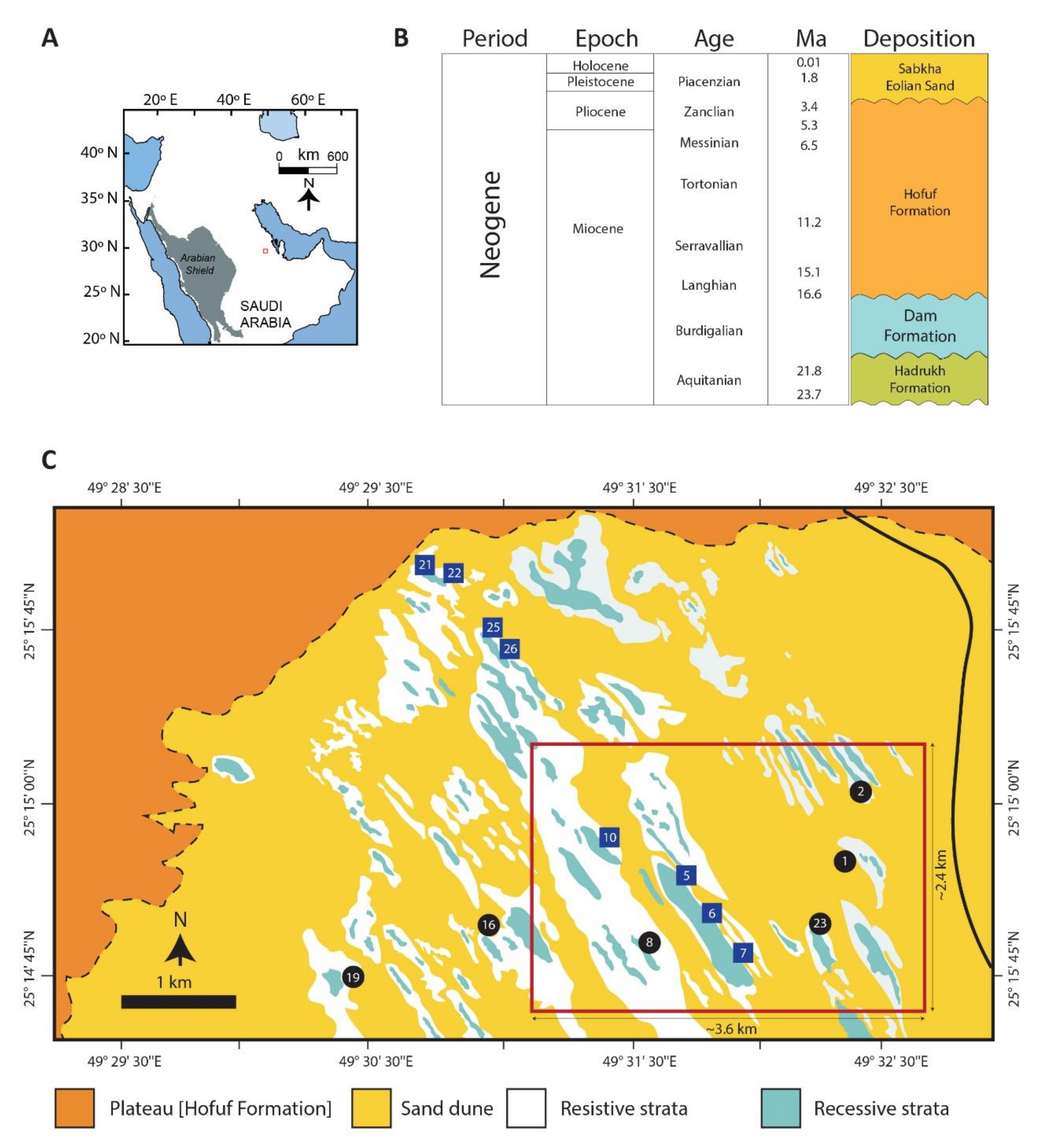
3.1. Location
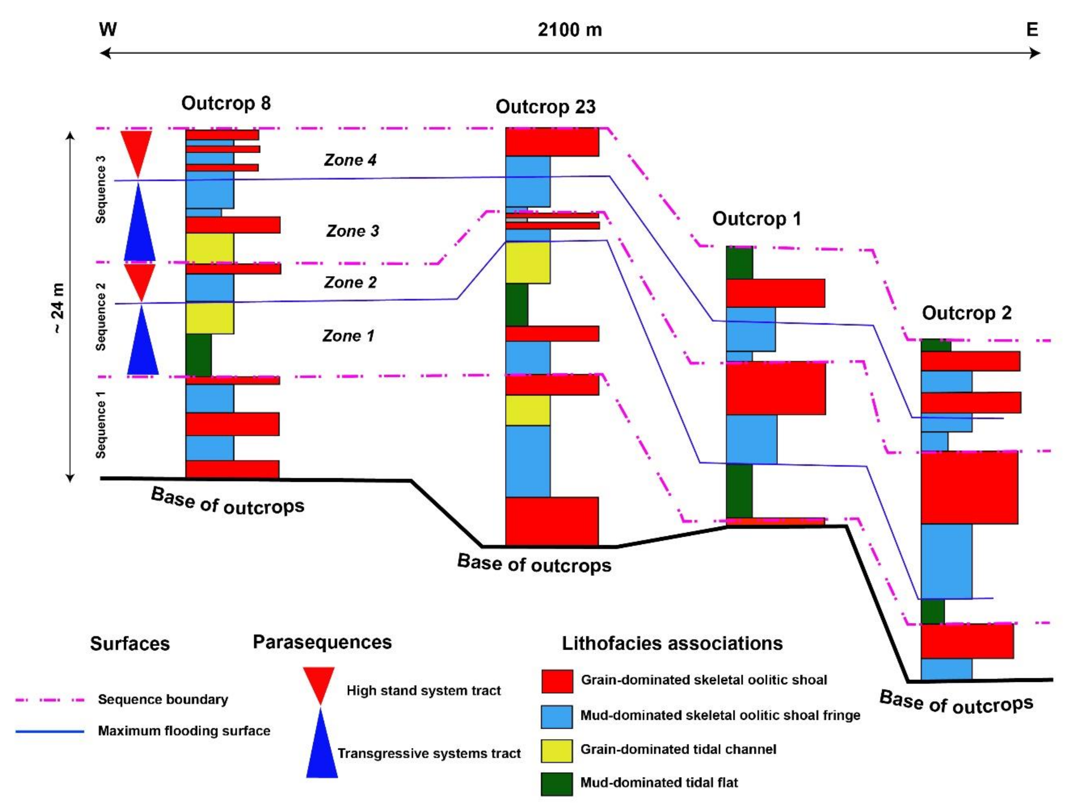
3.2. Stratigraphy
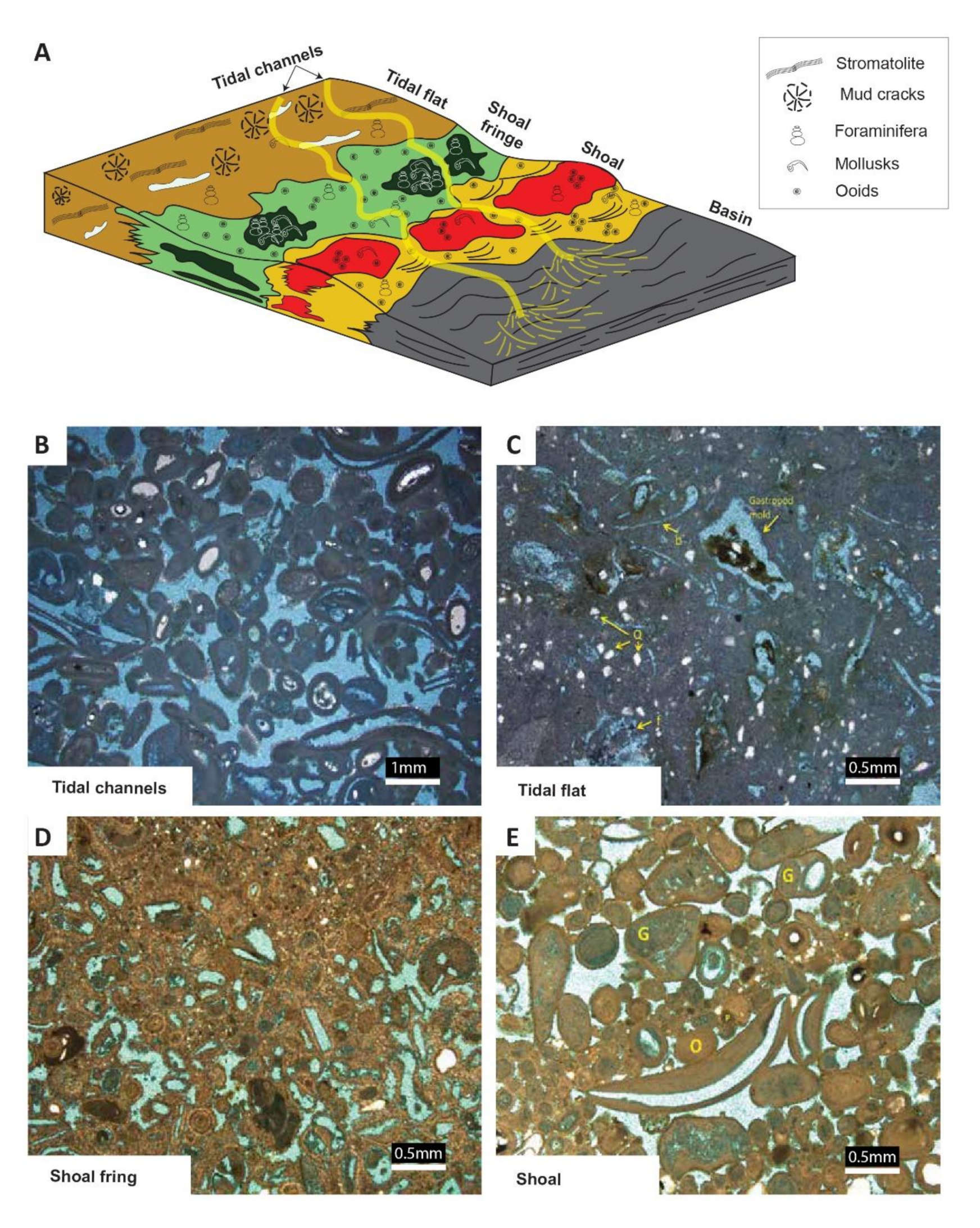
3.3. Lithology
3.4. Petrophysics
3.5. Conceptual Model
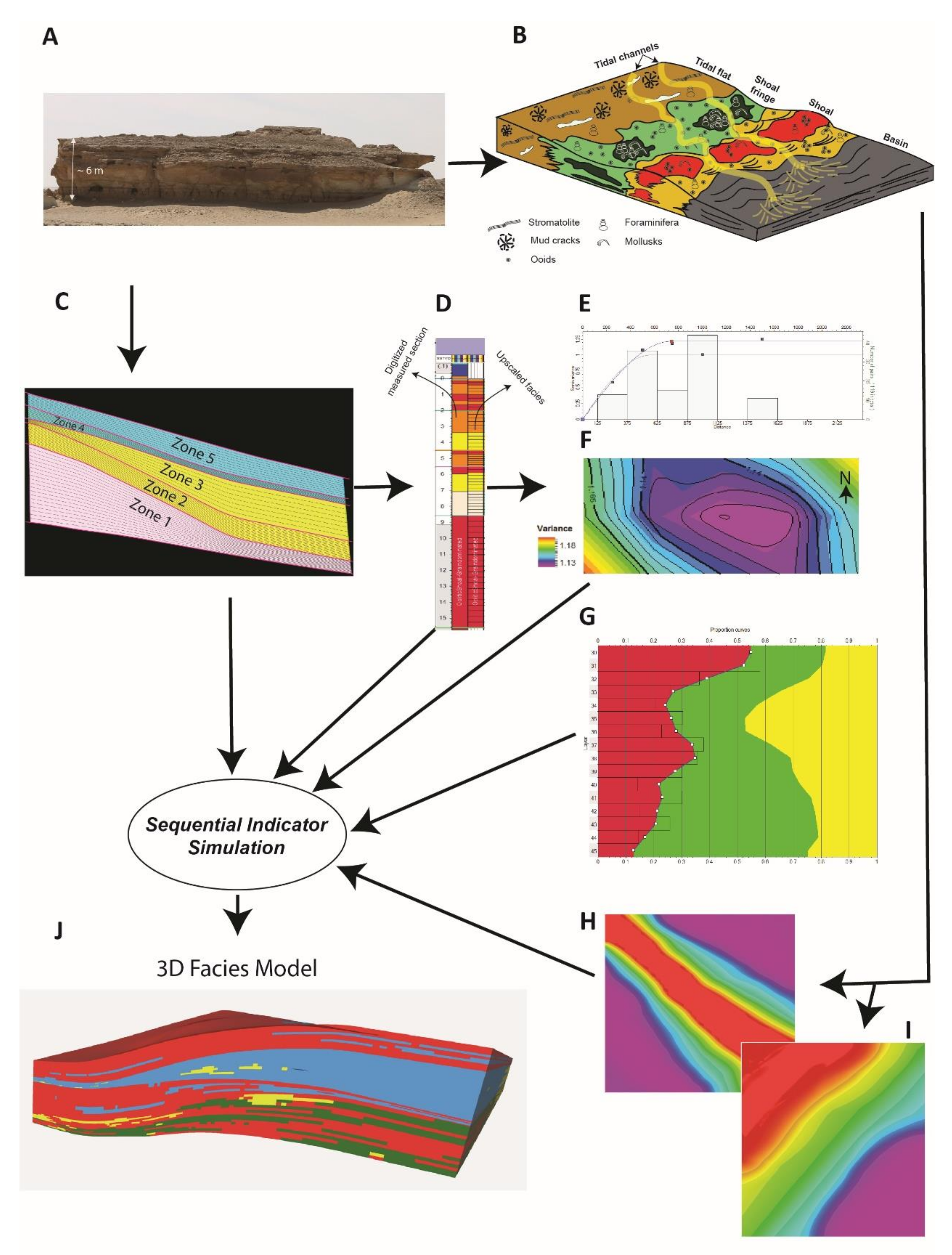
4. Workflow
4.1. Generating the 3D Structure Grid
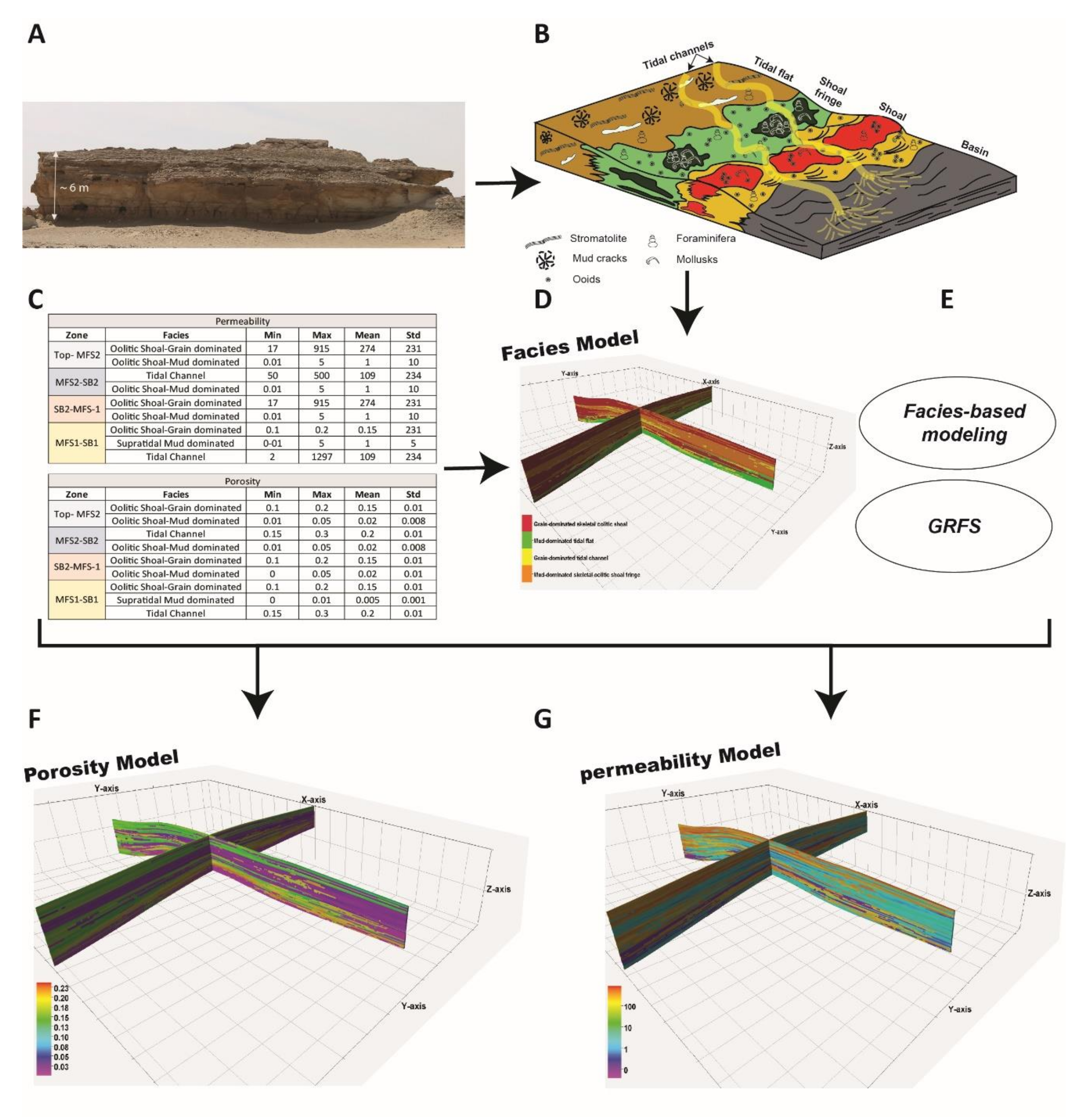
4.2. Generating the 3D Facies Model
4.3. Generating the 3D Property Model
4.4. Generate Upscaled Models
4.5. Fluid Flow Simulation
5. Results
5.1. Analysis of the Data
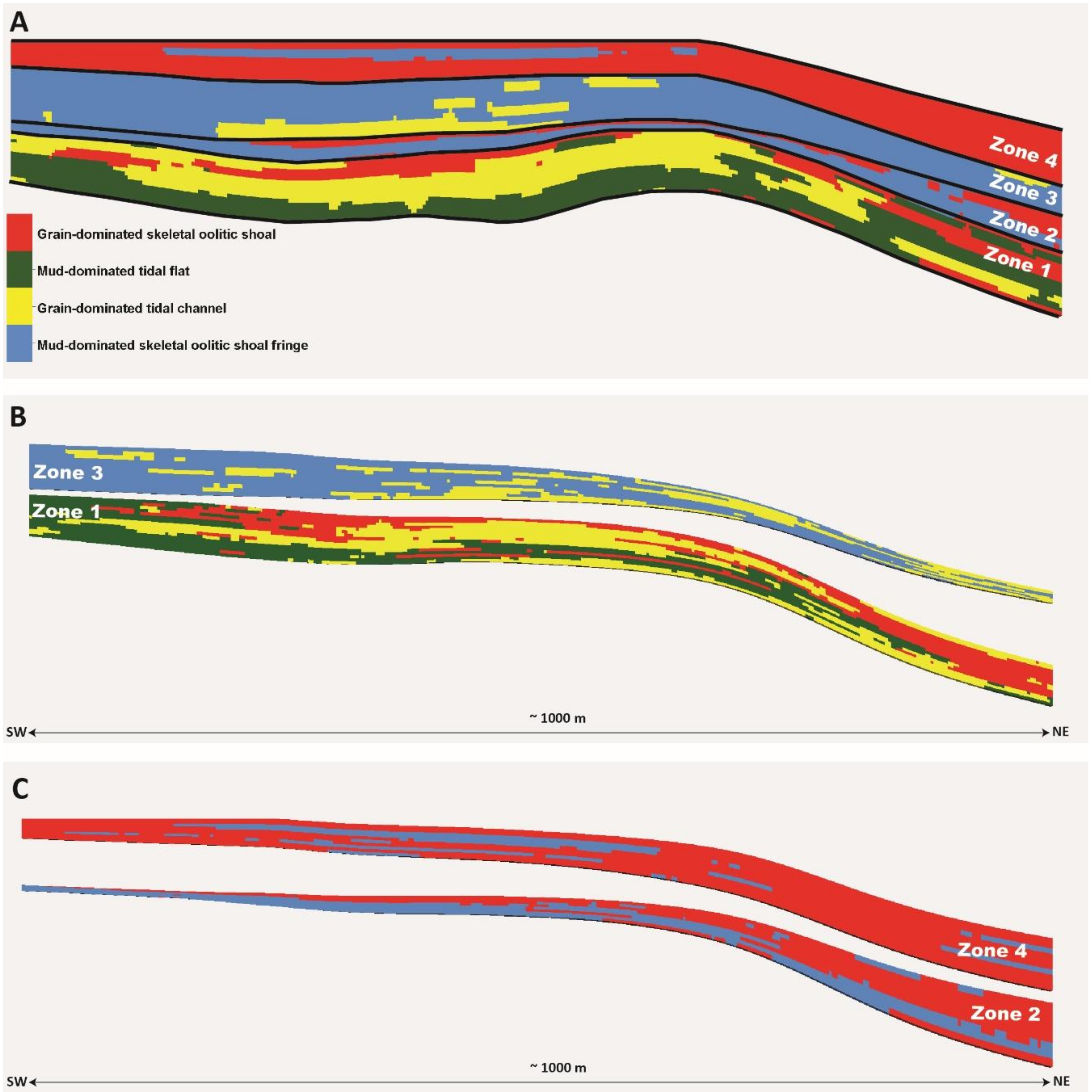
5.2. Distribution of the Lithofacies
5.2.1. Zone 1
5.2.2. Zone 2
5.2.3. Zone 3
5.2.4. Zone 4
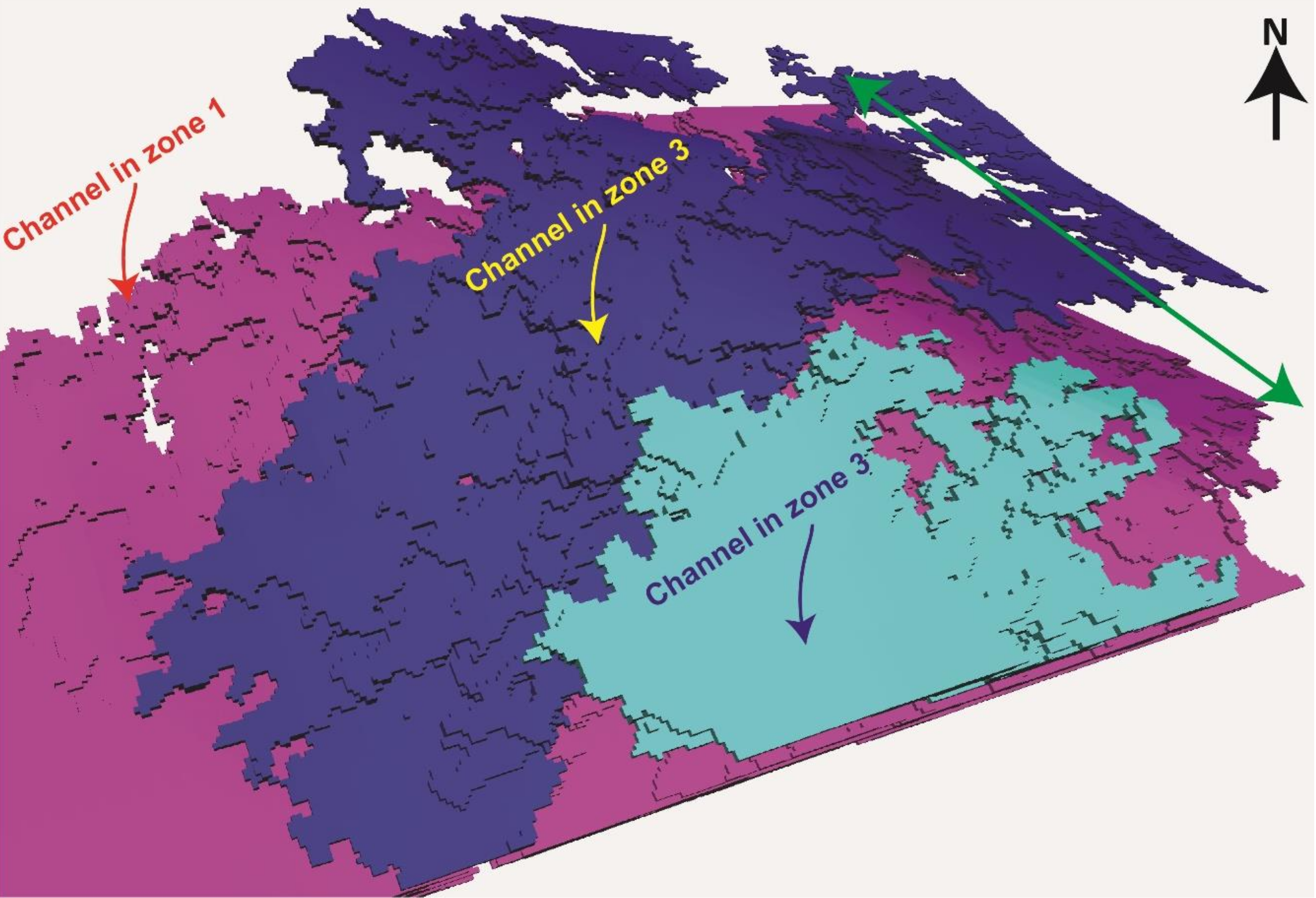
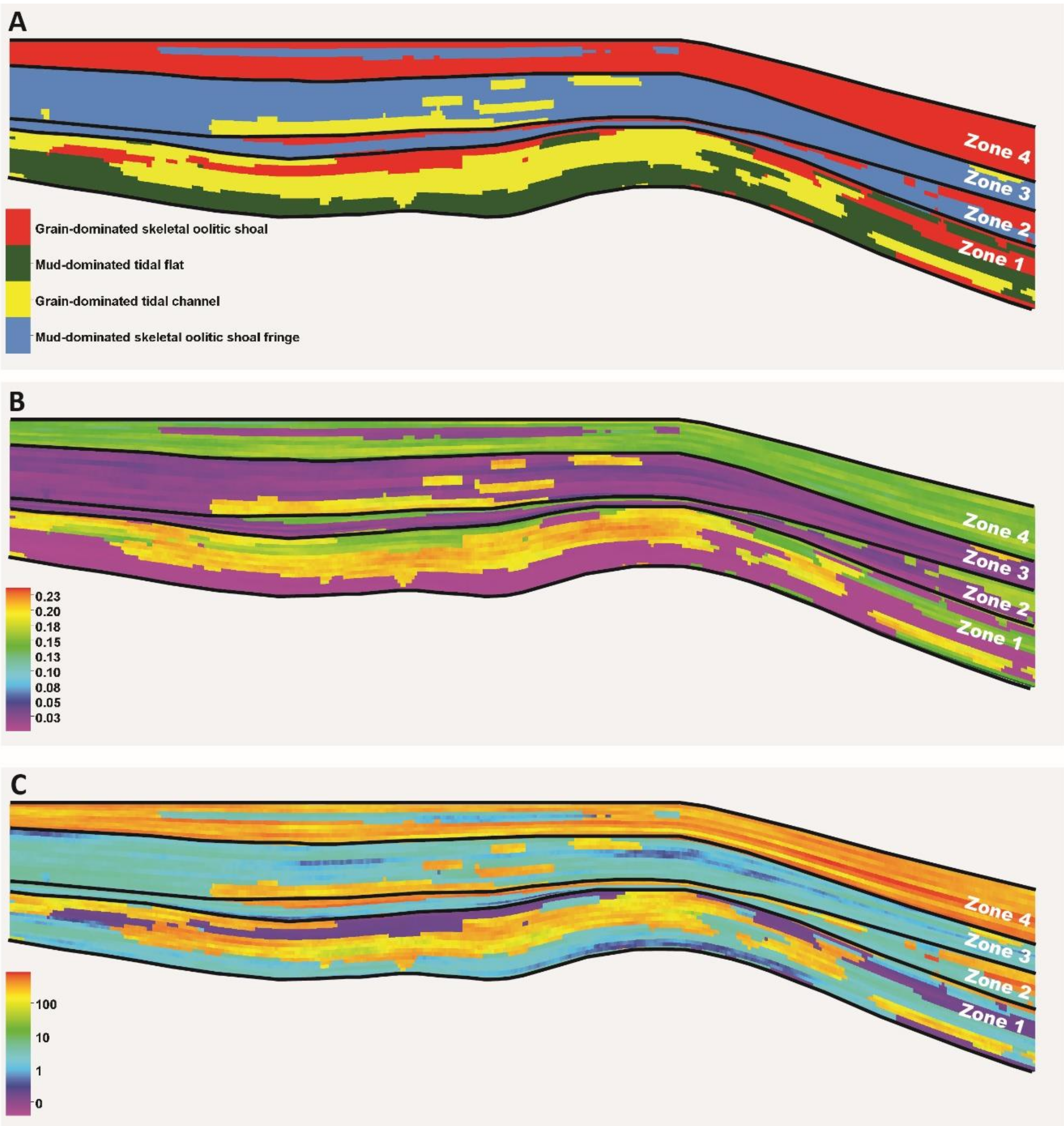
5.3. Architecture of the Lithofacies
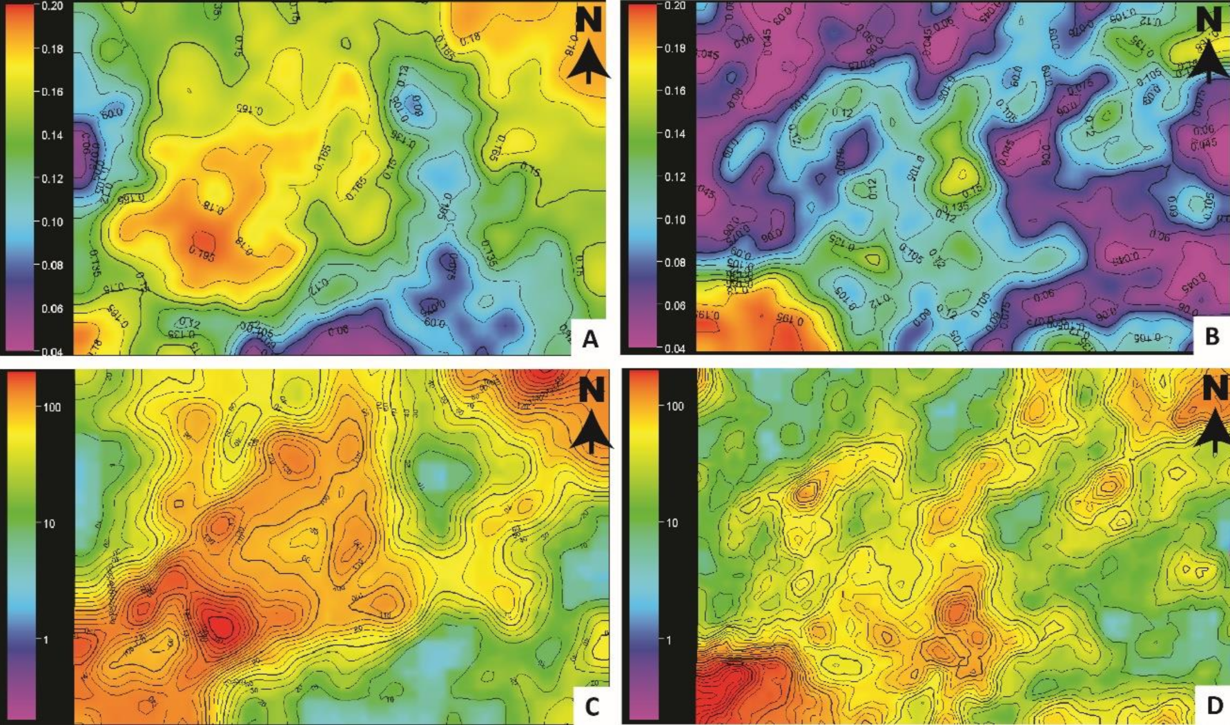
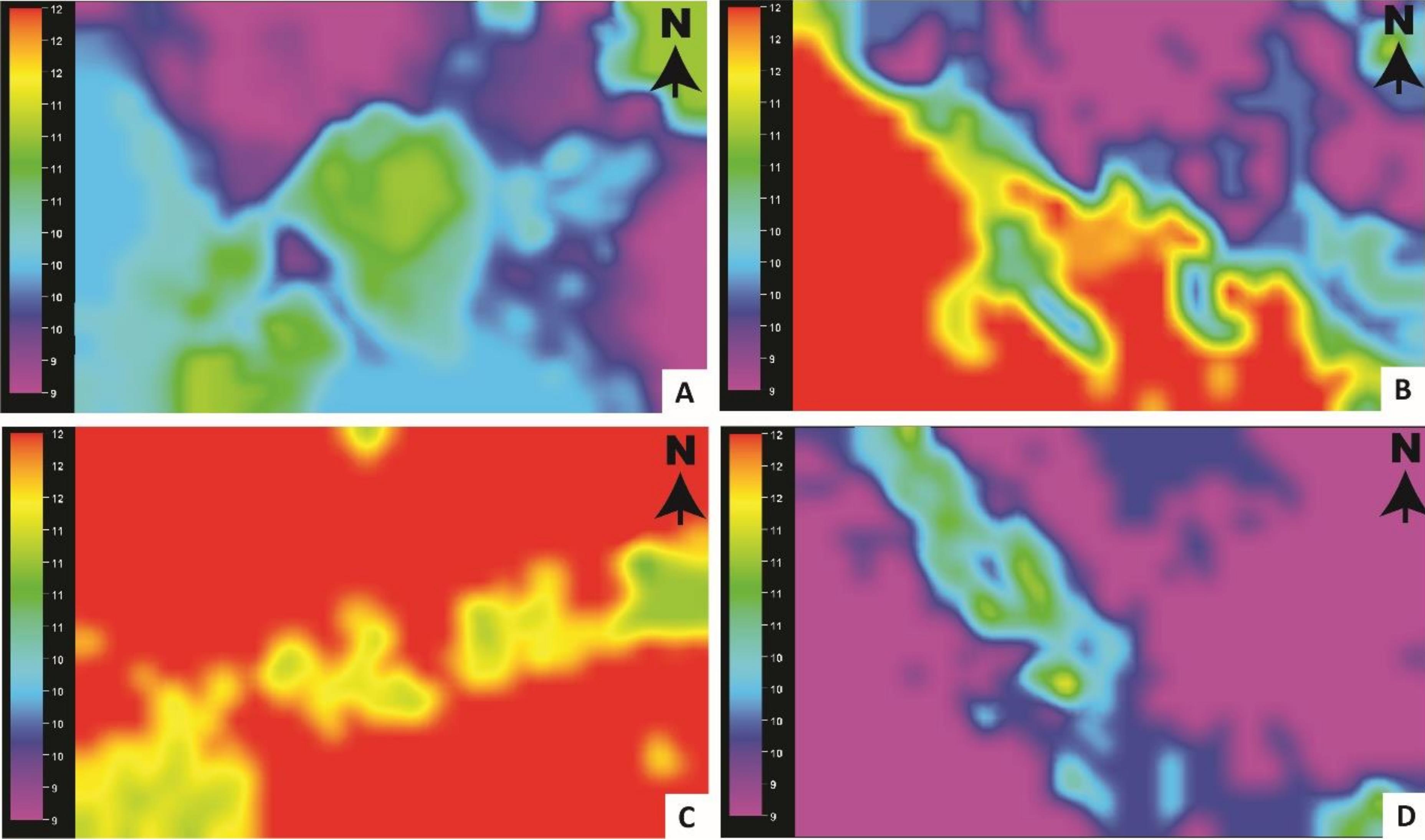
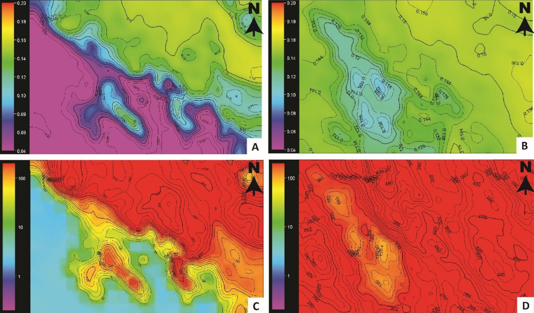
5.4. Trends in Petrophysical Properties
5.5. Trends in Fluid Flow Behavior
5.5.1. First Transect
5.5.2. Second Transect
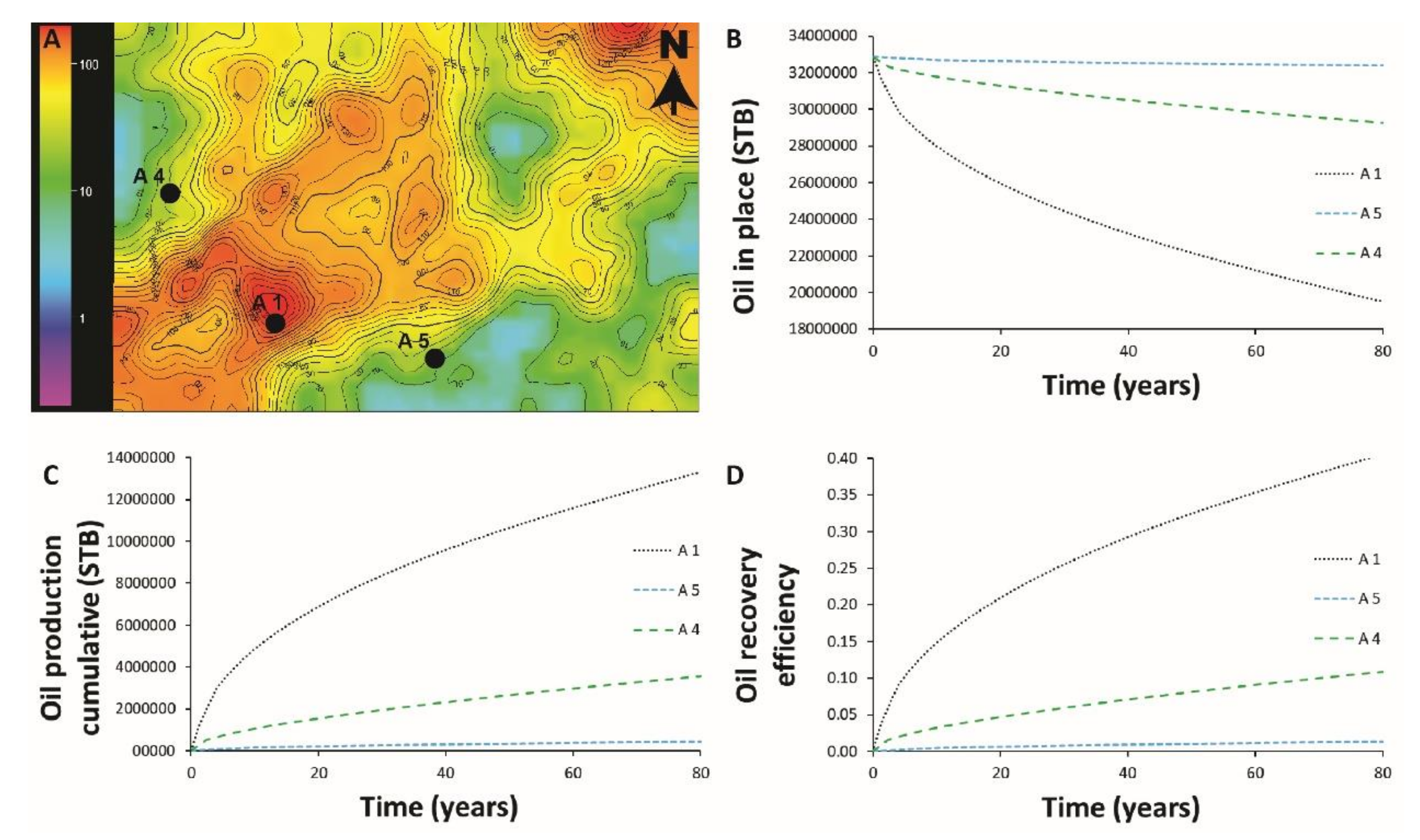
- Wells A 4 and A 5, which represent production from the flanks of the channel, showed markedly lower production indicators, i.e., ORE values of 0.04 and 0.006, respectively; COP values of 1.5 × 10⁶ (STB) and 0.21 × 10⁶ (STB), respectively; and OIP values of 31.2 × 10⁶ and 32.6 × 10⁶, respectively (Figure 15).
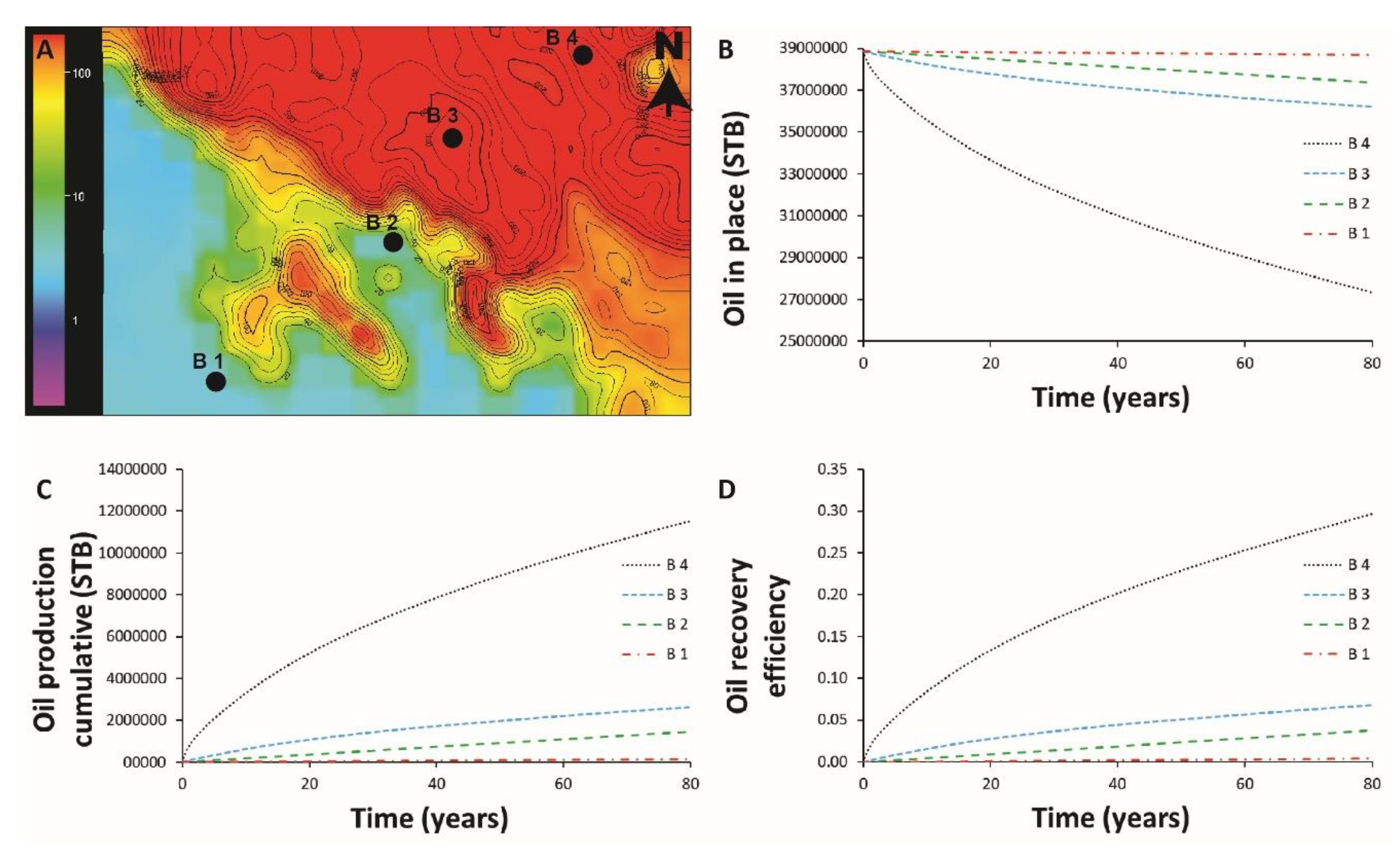
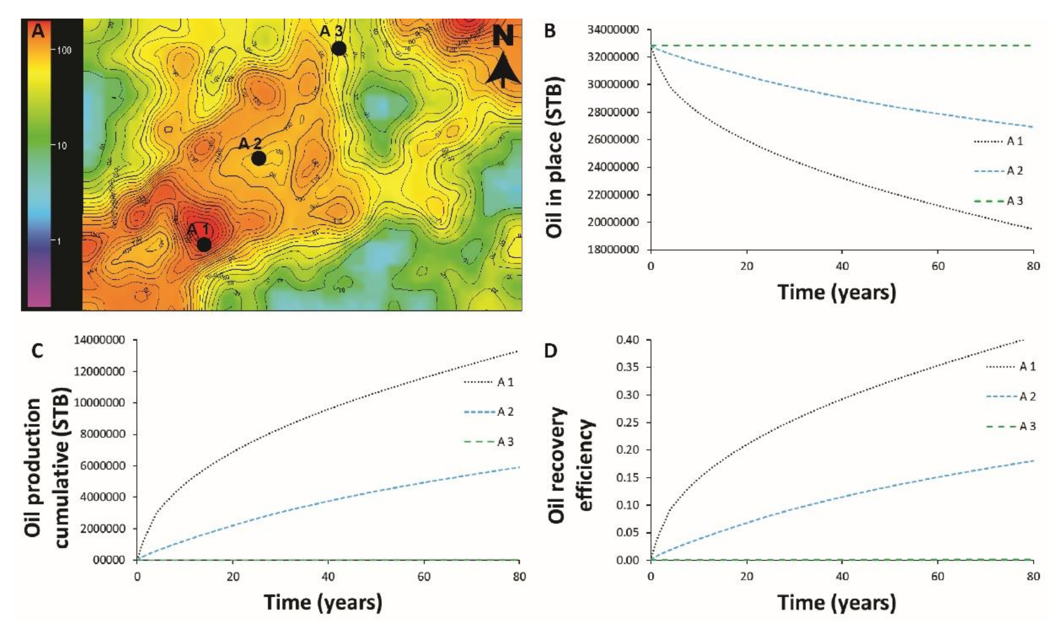
5.5.3. Third Transect
- OIP decreased from updip areas to downdip areas (OIP was 33.6 × 10⁶, 37.7 × 10⁶, 38.4 × 10⁶, and 38.8 × 10⁶ (STB) for Wells B 1–B 4, respectively (Figure 16D)).
6. Discussion
6.1. Similarity of the 3D Model to the Modern Analog and Stratigraphic Record
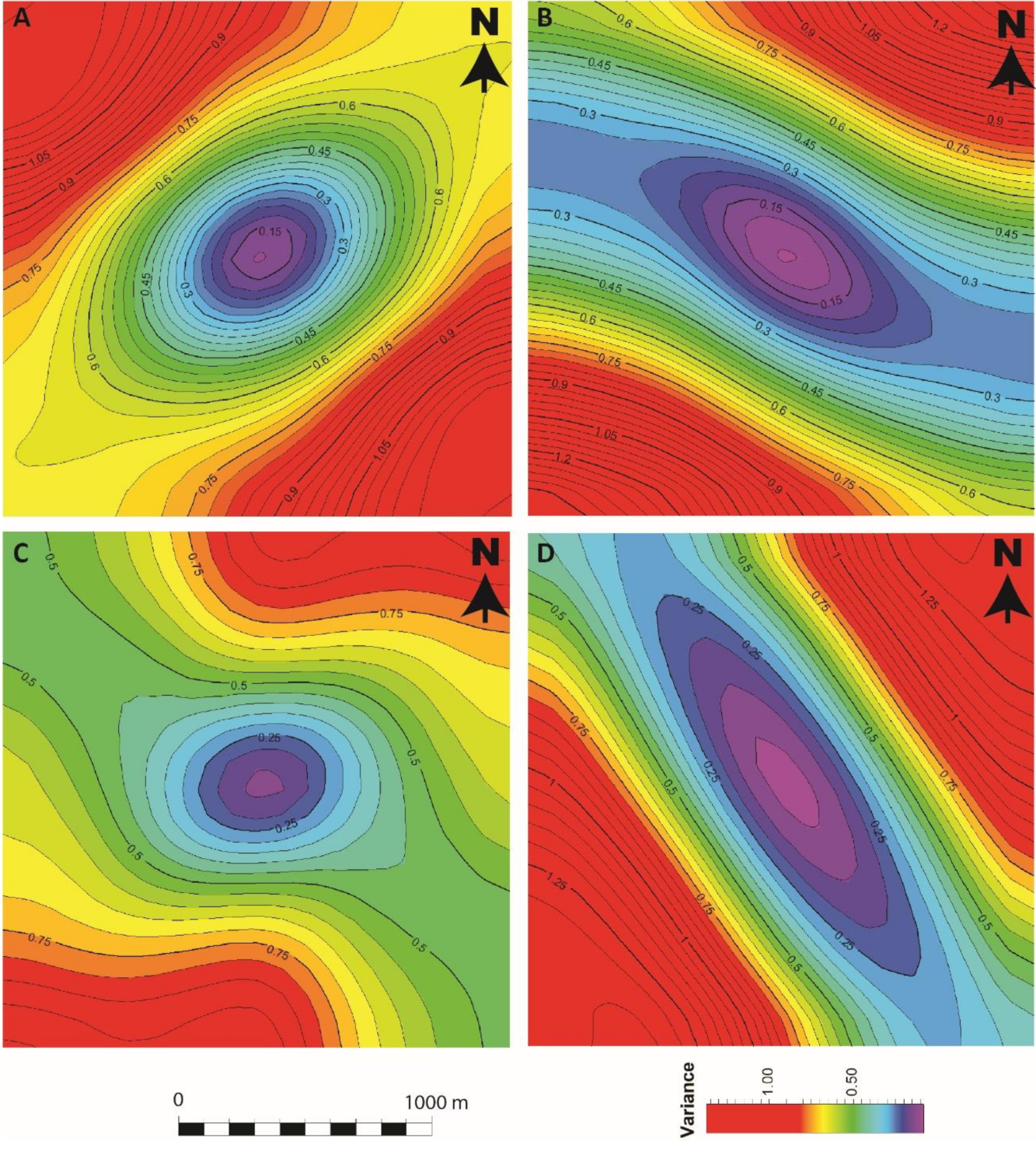
6.2. Understanding Permeability Anisotropy Using Variogram Parameters
6.3. Understanding Permeability Anisotropy with a Sequence Stratigraphic Framework
6.4. Predicting Permeability Anisotropy Using Production Data and Sequence Stratigraphy
6.5. Implications and Limitations
7. Conclusions
- In the 3D models, porosity and permeability vary vertically and laterally with the variation in lithofacies associations, suggesting depositional controls on permeability anisotropy of the studied tidal flat strata.
- Fluid flow simulation results suggest that hydrocarbon production is influenced significantly by permeability anisotropy.
- The 3D models and the results of the fluid flow simulation reveal patterns and trends in permeability anisotropy and hydrocarbon production that could be linked to the sequence stratigraphic framework.
Author Contributions
Funding
Acknowledgments
Conflicts of Interest
References
- Pickup, G.E.; Ringrose, P.S.; Corbett, P.W.M.; Jensen, J.L.; Sorbie, K.S. Geology, geometry and effective flow. Pet. Geosci. 1995, 1, 37–42. [Google Scholar] [CrossRef]
- Zhang, P.; Pickup, G.; Christie, M. A new practical method for upscaling in highly heterogeneous reservoir models. SPE J. 2008, 13, 68–76. [Google Scholar] [CrossRef]
- Branets, L.V.; Ghai, S.S.; Lyons, S.L.; Wu, X.H. Challenges and technologies in reservoir modeling. Commun. Comput. Phys. 2009. [Google Scholar] [CrossRef]
- Shinn, E.; Lloyd, M.; Ginsburg, R. Anatomy of a Modern Carbonate Tidal-flat, Andros Island, Bahamas. SEPM J. Sediment. Res. 1969, 39. [Google Scholar] [CrossRef]
- Grover, G.; Read, J. Fenestral and Associated Vadose Diagenetic Fabrics of Tidal Flat Carbonates, Middle Ordovician New Market Limestone, Southwestern Virginia. SEPM J. Sediment. Res. 1978, 48. [Google Scholar] [CrossRef]
- Shinn, E.A. Tidal flat environment. Carbonate Depos. Environ. 1983, 33, 172–210. [Google Scholar]
- Pratt, B.R.; JAMES, N.P. The St George Group (Lower Ordovician) of western Newfoundland: Tidal flat island model for carbonate sedimentation in shallow epeiric seas. Sedimentology 1986, 33, 313–343. [Google Scholar] [CrossRef]
- Read, J.F.; Grotzinger, J.P.; Bova, J.A.; Koerschner, W.F. Models for generation of carbonate cycles. Geology 1986, 14, 107–110. [Google Scholar] [CrossRef]
- Rankey, E.C. Spatial patterns of sediment accumulation on a holocene carbonate tidal flat, northwest Andros Island, Bahamas. J. Sediment. Res. 2002, 72, 591–601. [Google Scholar] [CrossRef]
- Rankey, E.C.; Morgan, J. Quantified rates of geomorphic change on a modern carbonate tidal flat, Bahamas. Geology 2002, 30, 583–586. [Google Scholar] [CrossRef]
- Meyer, F.O.; Price, R.C.; Al-Ghamdi, I.A.; Al-Goba, I.M.; Al-Raimi, S.M.; Cole, J.C. Sequential stratigraphy of outcropping strata equivalent to Arab-D reservoir, Wadi Nisah, Saudi Arabia. GeoArabia 1996, 1, 435–456. [Google Scholar]
- Amour, F.; Mutti, M.; Christ, N.; Immenhauser, A.; Tomás, S. Outcrop Analogue for a Mixed Siliciclastic-Carbonate Ramp Reservoir: A Multi-Scale Facies Modeling Approach. In Proceedings of the AAPG International Conference and Exhibition, AAPG, Milan, Italy, 23–26 October 2011. [Google Scholar]
- Purkis, S.J.; Vlaswinkel, B. Visualizing lateral anisotropy in modern carbonates. Am. Assoc. Pet. Geol. Bull. 2012, 96, 1665–1685. [Google Scholar] [CrossRef]
- Eltom, H.; Makkawi, M.; Abdullatif, O.; Alramadan, K. High-resolution facies and porosity models of the upper Jurassic Arab-D carbonate reservoir using an outcrop analogue, central Saudi Arabia. Arab. J. Geosci. 2013, 6, 4323–4335. [Google Scholar] [CrossRef]
- Stanley, R.; Al-Ansi, H.; Weber, L.J.; Snow, J. Spatial modeling of Jurassic Arab formation hierarchical carbonate depositional environment tracts as a guide to reservoir connectivity anisotropies: An example from the Dukhan Field, State of Qatar. In Proceedings of the Society of Petroleum Engineers—International Petroleum Technology Conference 2014, IPTC 2014: Unlocking Energy Through Innovation, Technology and Capability, Doha, Qatar, 19–22 January 2014; pp. 1–15. [Google Scholar]
- Rankey, E.C.; Goodner, H.; Doveton, J. Depositional architecture and petrophysical variability of an oolitic tidal sand shoal: Pennsylvanian (Missourian), Kansas, U.S.A. J. Sediment. Res. 2018. [Google Scholar] [CrossRef]
- Verwer, K.; Oscar, M.T.; Kenter, J.A.M.; Della Porta, G. Evolution of a high-relief carbonate platform slope using 3D digital outcrop models: Lower jurassic djebel bou dahar, high atlas, Morocco. J. Sediment. Res. 2009, 79, 416–439. [Google Scholar] [CrossRef]
- Palermo, D.; Aigner, T.; Nardon, S.; Blendinger, W. Three-dimensional facies modeling of carbonate sand bodies: Outcrop analog study in an epicontinental basin (Triassic, southwest Germany). Am. Assoc. Pet. Geol. Bull. 2010, 94, 475–512. [Google Scholar] [CrossRef]
- Petrovic, A.; Aigner, T.; Pontiggia, M. Facies heterogeneities in a ramp carbonate reservoir analogue: A new high-Resolution approach for 3D facies modelling. J. Pet. Geol. 2018, 41, 155–174. [Google Scholar] [CrossRef]
- Steineke, M.; Koch, T. Geological Reconnaissance of the Coastal Plain of Hasa Province, Northeastern Saudi Arabia; Arabian Oil Company: Dhahran, Saudi Arabia, 1935. [Google Scholar]
- Powers, R.; Ramirez, L.; Redmond, C.; Elberg, E. Geology of the Arabian peninsula. Geol. Surv. Prof. Pap. 1966, 560, 1–147. [Google Scholar]
- Iriem, O. Miocene tidal flat stromatolites of the Dam Formation, Sandi Arabia. Arab. J. Sci. Eng. 1987, 12, 145–153. [Google Scholar]
- Alkhaldi, F. Controls on Hierarchy of Miocene Buildups within a High Resolution Cycle Stratigraphic Framework of Dam Formation, Lidam Area, Saudi Arabia. MSc Thesis, King Fahd University of Petroleum and Minerals, Dhahran, Saudi Arabia, 2009. [Google Scholar]
- Ali, S. High-Resolution Stratigraphic Architecture and Sedimentological Heterogeneity within the Miocene Dam Formation, Eastern Province, Eastern Saudi Arabia; King Fahd University of Petroleum and Minerals: Dhahran, Saudi Arabia, 2015. [Google Scholar]
- Bashri, M.; Abdullatif, O.; Salih, M. Sedimentology and facies analysis of Miocene mixed siliciclastic–carbonate deposits of the Dam Formation in Al Lidam area, Eastern Saudi Arabia. Arab. J. Geosci. 2017. [Google Scholar] [CrossRef]
- Abdelkarim, A.A.; Abdullatif, O.M.; Babalola, L.O.; Makkawi, M.H.; Yassin, M.A. High-resolution lithofacies and porosity modeling of the mixed siliciclastic–carbonate deposits of the Burdigalian Dam Formation, Eastern Saudi Arabia. Int. J. Earth Sci. 2019. [Google Scholar] [CrossRef]
- Weijermars, R. Surface geology, lithostratigraphy and Tertiary growth of the Dammam Dome, Saudi Arabia: A new field guide. GeoArabia 1999, 4, 199–226. [Google Scholar]
- Jung, A.; Aigner, T. Carbonate geobodies: Hierarchical classification and database—A new workflow for 3D reservoir modelling. J. Pet. Geol. 2012, 35, 49–65. [Google Scholar] [CrossRef]
- Purkis, S.J.; Rowlands, G.P.; Kerr, J.M. Unravelling the influence of water depth and wave energy on the facies diversity of shelf carbonates. Sedimentology 2015, 62, 541–565. [Google Scholar] [CrossRef]
- Harris, P.M.; Purkis, S.J.; Ellis, J. Analyzing spatial patterns in modern carbonate sand bodies from Great Bahama Bank. J. Sediment. Res. 2011. [Google Scholar] [CrossRef]
- Rankey, E.C.; Enos, P.; Steffen, K.; Druke, D. Lack of impact of Hurricane Michelle on tidal flats, Andros Island, Bahamas: Integrated remote sensing and field observations. J. Sediment. Res. 2004. [Google Scholar] [CrossRef]
- Reeder, S.L.; Rankey, E.C.; Swart, P. A Tale of Two Storms: An Integrated Field, Remote Sensing and Modelling Study Examining the Impact of Hurricanes Frances and Jeanne on Carbonate Systems, Bahamas. In Perspectives in Carbonate Geology; International Association of Sedimentologists; Blackwell Publishing Ltd, 2009; pp. 75–90. [Google Scholar] [CrossRef]
- Harris, A.D.; Covault, J.A.; Madof, A.S.; Tao, S.U.N.; Sylvester, Z.; Granjeon, D. Three-dimensional numerical modeling of eustatic control on continental-margin sand distribution. J. Sediment. Res. 2016, 86, 1434–1443. [Google Scholar] [CrossRef]
- Cantrel, D.L.; Nicholson, P.; Hughes, G.; Miller, M.; Bhullar, A.G.; Abdelbagi, S.T.; Norton, A.K. Tethyan Petroleum Systems of Saudi Arabia. In Memoir 106: Petroleum Systems of the Tethyan Region; 2014. [Google Scholar] [CrossRef]


| Lithofacies Association | Lithofacies | Texture | Grain Types | Sedimentary Structures |
|---|---|---|---|---|
| Mud-dominated tidal flat | Interbedded mudstone and evaporites | Mudstone and evaporites | – | Some lamination |
| Interbedded cross-bedded sandstone and mudstone | Sandstone and mudstone | Quartz grains | Flaser bedding, tidal bundles and reactivation surfaces | |
| Stromatolite | Boundstone | – | Lamination | |
| Grain-dominated tidal channels | Channelized medium sandstone | Sandstone | Quartz and skeletal grains | Herringbone cross-bedding |
| Trough cross-bedded sandstone | Sandstone | Quartz grains | Trough cross-bedding | |
| Interbedded cross-bedded coarse limestone and mudstone | Grainstone and mudstone | Ooids and skeletal grains | Fenestrae vugs and tepee structure | |
| Intraformational limestone conglomerate | Grainstone | Mud clasts | – | |
| Planar cross-bedded skeletal peloidal grainstone | Grainstone | Skeletal and peloidal grains | Planar cross-bedding | |
| Grain-dominated skeletal oolitic shoal | Herringbone cross-bedded skeletal oolitic grainstone | Grainstone | Ooids and skeletal grains | Herringbone cross bedding and keystone vugs |
| Trough cross-bedded aggregate intraclast oolitic grainstones | Grainstone | Aggregate, intraclasts and ooids | Trough cross-bedding | |
| Massive peloidal skeletal packstone | Grainstone | Peloids and skeletal grains | – | |
| Channelised planar cross-bedded skeletal oolitic grainstone | Grainstone | Ooids, skeletons and grapestones | Planar cross-bedding | |
| Dipping planar-bedded skeletal oolitic grainstone | Grainstone | Ooids and skeletal grains | Planar bedding and lamination | |
| Mud-dominated skeletal oolitic shoal fringe | Massive skeletal wackestone | Wackestone | Skeletal grains | – |
| Massive quartz skeletal peloidal wacke-packstone | Wackestone–packstone | Quartz, skeletal and pellets | – |
| Variogram Range (m) | Variogram Direction | Variogram Sill | |||||
|---|---|---|---|---|---|---|---|
| Lithofacies Association | Major | Minor | Vertical | Major | Minor | Major | Minor |
| Mud-dominated tidal flat | 2000 | 1000 | 0.4 | NW-SE | NE-SW | 0.99 | 0.99 |
| Grain-dominated tidal channels | 1200 | 500 | 1 | NE-SW | NW-SE | 0.99 | 0.99 |
| Grain-dominated skeletal oolitic shoal | 2000 | 1000 | 0.4 | NW-SE | NE-SW | 0.99 | 0.99 |
| Mud-dominated skeletal oolitic shoal fringe | 2000 | 1000 | 0.4 | NW-SE | NE-SW | 0.99 | 0.99 |
| Lithofacies proportion (%) | |||||
|---|---|---|---|---|---|
| Lithofacies Association | Entire 3D reservoir | Zone 1 | Zone 2 | Zone 3 | Zone 4 |
| Mud-dominated tidal flat | 38.4 | 42 | 0 | 0 | 0 |
| Grain-dominated tidal channels | 15 | 26.8 | 0 | 18.6 | 0 |
| Grain-dominated skeletal oolitic shoal | 14.3 | 31.2 | 48.2 | 0 | 81.5 |
| Mud-dominated skeletal oolitic shoal fringe | 32.3 | 0 | 51.8 | 81.4 | 18.5 |
Publisher’s Note: MDPI stays neutral with regard to jurisdictional claims in published maps and institutional affiliations. |
© 2020 by the authors. Licensee MDPI, Basel, Switzerland. This article is an open access article distributed under the terms and conditions of the Creative Commons Attribution (CC BY) license (http://creativecommons.org/licenses/by/4.0/).
Share and Cite
Eltom, H.A.; Saraih, N.A.; Esteva, O.G.; Kusuma, L.; Ahmed, S.; Yassin, M.A. Three-Dimensional Modeling and Fluid Flow Simulation for the Quantitative Description of Permeability Anisotropy in Tidal Flat Carbonate. Energies 2020, 13, 5557. https://doi.org/10.3390/en13215557
Eltom HA, Saraih NA, Esteva OG, Kusuma L, Ahmed S, Yassin MA. Three-Dimensional Modeling and Fluid Flow Simulation for the Quantitative Description of Permeability Anisotropy in Tidal Flat Carbonate. Energies. 2020; 13(21):5557. https://doi.org/10.3390/en13215557
Chicago/Turabian StyleEltom, Hassan A., Nabil A. Saraih, Oliver G. Esteva, Lundi Kusuma, Saleh Ahmed, and Mohamed A. Yassin. 2020. "Three-Dimensional Modeling and Fluid Flow Simulation for the Quantitative Description of Permeability Anisotropy in Tidal Flat Carbonate" Energies 13, no. 21: 5557. https://doi.org/10.3390/en13215557
APA StyleEltom, H. A., Saraih, N. A., Esteva, O. G., Kusuma, L., Ahmed, S., & Yassin, M. A. (2020). Three-Dimensional Modeling and Fluid Flow Simulation for the Quantitative Description of Permeability Anisotropy in Tidal Flat Carbonate. Energies, 13(21), 5557. https://doi.org/10.3390/en13215557