Entropy Generation in a Dissipative Nanofluid Flow under the Influence of Magnetic Dissipation and Transpiration


Abstract
1. Introduction
2. Statement of the Problem and Governing Equations
3. Solution Methodology
3.1. Closed-Form Solution of Momentum Balance Equation
3.2. Solution of Energy Balance Equation via Laplace Transform
4. Analysis of Entropy Generation
4.1. Bejan Number
5. Results and Discussion
6. Concluding Remarks
- The decrement in motion is seen for both and nanofluids with increasing and .
- The velocity of the nanofluid is higher than that of the nanofluid.
- The temperature is observed to decrease with increasing values of .
- The temperature increases as , , and increase.
- The thermal boundary layer (TBL) width of the nanoliquid is greater than that of the nanoliquid.
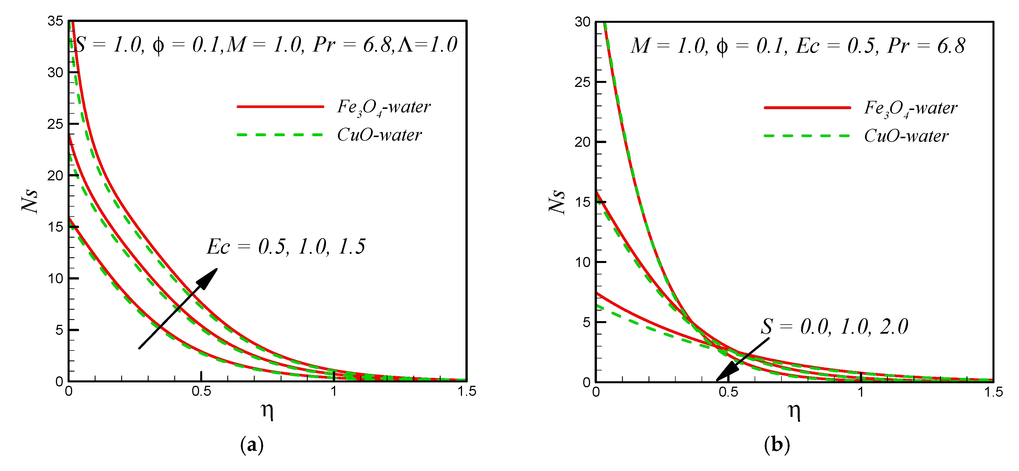
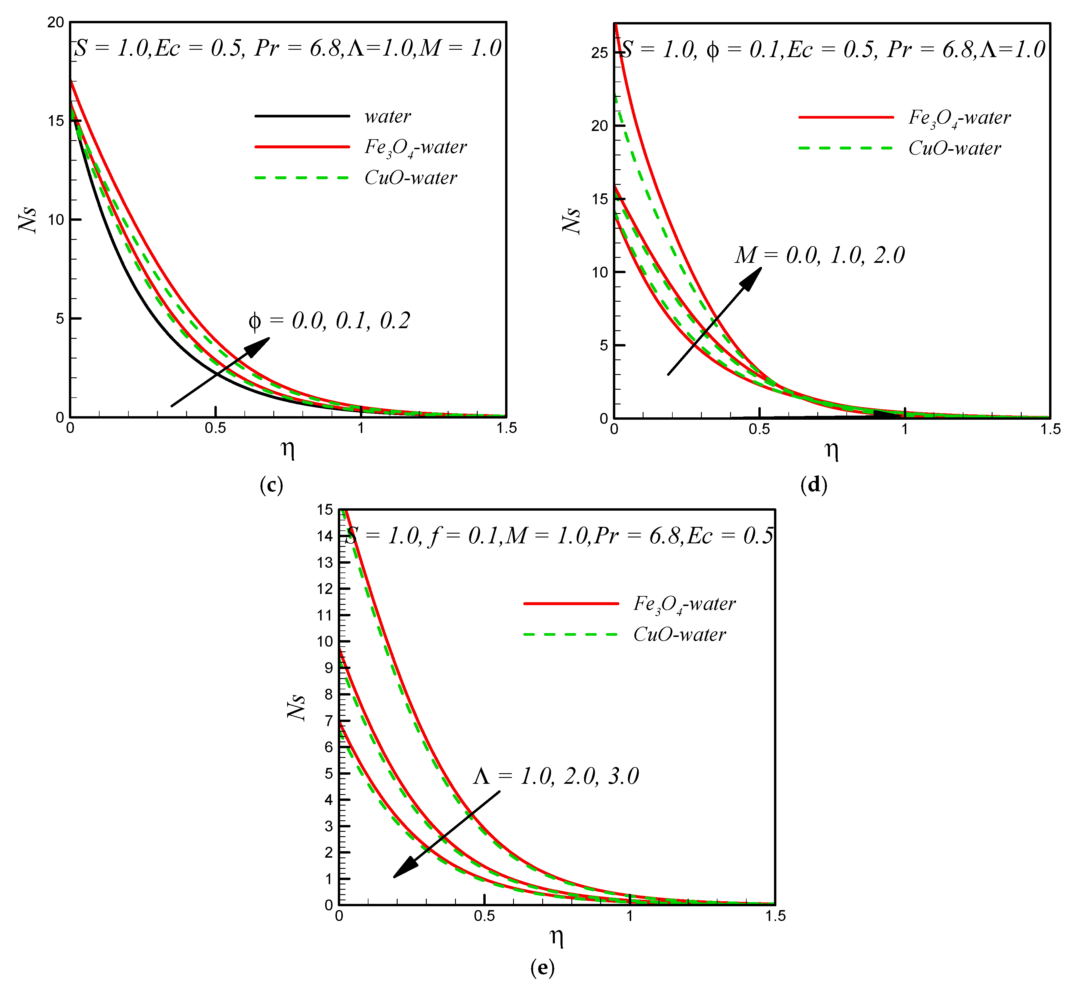
- The entropy generation number is directly related to the Eckert number and solid volume fraction .
- Entropy generation by nonconservative forces is higher in the nanoliquid than in the nanoliquid.
Author Contributions
Funding
Acknowledgments
Conflicts of Interest
Nomenclature
| Dimensional constant | ||
| (Dimensionless) | Bejan number | |
| The applied magnetic field. (“I” shows electric current) | ||
| Specific heat at a constant pressure of a base fluid | ||
| Specific heat at a constant pressure of nanofluid | ||
| (Dimensionless) | Eckert number | |
| (Dimensionless) | Velocity normal to the solid surface | |
| (Dimensionless) | Velocity along the solid surface | |
| Current density | ||
| Thermal conductivity of nanofluid | ||
| Thermal conductivity of the base fluid | ||
| Thermal conductivity of nanoparticle | ||
| (Dimensionless) | Magnetic parameter | |
| (Dimensionless) | Entropy generation due to heat transfer | |
| (Dimensionless) | Entropy generation due to viscous dissipation | |
| (Dimensionless) | Entropy generation due to the magnetic field | |
| (Dimensionless) | Entropy generation number | |
| (Dimensionless) | Prandtl number | |
| (Dimensionless) | Mass transfer parameter | |
| Rate of volumetric entropy generation | ||
| Characteristic entropy generation | ||
| The temperature inside the boundary layer | ||
| The temperature at the solid boundary | ||
| The temperature of fluid outside the thermal boundary layer | ||
| The velocity of a stretching sheet | ||
| Velocity component along the surface of the solid body | ||
| Constant | ||
| Velocity component normal to the surface of the solid body | ||
| Normal velocity component at the boundary | ||
| ) | Cartesian coordinates |
Greek Symbols
| (Dimensionless) | Similarity variable | |
| Dynamic viscosity of a base fluid | ||
| Dynamic viscosity of nanofluid | ||
| Kinematic viscosity of nanofluid | ||
| Nanofluid density | ||
| The density of a base fluid | ||
| Density of nanoparticles | ||
| Electric conductivity | ||
| The electric conductivity of a base fluid | ||
| The electric conductivity of nanoparticle | ||
| (Dimensionless) | Temperature | |
| (Dimensionless) | The solid volume fraction of nanoparticles | |
| (Dimensionless) | Temperature difference parameter |
References
- Wang, C.Y. Exact solutions of the steady-state Navier-Stockes equations. Annu. Rev. Fluid Mech. 1991, 23, 159–177. [Google Scholar] [CrossRef]
- Hui, W.H. Exact solutions of the unsteady two-dimensional Navier-Stokes equations. J. Appl. Math. Phys. 1987, 38, 689–702. [Google Scholar] [CrossRef]
- Polyanin, A.D. Exact solutions to the Navier-Stokes equations with generalized separation of variables. Dokl. Phys. 2001, 46, 726–731. [Google Scholar] [CrossRef]
- Al-Mdallal, Q.M. A new family of exact solutions to the unsteady Navier–Stokes equations using canonical transformation with complex coefficients. Appl. Math. Comput. 2008, 196, 303–308. [Google Scholar] [CrossRef]
- Daly, E.; Basser, H.; Rudman, M. Exact solutions of the Navier-Stokes equations generalized for flow in porous media. Eur. Phys. J. Plus 2018, 133, 173. [Google Scholar] [CrossRef]
- Crane, L.J. Flow past a stretching plate. Zeitschrift für Angewandte Mathematik und Physik 1970, 4, 645–647. [Google Scholar] [CrossRef]
- Fang, T.; Zhang, J.; Yao, S. Slip MHD viscous flow over a stretching sheet—An exact solution. Commun. Nonlinear Sci. Numer. Simul. 2009, 14, 3731–3737. [Google Scholar] [CrossRef]
- Fang, T.; Zhang, J. Closed-form exact solutions of MHD viscous flow over a shrinking sheet. Commun. Nonlinear Sci. Numer. Simul. 2009, 14, 2853–2857. [Google Scholar] [CrossRef]
- Liu, I.-C. Exact Solutions for a Fluid-Saturated Porous Medium with Heat and Mass Transfer. J. Mech. 2011, 21, 57–62. [Google Scholar] [CrossRef]
- Turkyilmazoglu, M. Mixed convection flow of magnetohydrodynamic micropolar fluid due to a porous heated/cooled deformable plate: Exact solutions. Int. J. Heat Mass Transf. 2017, 106, 127–134. [Google Scholar] [CrossRef]
- Khan, Z.H.; Qasim, M.; Ishfaq, N.; Khan, W.A. Dual Solutions of MHD Boundary Layer Flow of a Micropolar Fluid with Weak Concentration over a Stretching/Shrinking Sheet. Commun. Theor. Phys. 2017, 67, 449. [Google Scholar] [CrossRef]
- Bejan, A. A Study of Entropy Generation in Fundamental Convective Heat Transfer. J. Heat Transf. 1979, 101, 718–725. [Google Scholar] [CrossRef]
- Bejan, A. The thermodynamic design of heat and mass transfer processes and devices. Int. J. Heat Fluid Flow 1987, 8, 258–276. [Google Scholar] [CrossRef]
- Butt, A.S.; Ali, A.; Mehmood, A. Entropy analysis in MHD nanofluid flow near a convectively heated stretching surface. Int. J. Exergy 2016, 20, 318–342. [Google Scholar] [CrossRef]
- Das, S.; Chakraborty, S.; Jana, R.N.; Makinde, O.D. Entropy analysis of unsteady magneto-nanofluid flow past accelerating stretching sheet with convective boundary condition. Appl. Math. Mech. 2015, 36, 1593–1610. [Google Scholar] [CrossRef]
- Hakeem, A.K.A.; Govindaraju, M.; Ganga, B.; Kayalvizhi, M. Second law analysis for radiative MHD slip flow of a nanofluid over a stretching sheet with non-uniform heat source effect. Sci. Iran. 2016, 23, 1524–1538. [Google Scholar] [CrossRef]
- Rashidi, M.M.; Freidoonimehr, N. Analysis of Entropy Generation in MHD Stagnation-Point Flow in Porous Media with Heat Transfer. Int. J. Comput. Methods Eng. Sci. Mech. 2014, 15, 345–355. [Google Scholar] [CrossRef]
- Makinde, O.D. Entropy analysis for MHD boundary layer flow and heat transfer over a flat plate with a convective surface boundary condition. Int. J. Exergy 2012, 10, 142. [Google Scholar] [CrossRef]
- Butt, A.S.; Ali, A.; Mehmood, A. Numerical investigation of magnetic field effects on entropy generation in viscous flow over a stretching cylinder embedded in a porous medium. Energy 2016, 99, 237–249. [Google Scholar] [CrossRef]
- Ding, H.; Li, Y.; Lakzian, E.; Wen, C.; Wang, C. Entropy generation and exergy destruction in condensing steam flow through turbine blade with surface roughness. Energy Convers. Manag. 2019, 196, 1089–1104. [Google Scholar] [CrossRef]
- Al-Odat, M.Q.; Damseh, R.A.; Al-Nimr, M.A. Effect of Magnetic Field on Entropy Generation Due to Laminar Forced Convection Past a Horizontal Flat Plate. Entropy 2004, 4, 293–303. [Google Scholar] [CrossRef]
- Rashidi, M.M.; Mohammadi, F.; Abbasbandy, S.; Alhuthali, M.S. Entropy Generation Analysis for Stagnation Point Flow in a Porous Medium over a Permeable Stretching Surface. J. Appl. Fluid Mech. 2015, 8, 753–765. [Google Scholar] [CrossRef]
- Das, S.; Jana, R.N.; Makinde, O.D. Entropy generation in hydromagnetic and thermal boundary layer flow due to radial stretching sheet with Newtonian heating. J. Heat Mass Transf. Res. 2015, 2, 51–61. [Google Scholar]
- Ajibade, A.O.; Jha, B.K.; Omame, A. Entropy generation under the effect of suction/injection. Appl. Math. Model. 2011, 35, 4630–4646. [Google Scholar] [CrossRef]
- Govindaraju, M.; Ganga, B.; Hakeem, A.K.A. Second law analysis on radiative slip flow of nanofluid over a stretching sheet in the presence of lorentz force and heat generation/absorption. Front. Heat Mass Transf. 2017, 8, 1–8. [Google Scholar] [CrossRef]
- Milanese, M.; Iacobazzi, F.; Colangelo, G.; Risi, A. An investigation of layering phenomenon at the liquid–solid interface in Cu and CuO based nanofluids. Int. J. Heat Mass Transf. 2016, 103, 564–571. [Google Scholar] [CrossRef]
- Iacobazzi, F.; Milanese, M.; Colangelo, G.; Lomascolo, M.; Risi, A. An explanation of the Al2O3 nanofluid thermal conductivity based on the phonon theory of liquid. Energy 2016, 116, 786–794. [Google Scholar] [CrossRef]
- Colangelo, G.; Milanese, M.; De Risi, A. Numerical simulation of thermal efficiency of an innovative Al2O3 nanofluid solar thermal collector: Influence of nanoparticles concentration. Therm. Sci. 2017, 21, 2769–2779. [Google Scholar] [CrossRef]
- Colangelo, G.; Favale, E.; Milanese, M.; de Risi, A.; Laforgia, D. Cooling of electronic devices: Nanofluids contribution. Appl. Therm. Eng. 2017, 127, 421–435. [Google Scholar] [CrossRef]
- Colangelo, G.; Favale, E.; Miglietta, P.; Milanese, M.; de Risi, M. Thermal conductivity, viscosity and stability of Al2O3-diathermic oil nanofluids for solar energy systems. Energy 2016, 95, 124–136. [Google Scholar] [CrossRef]
- Colangelo, G.; Favale, E.; Milanese, M.; Starace, G.; De Risi, A. Experimental Measurements of Al2O3 and CuO Nanofluids Interaction with Microwaves. J. Energy Eng. 2017, 143, 04016045. [Google Scholar] [CrossRef]
- Iacobazzi, F.; Milanese, M.; Colangelo, G.; de Risi, A. A critical analysis of clustering phenomenon in Al2O3 nanofluids. J. Therm. Anal. Calorim. 2018, 135, 371–377. [Google Scholar] [CrossRef]
- Hsiao, K.-L. Stagnation electrical MHD nanofluid mixed convection with slip boundary on a stretching sheet. Appl. Therm. Eng. 2016, 98, 850–861. [Google Scholar] [CrossRef]
- Ma, Y.; Mohebbi, R.; Rashidi, M.; Yang, Z.; Sheremet, M. Nanoliquid thermal convection in I-shaped multiple-pipe heat exchanger under magnetic field influence. Phys. A Stat. Mech. Its Appl. 2020, 550, 124028. [Google Scholar] [CrossRef]
- Wakif, A.; Chamkha, A.; Thumma, T.; Animasaun, I.L.; Sehaqui, R. Thermal radiation and surface roughness effects on the thermo-magneto-hydrodynamic stability of alumina–copper oxide hybrid nanofluids utilizing the generalized Buongiorno’s nanofluid model. J. Therm. Anal. Calorim. 2020, 1–20. [Google Scholar] [CrossRef]
- Hsiao, K.-L. Nanofluid flow with multimedia physical features for conjugate mixed convection and radiation. Comput. Fluids 2014, 104, 1–8. [Google Scholar] [CrossRef]
- Ma, Y.; Mohebbi, R.; Rashidi, M.M.; Yang, Z. MHD convective heat transfer of Ag-MgO/water hybrid nanofluid in a channel with active heaters and coolers. Int. J. Heat Mass Transf. 2019, 137, 714–726. [Google Scholar] [CrossRef]
- Prasad, K.V.; Vaidya, H.; Makinde, O.D.; Vajravelu, K.; Wakif, A.; Basha, H. Comprehensive examination of the three-dimensional rotating flow of a UCM nanoliquid over an exponentially stretchable convective surface utilizing the optimal homotopy analysis method. Front. Heat Mass Transf. 2020, 14. [Google Scholar] [CrossRef]
- Gebhart, B. Effects of viscous dissipation in natural convection. J. Fluid Mech. 1962, 14, 225–232. [Google Scholar] [CrossRef]
- Desale, S.; Pradhan, V.H. Numerical Solution of Boundary Layer Flow Equation with Viscous Dissipation Effect Along a Flat Plate with Variable Temperature. Procedia Eng. 2015, 127, 846–853. [Google Scholar] [CrossRef]
- Vajravelu, K.; Hadjinicolaou, A. Heat transfer in a viscous fluid over a stretching sheet with viscous dissipation and internal heat generation. Int. Commun. Heat Mass Transf. 1993, 20, 417–430. [Google Scholar] [CrossRef]
- Alsabery, A.; Saleh, H.; Hashim, I. Effects of Viscous Dissipation and Radiation on MHD Natural Convection in Oblique Porous Cavity with Constant Heat Flux. Adv. Appl. Math. Mech. 2017, 9, 463–484. [Google Scholar] [CrossRef]
- Mohamed, M.K.A.; Sarif, N.M.; Noar, N.A.Z.M.; Salleh, M.Z.; Ishak, A. Viscous dissipation effect on the mixed convection boundary layer flow towards solid sphere. Trans. Sci. Technol. 2016, 3, 59–67. [Google Scholar]
- Jamaludin, A.; Nazar, R.; Khan, I. AIP Conference Proceedings; Boundary Layer Flow and Heat Transfer in a Viscous Fluid over a Stretching Sheet with Viscous Dissipation, Internal Heat Generation and Prescribed Heat Flux; AIP Publishing LLC: New York, NY, USA, 2017; Volume 1870, p. 040029. [Google Scholar] [CrossRef]
- Makinde, O.D. Effects of viscous dissipation and Newtonian heating on boundary-layer flow of nanofluids over a flat plate. Int. J. Numer. Methods Heat Fluid Flow 2013, 23, 1291–1303. [Google Scholar] [CrossRef]
- Motsumi, T.G.; Makinde, O.D. Effects of thermal radiation and viscous dissipation on boundary layer flow of nanofluids over a permeable moving flat plate. Phys. Scr. 2012, 86, 1–8. [Google Scholar] [CrossRef]
- Minkowycz, W.J.; Sparrow, E.M.; Abraham, J.P. Nanoparticle Heat Transfer and Fluid Flow; CRC Press: Boca Raton, FL, USA, 2012. [Google Scholar]
- Bianco, V.; Manca, O.; Nardini, S.; Vafai, K. Heat Transfer Enhancement of Nanofluids; CRC Press: Boca Raton, FL, USA, 2015. [Google Scholar]
- Kleinstreuer, C.; Feng, Y. Experimental and Theoretical Studies of Nanofluid Thermal Conductivity Enhancement: A Review. Nanoscale Res. Lett. 2011, 6, 229. [Google Scholar] [CrossRef]
- Bashirnezhad, K.; Bazri, S.; Safaei, M.R.; Goodarzi, M.; Dahari, M.; Mahian, O.; Dalkılıça, A.S.; Wongwises, S. Viscosity of nanofluids: A review of recent experimental studies. Int Commun Heat Mass Transf. 2016, 73, 114–123. [Google Scholar] [CrossRef]
- Sheikholeslami, M. Nanofluid Heat and Mass Transfer in Engineering Problems; Intech Open: Rijeka, Croatia, 2017. [Google Scholar]
- Sajid, M.U.; Ali, H.M. Recent advances in application of nanofluids in heat transfer devices: A critical review. Renew. Sustain. Energy Rev. 2019, 103, 556–592. [Google Scholar] [CrossRef]


| Thermophysical Property of Nanofluid | Symbol | Defined |
|---|---|---|
| Thermal conductivity | here, represents sold volume fraction of nanoparticles. | |
| Viscosity | ||
| Electric conductivity | ||
| Heat capacitance | ||
| Density |
| Physical Properties | |||
|---|---|---|---|
| 4179 | 531.8 | 670 | |
| (W/mK | 0.613 | 76.5 | 6.0 |
| 997.1 | 6320 | 5200 | |
| 5180 | 2.7 × 10⁻⁸ | 25,000 | |
| Pr (-) | 6.8 | - | - |
Publisher’s Note: MDPI stays neutral with regard to jurisdictional claims in published maps and institutional affiliations. |
© 2020 by the authors. Licensee MDPI, Basel, Switzerland. This article is an open access article distributed under the terms and conditions of the Creative Commons Attribution (CC BY) license (http://creativecommons.org/licenses/by/4.0/).
Share and Cite
Lu, D.; Afridi, M.I.; Allauddin, U.; Farooq, U.; Qasim, M. Entropy Generation in a Dissipative Nanofluid Flow under the Influence of Magnetic Dissipation and Transpiration. Energies 2020, 13, 5506. https://doi.org/10.3390/en13205506
Lu D, Afridi MI, Allauddin U, Farooq U, Qasim M. Entropy Generation in a Dissipative Nanofluid Flow under the Influence of Magnetic Dissipation and Transpiration. Energies. 2020; 13(20):5506. https://doi.org/10.3390/en13205506
Chicago/Turabian StyleLu, Dianchen, Muhammad Idrees Afridi, Usman Allauddin, Umer Farooq, and Muhammad Qasim. 2020. "Entropy Generation in a Dissipative Nanofluid Flow under the Influence of Magnetic Dissipation and Transpiration" Energies 13, no. 20: 5506. https://doi.org/10.3390/en13205506
APA StyleLu, D., Afridi, M. I., Allauddin, U., Farooq, U., & Qasim, M. (2020). Entropy Generation in a Dissipative Nanofluid Flow under the Influence of Magnetic Dissipation and Transpiration. Energies, 13(20), 5506. https://doi.org/10.3390/en13205506