Neural Methods Comparison for Prediction of Heating Energy Based on Few Hundreds Enhanced Buildings in Four Season’s Climate

Abstract

Sustainable development and the increasing demand for equitable energy use as well as the reduction of waste of energy are the author’s social and scientific motivations. This new paradigm is the selection of a pertinent methodology to evaluate the efficiency of habitat thermomodernization, which is one of the scientific tasks of the presented study. In order to meet the social and scientific requirements, 380 buildings from the end of the last century (made of large plate technology), which were thermally improved at the beginning of the XXI century, were designed for a comparative analysis of the predictive modelling of heating energy consumption. A specific set of important variables characterizing the examined buildings has been identified. Groups of variables were used to estimate the energy consumption in such a way as to achieve a compromise between the difficulty of obtaining them and the quality of forecast. To predict energy consumption, the six most appropriate neural methods were used: artificial neural networks (ANN), general regression trees (CART), exhaustive regression trees (CHAID), support regression trees (SRT), support vectors (SV), and method multivariant adaptive regression splines (MARS). The quality assessment of the developed models used the mean absolute percentage error (MAPE) also known as mean absolute percentage deviation (MAPD), as well as mean bias error (MBE), coefficient of variance of the root mean square error (CV RMSE) and coefficient of determination (R²), which are accepted as statistical calibration standards by (American Society of Heating, Refrigerating and Air-Conditioning Engineers) ASHRAE. On this basis, the most effective method has been chosen, which gives the best results and therefore allows to forecast with great precision the energy consumption (after thermal improvement) for this type of residential building.

1. Introduction

1.1. Scientific Context and Recent Trends in through Data-Driven Modeling

Tomorrow, and in some cases today, our everyday life will operate within more and more structured smart cyber-physical systems monitoring the physical processes of (personal interests and mobility, commercial and financial activity, electrical energy and water consumption, transport traffic, telecommunication, connected objects, etc.) in our environment, highly contributing to centralized decisions [1]. Deliberately, this study is devoted to only one aspect of energy consumption, limited to the selection of the most efficient methodology to predict the energy consumption of a human habitat in a four-season climate according to Köppen–Geiger climate classification. Dfb is designing warm-summer humid continental climate covering the largest part of Europe and part of the USA and Canada. In contrast to the modern perception of energy, “ἐνέργεια—energeia” was in ancient Greece a qualitative philosophical concept, broad enough to include ideas such as happiness, comfort, and pleasure. Today, energy has become a central problem for each of us, particularly in terms of personal serenity, mainly if financial and/or authorities restrictions play a main role. From one side, quasi monopolistic positioning of energy generation and/or distribution becomes problematic from a social point of view for humans, and on another side, its equitable selection and distribution, as well as general saving become vital [1].

Therefore, the influence and manipulation of decision-makers offer new fields for artificial intelligence (AI) expansion. The development, proliferation, and use of different algorithms for predictive model selection and their validation is one of its important aspects. Big data collection and their treatment are consequently fundamental terms of in system influences [2].

There is no place here to polemicize on the data rich and information poor (DRIP) dilemma. That concept (DRIP) was first used in the 1983 to describe organizations rich in data, but lacking the processes to produce meaningful information and create a competitive advantage. DRIP was since defeated in the private sector with the wise implementation of information technology. That is a part of the Industry 4.0 (shortened to simply I4.) scheme referred to as the fourth industrial revolution. That name is given to the current trend of cognitive computation comprising AI. Many tools are used in AI, including different versions of mathematical optimization based on statistics, rough set methods, artificial neural networks, and economics [3,4]. The AI cognitive aspects draw upon information engineering, including monitoring and computer sciences, as well as philosophy, linguistics, and psychology and many other fields of cognition sciences. Growing digitization contributes to a rising social gap of knowledge also in developed countries due to the positioning of “decision-makers” in “complex situations”. Increasing demands for equitable energy use and the reduction of waste of energy is one of author’s scientific motivations.

1.2. Habitat Thermal Comfort Versus Cognitive and Emotional Dissonance

Human comfort is a feeling of well-being that has a triple origin (physical, functional, and psychic). One of the fundamental characteristics of the human habitat besides location and architecture, is the comfort and particularly in four-season countries, particularly thermal aspects of it.

The most commonly used definition for thermal comfort according to the American Society of Heating, Refrigerating, and Air-Conditioning Engineers (ASHRAE) [5] is “that condition of mind which expresses satisfaction with the thermal environment and is assessed by subjective evaluation”. Immediately the cost of it comes to our mind event if that aspect is omitted. Although thermal sensitivity varies from one person to another, according style of life, to age (the very young and very old being particularly sensitive), gender, dress, education, activity, cultural habits, etc., the basic principles behind thermal comfort are largely universal.

The recent trends in prediction due to credulous and naïve thermomodernization audit should be very carefully analyzed. Such forecasts often do not take into account information about the use of buildings, which leads to discrepancies between theoretical and actual energy consumption.

Moreover, material scientists, architects, and civil engineers are very preoccupied by the methodology of energy consumption evaluation of buildings to be fashioned as well as the improvement of heritage constructions.

Thermal comfort is linked on the one hand to the quality of the thermal insulation and the thermal inertia of the housing, and on the other hand, to the ambient humidity level (hygro-thermal comfort) depending on climate conditions. There is no direct link between thermal comfort and energy bill that varies according to the climatic context and according to the quality of the building.

From the 1960s to the 1980s, the technology of large panels (prefabricated) was very popular in Polish housing construction. The period of the greatest development of housing construction, based on large plate technology, falls in the 1970s. It was a period of planning and the construction of new, large housing estates. It was on them that prefabricated blocks of flats were erected. The assembly of prefabricated buildings on construction sites took place at a fairly fast pace. A characteristic problem for the construction of this period, which was particularly noticeable in the production of prefabricated elements, was the low quality of workmanship. A large percentage of sub-standard, defective elements often hindered and disorganized work on building assembly. Despite many improvements made at the place where the panels were joined, their joints were still difficult to seal. After a short period of use of residential buildings, physical defects could be observed, such as freezing and ventilation of vertical and horizontal joints of prefabricated large panels. This resulted in the formation of moisture and fungus. Sealing with impregnated hemp ropes did not meet the thermal requirements. In addition, the wall thermal insulation standards in force at that time were more than three times lower than those required today. These buildings were characterized by very high energy consumption.

The authors’ interest in this type of building results from the fact that there are about 3.5 million of them in Poland accomodating about 12 million people.

Poland is currently experiencing a big turnaround in regard to national housing policy, with the introduction of specific programs (e.g., Home Plus & Habitat for Humanity) as well as the revision of the thermomodernization policy being an important part of the process. The framework of thermo-modernization in Poland covers the thermal refurbishment of all types of residential and municipal buildings (including schools and hospitals); the local district heating network and local sources of heating; and the installation of renewable energy sources or high efficiency energy equipment. That is the fundament reason for fantastic space selection for scientific studies of different methods.

The new paradigm is the selection of pertinent methodology to evaluate the efficiency of habitat thermomodernization what is one of the tasks of presented study (Figure 1). To satisfy social as well as scientific requirements, the 380 buildings (buildings made of prefabricates) from the end of the last century thermally improved at the beginning of 21st century were selected.

2. Critical Bibliographical Analysis of Estimation Methods for Building’s Energy Demand

The aim here is comparing the estimation methods of energy demand, their capabilities, strengths, and weakness in analyzed examples.

There are numerous methods for forecasting current and future energy needs of buildings which may be divided into engineering, statistical methods, and those based on the artificial intelligence (and also hybrid methods which combine the specified models) [3,4,6,7]. Engineering methods allow to make accurate forecasts of energy demand in a building, but they require a lot of work to carry out the thermal balance of the building. This analysis takes into account the actual operating parameters of individual systems: heating, cooling, and hot water preparation. Such a set of data characterizing the energy needs of buildings allows to determine the energy characteristics of individual buildings and to develop energy demand forecasts for them to ensure thermal comfort (user comfort). Due to the period of time that the balance sheet concerns, these methods can be divided into dynamic and static. Dynamic methods are mainly based on the measurement methodology presented in EN 16798 [8]. This refers to the values characterizing the thermal comfort of a building in particular seasons of the year. The methods from this group are mainly used for thermal calculations in new energy-saving and passive buildings [9,10,11]. They allow to perform a thermal balance of the building in short intervals of time, e.g., hours. They also provide the possibility of very accurate analyses of the building’s thermal balance, taking into account thermal phenomena connected with energy accumulation of building’s structural elements.

The second group of methods, i.e., static models, are based on the EN 13790 [12] standard supplemented by the EN 12831 [13] standard. Contrary to dynamic methods, analyzes of the heat balance are performed over long computational periods, most often covering the entire heating season. Examples of such analyzes are presented, among others in studies [14,15,16].

Statistical methods are usually regression models that are built on the basis of historical results. Regression models are used to forecast energy consumption based on such data as, for example: geometric dimensions, shape coefficient, area of partitions through which heat losses occur, thermal resistance of partitions, air temperature inside and outside the building and the period in which the building was built. Model calculations are performed both at the level of a single building as well as for entire building systems—groups of buildings and even entire cities. In some simplified models, regression is used to find the relationship between the final energy demand and climatic data, e.g., degrees-day of heating season in order to obtain the energy performance index [3,17,18,19,20,21,22,23,24,25,26,27,28]. Artificial neural networks are most often used in artificial intelligence-based forecasting models. These types of model are based on solving non-linear problems, where they are reliably suitable for estimating energy efficiency in various types of buildings. With the use of artificial neural networks, energy consumption was estimated for such processes as, for example: heating and cooling, thermal resistance of partitions, optimization of energy consumption and evaluation of operational parameters, as well as electricity consumption. The use of artificial neural networks for forecasting energy consumption can be found in the works of many authors [3,29,30,31,32,33,34]. These models are built for various types of buildings, where they estimate energy consumption with high precision [3,34].

Most of the presented calculation methods are effective in determining the energy efficiency of buildings. However, there is a need for further research to check the suitability of forecasting methods that could be applied to real buildings with different availability and accuracy of data describing the object from the thermal and operational point of view. Forecasting models focus mainly on estimating energy consumption in existing or simulated facilities, those newly built, and energy-saving (passive) buildings [9,28], where it is possible to obtain reliable data on the insulation of building partitions, ventilation air streams, and the number of their inhabitants [7,9].

However, few works concern residential buildings, in particular, there are no studies on actual residential buildings made of large plate technology (prefabricated), for which it is difficult to obtain detailed and reliable data. In buildings of this type, a frequent problem in thermal calculations is the lack of complete architectural and construction documentation. Moreover, there are other factors that affect the accuracy of calculations, which are caused by, e.g., moisture, aging of the material, the size of ventilation air flow, etc. Therefore, the aim of the research was to determine the usefulness of models based on artificial neural networks for estimating thermal energy consumption in multi-family residential buildings made of prefabricated (made of large panels), which have been thermally improved. Due to different availability and accuracy of data describing the building, different configurations of input variables will be applied and tested during model construction in order to achieve a compromise between the auditor’s efforts to obtain them and the quality of the forecast.

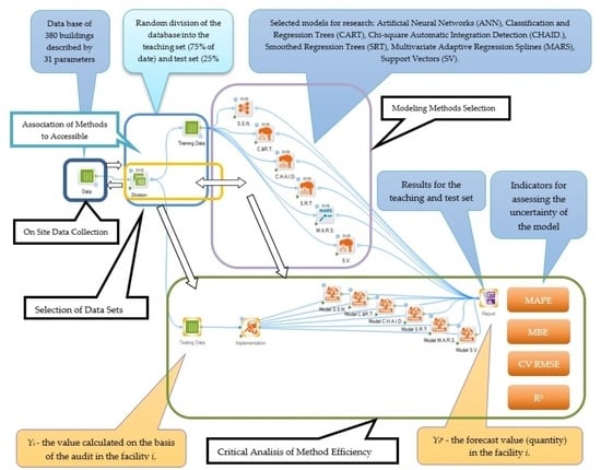
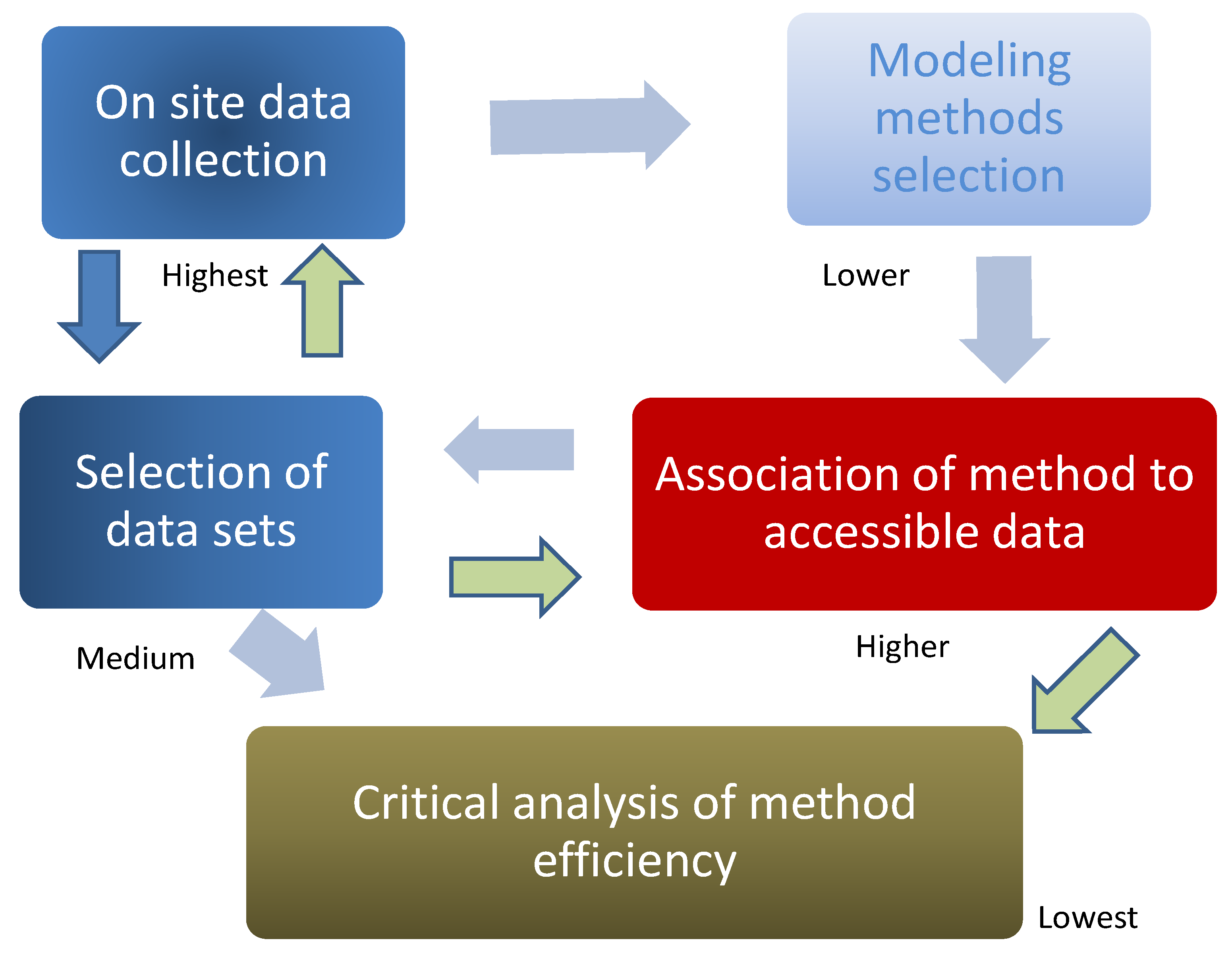
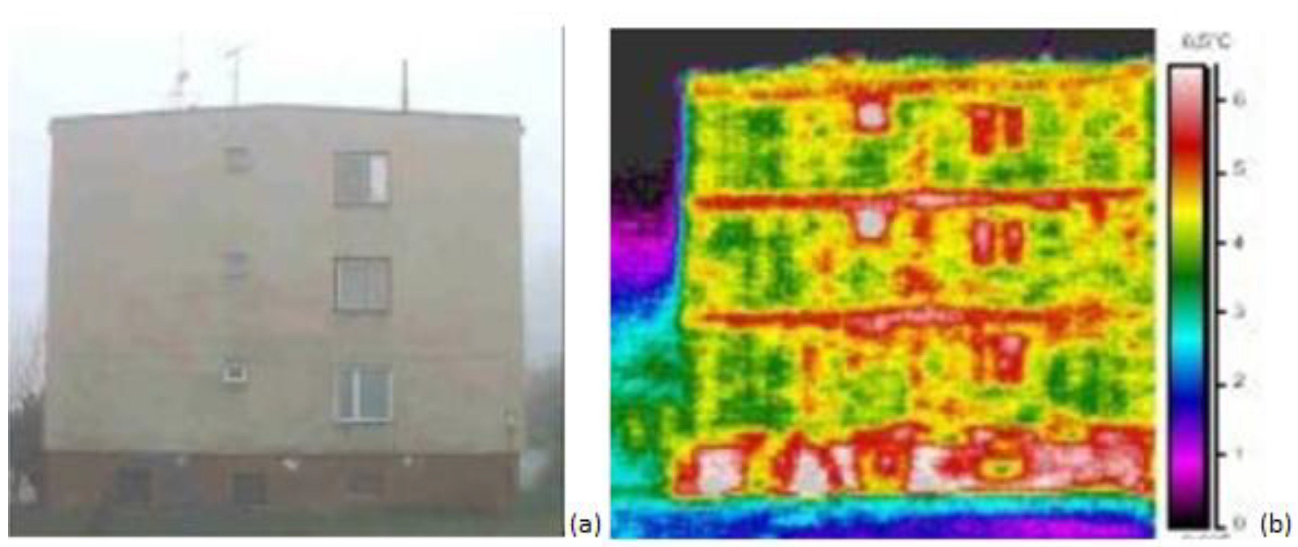
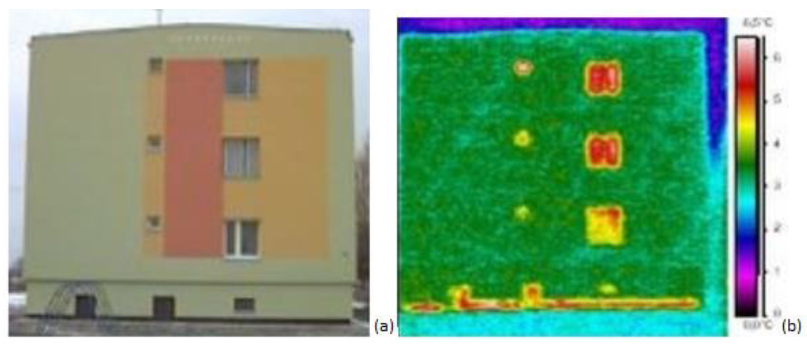
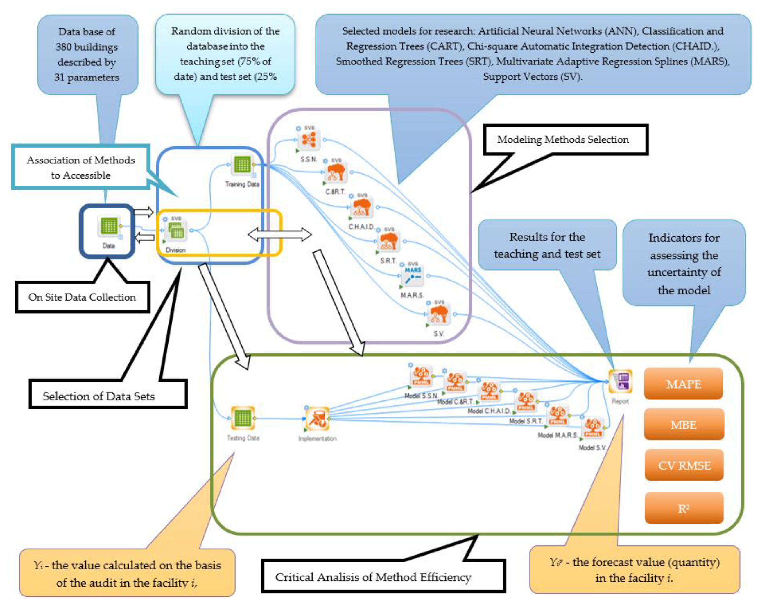
3. Proposed Methodology of Investigations—Experimental Sites and Structure Model

Modelling of the impact of thermal efficiency improvement that works on the heat demand in residential buildings is a very difficult problem mainly due to the fact that it is influenced by a great number of factors. Very generally, they can be divided into factors non ’epistemologically “named” and related to:

• the “construction technology”,
• the “geometry” of the building”,
• the “meteorological” environmental conditions, and
• the “preferences” of their inhabitants.

At each stage of conducting audit calculations, there is a probability of inaccurate estimation of some of the volumes, most often it concerns the physical parameters of buildings and the method of use of the object, which results from the difficulty of collecting all numerical values of the object and its surroundings at a sufficiently high level of precision. This applies in particular to the value of the heat transfer coefficient U of the building shell. The heat transfer coefficient is seemingly an example of a well-defined parameter. The measurement and computational methods for estimating these values are known and quite accurately described. Unfortunately, however, in addition to a few simple cases, proper determination of this value requires a considerable amount of time, in the case of measurement methods, or the use of computer programs, if you want to use computational methods. A frequent problem in auditing activities is the lack of complete architectural and construction documentation of the analyzed objects. In this case, the auditor carries out partitions tests and then calculates the U heat transfer coefficient. Even a correct calculation of the U coefficient may be burdened with an error, because it is necessary to accurately determine the thermal conductivity and thickness of individual layers, which is not always possible, especially in real buildings. Therefore, auditors often use information contained in industry regulations. This approach is the most correct, but in the case of existing buildings it can sometimes lead to a significant error, with the poor condition of the partition, e.g., due to its moisture, aging of the material, etc., results in a higher than normative penetration rate. In many cases, the partition structure is incompatible with the standard requirements, which usually reveals a higher than estimated value of the U-factor. On account of the complexity of this problem, attempts were made to verify the usefulness of the alternative regression method for modelling of the percentage reduction of the annual energy demand in apartment buildings subjected to the improvement of thermal efficiency. From among many available methods of work, this paper investigates effectiveness of the following models: artificial neural networks (ANN), general regression trees (CART), exhaustive regression trees (CHAID), support regression trees (SRT), support vectors (SV), and method multivariant adaptive regression splines (MARS).

The first of the investigated methods were artificial neural network models which originate in the research carried out in the field of artificial intelligence. Research studies on the structure of the models of basic structures occurring in a brain had significant meaning for their development. These papers aimed mainly at the following characteristic features for biological nervous systems which will enable their practical use in technical issues.

The ANN module available in Statistica 13 program was used for construction of the model. When searching for an optimal structure of the network, the number of neurons in the hidden layer was changed from 3 to 15. In the structure of the network, linear, logistic, tangential, exponential, and sinusoidal functions were used as a function activating the transitional and output layer. Calculations were repeated for three teaching network algorithms, i.e., the fastest decrease method, the Broydena–Fletchera–Goldfarba–Shanno (BFGS) algorithm, and the conjugate gradient algorithm.

The second group covered the regression trees models (CART, CHAID), boosted regression trees (SRT) and support vectors (SV). They generate tress where each node (except for leaves) includes the condition for a division and their aim is optimal prediction of the quantity dependent variable. A classic algorithm of CART method was popularized by Breiman [30,35]. On the other hand, (CHAID) algorithm is one of the oldest methods of trees suggested by Kassa [36]. Multivariant adaptive regression splines (MARS) is an implementation of generalization of the technique introduced to common use by Friedman [37,38].

4. Description of Research Methodology and Application

Before the implementation of the main goal of the work, analyzes were carried out to establish a potential list of explanatory variables. During the research, a very extensive database was created, covering 380 buildings made of prefabricated panels for which energy audits were carried out. In particular, the energy consumption in the existing state before thermal modernization was calculated (Figure 2).

For individual buildings the optimum thickness of the insulation layer of individual partitions has been assumed due to the shortest time of return on investment (Figure 3).

The analyzed buildings are heated from the municipal heating network. Therefore, information was collected (based on thermal energy bills) on the actual consumption of heat for heating during the heating season (before and after thermal improvement). To exclude seasonal fluctuations, the actual energy consumption values have been converted (adjusted) to standard season conditions.

The analyzed buildings were described with many parameters. For experimental reasons, most relevant characteristics have been selected. In the first step these sizes were eliminated which were not statistically significantly correlated with the explained size or had a variability coefficient with the value below 10% or were very strongly correlated with each other. The strength of the correlation between the variables was assessed in the Statistica programme. The r-Pearson correlation coefficient would be statistically significant for the significance level p = 0.05. These requirements were met by 31 variables. These variables will be further divided into sets, which were used to check the usefulness of selected models for forecasting.

For the purpose of the work, analyzes were carried out to select the variables that affect the heat demand in the buildings. These buildings had energy audits prepared, on the basis of which the optimum variants of thermal modernization were selected, the partitions that should be modernized were indicated, and the appropriate thicknesses of layers of thermal insulation materials were selected. Some of them are measured and others calculated, as pointed out in

Table 1. Characteristics of potential variables influencing the energy needs of buildings undergoing thermal efficiency improvement.

No.	Parameter	Abbreviation	Average	Median
1	construction year of a building, [year]	CA	1970	1971
2	calculated from exterior measurements the heated volume of building, [m3]	Ve	6393.1	5409.4
3	calculated from interior measurements total (net internal area), [m2]	Ain	1764.0	1565.8
4	calculated surface of heated floors from interior measurements, [m2]	Af	1568.5	1523.8
5	calculated from exterior measurements surface of roof projection area (net), [m2]	Ar	467.0	382.2
6	calculated from exterior measurements total walls’ surface (net) area, [m2]	Aw	1096.8	979.4
7	calculated surface of floor from interior measurements (floor over basement or floor on the ground), [m2]	Afl	395.4	360
8	calculated from exterior measurements total windows area, [m2]	Atw	290.7	254.9
9	number of stores, [pc.]	NOs	4.3	4
10	number of residential flats, premises [pc.]	NOp	32.4	29
11	number of living persons per building [Nb]	NOpb	73.9	64
12	shape coefficient of buildings (the ratio surface to volume), [m2∙m−3], [m−1]	S/Ve	0.46	0.42
13	calculated thermal transmittance of walls components, [W∙m−2·K−1]	Uw	1.1	1.16
14	calculated thermal transmittance of peak walls components, [W∙m−2·K−1]	Upw	1.0	0.94
15	calculated thermal transmittance of roof projections components, [W∙m−2·K−1]	Ur	1.25	0.72
16	calculated thermal transmittance of floor components on the ground, [W∙m−2·K−1]	Ug	1.61	1.41
17	calculated thermal transmittance of floors components (floor over basement), [W∙m−2·K−1]	Uf	1.17	1.1
18	thermal transmittance of windows (commercial data), [W∙m−2·K−1]	Uwin	1.88	1.6
19	calculated heating consumed power, [kW]	Φh	189.9	168.8
20	measured, annual energy consumption for heating, [GJ∙year−1]	Qh	1524.4	1316.9
21	measured, annual energy consumption for hot water provision, [GJ∙year−1]	Qw,w	364.1	276.47
22	measured, the annual heat consumption for building heating converted to the conditions of the standard heating season + energy for hot water provision, [GJ∙year−1]	Qr,h+w,w	1824.1	1710.5
23	index of final energy demand for heating and domestic hot water preparation before modernization, [kWh∙m−2·year−1]	FE0	253.54	222.41
24	index of final energy demand for heating and domestic hot water preparation after modernization, [kWh∙m−2·year−1]	FE1	143.6	121.6

. The table does not show the characteristics of 7 independent variables informing which of the partitions was thermally upgraded. The information concerning heat transfer coefficients contained below refers to the condition before thermo modernization.

The variables designated after the initial selection were used to create sets of input variables based on the suitability of alternative regression methods to estimate the energy consumption of the building after performing the thermomodernization procedures. These variables were used to develop 5 sets of input data characterized by varying degrees of impact on energy consumption and the difficulty of acquiring them. Individual sets of variables were created by the authors on the basis of statistical analyses performed so far. Independent variables were required to be statistically significantly correlated with the independent variable. Independent variables could not be correlated with each other more than 0.3. The authors separated 5 sets of variables meeting these requirements. During the creation of the author’s sets of variables, they also took into account the required effort to collect all necessary information. Some of the buildings in use have complete documentation describing their technical condition and equipment enabling monitoring of energy needs. Unfortunately, but especially in older buildings, we have a problem with obtaining reliable and up-to-date data about their energy needs. In the study, therefore, an attempt was made to assess changes in the energy needs of buildings undergoing thermomodernisation on the basis of different sets of diagnostic variables. These sets differ not only in the number of variables but also in the type of information provided. Some of the variables have a typical energy character (Q_h, Q_ww, Φ_h, Q_r,_h+ww) and others describe, e.g., structural (A_f, A_tw) or utility parameters of the building (N_opb). Detailed characteristics of individual sets of variables are presented below and in

Table 2. Selected sets of input variables for modelling heating energy needs for improved buildings in a four-season climate.

Set:	Parameter:	Standard [13,39,40]
I	Qh—measured, consumed annual energy for heating [GJ∙year−1], Qww—measured, consumed annual energy for hot water provision [GJ∙year−1]
II	Φh—calculated heating consumed power [kW],	ISO 12831-1:2017-08
	Qr,h+ww—measured, the annual heat consumption for building heating converted to the conditions of the standard heating season + energy for hot water provision [GJ∙year−1]
III	Ve—calculated from exterior measurements the heated volume of building [m3],	ISO 12831-1:2017-08
	Af—calculated surface of heated floors from interior measurements [m2]	ISO 12831-1:2017-08
	Aw—calculated from exterior measurements total walls’ surface (net) area [m2]	ISO 9836:1997
	Ar—calculated from exterior measurements surface of roof projection area (net) [m2]	ISO 12831-1:2017-08
	Atw—calculated from exterior measurements total windows area [m2]	ISO 12831-1:2017-08
	Ain—calculated from interior measurements total (net internal area) [m2]	ISO 12831-1:2017-08
	Nopb—number of living persons per building [Nb]
	Nop—number of residential flats, premises [pcs.]
	S/Ve—shape coefficient of buildings (the ratio surface to volume) [m2∙m−3], [m−1]	ISO 9836:1997
IV	Uw—calculated thermal transmittance of walls components [W∙m−2·K−1]	ISO 6946:2017-10
	Upw—calculated thermal transmittance of peak walls components [W∙m−2·K−1]	ISO 6946:2017-10
	Ur—calculated thermal transmittance of roof projections components [W∙m−2·K−1]	ISO 6946:2017-10
	Uf—calculated thermal transmittance of floors components (floor over basement) [W∙m−2·K−1]	ISO 6946:2017-10
	Uwin—thermal transmittance of windows (commercial data) [W∙m−2·K−1]	ISO 6946:2017-10
	Ug—calculated thermal transmittance of floor components on the ground [W∙m−2·K−1]	ISO 6946:2017-10
	Ve—calculated from exterior measurements the heated volume of building [m3]	ISO 9836:1997
	S/Ve—shape coefficient of buildings (the ratio surface to volume) [m2∙m−3], [m−1]	ISO 9836:1997
	Af—calculated surface of heated floors from interior measurements [m2]	ISO 12831-1:2017-08
	Aw—calculated from exterior measurements total walls’ surface (net) area [m2]	ISO 9836:1997
	Ar—calculated from exterior measurements surface of roof projection area (net) [m2]	ISO 12831-1:2017-08
	Atw—calculated from exterior measurements total windows area [m2]	ISO 12831-1:2017-08
	Ain—calculated from interior measurements total (net internal area) [m2]	ISO 12831-1:2017-08
	Nopb—number of living persons per building [Nb]
	Nop—number of residential flats, premises [pc.]
V	Uw—calculated thermal transmittance of walls components [W∙m−2·K−1]	ISO 6946:2017-10
	Upw—calculated thermal transmittance of peak walls components [W∙m−2·K−1]	ISO 6946:2017-10
	Ur—calculated thermal transmittance of roof projections components [W∙m−2·K−1]	ISO 6946:2017-10
	Uf—calculated thermal transmittance of floors components (floor over basement) [W∙m−2·K−1]	ISO 6946:2017-10
	Uwin—thermal transmittance of windows (commercial data) [W∙m−2·K−1]	ISO 6946:2017-10
	Ug—calculated thermal transmittance of floor components on the ground [W∙m−2·K−1]	ISO 6946:2017-10
	Af—calculated surface of heated floors from interior measurements [m2]	ISO 12831-1:2017-08
	Aw—calculated from exterior measurements total walls’ surface (net) area [m2]	ISO 9836:1997
	Ar—calculated from exterior measurements surface of roof projection area (net) [m2]	ISO 12831-1:2017-08
	Atw—calculated from exterior measurements total windows area [m2]	ISO 12831-1:2017-08
Sets of variables (before thermomodernization) (Recorded in the form of 0–1 information whether the peak wall, external wall, floors, ground floors, windows and flat roof to be thermomodernized).

.

A very limited set of indicators was selected for the first set (set I) of variables explaining the changes in energy consumption to the heating of the building after its thermal renovation. It contained only information on the measures taken (i.e., which will be isolated from the bulkheads) and the results of calculations for the measured (standard) energy consumption of the building.

In the second set of variables (set II), the results of the calculation of the heat output of the heating system prior to the modernization and information on the scope of the activities are supplemented by measurements of energy consumption for heating. The practical use of this kit will therefore only be possible in the facilities where the energy consumption of heating is carried out (measured) and archived. The first two sets use the variables most closely correlated with energy consumption. They could not be used together because they are strongly correlated with each other.

The next set of variables (set III) therefore eliminates the energy consumption of the building for heating and replaces it with information on the characteristic dimensions of the building components, i.e., the area of the individual compartments, the area and the volume of the building and the indicators characterizing the building (number of persons using the building, number of habitations).

The previous set of variables contained information that could be reasonably easily obtained for any residential building, but it did not contain a very important parameter that would characterize the thermal insulation of the individual compartments in the existing state. The next set of variables (set IV) is therefore supplemented by heat transfer coefficients for individual compartments. Gathering such an extensive range of information allows for the exact characteristics of the object, but requires a lot of effort to prepare it reliably.

Since the above set of variables has been very extensive and the gathering of such a large range of data is time consuming, from the last set (set V) of inputs, we removed variables based on the analysis of the correlations, variability, and materiality of their effect on the final result of the calculation.

A similar group of input variables (4 sets) was used to check the suitability of a method using rough set theory (RST) to forecast energy consumption on a group of 109 buildings undergoing thermomodernization [7].

After a possible list of independent variables was selected the developed data base was divided into the teaching set to which 75% of the investigated buildings and the test set formed from the remaining objects were randomly selected. For the construction of models which enable determination of the annual heat demand and modernization costs for residential apartment buildings, a working space Data Miner available in Statistica (StatSoft^®) program was applied. A schematic view of the working space with particular blocks were presented in Figure 4.

Four areas may be distinguished in the working space presented in Figure 4. In the first one there is a data source used for construction of prognostic models. It includes 380 observations described by the selected 31 parameters.

In present paper the artificial neural networks (ANN), general regression trees (CART), exhaustive regression trees (CHAID), support regression trees (SRT), support vectors (SV), and method MARS were selected. Following investigations on the effectiveness of artificial neural networks, it was decided to select an automatic network designer, which during the network construction according to its own algorithm selected the number of neurons in the hidden layer from the range 3 to 15. Except for the number of neurons, the impact of the functional type of neurons activation in the hidden layer and the output one on the quality of the model were also examined.

For assessment of past due forecasts use the mean absolute percentage error (MAPE) also known as mean absolute percentage deviation (MAPD), as well as mean bias error (MBE), coefficient of variance of the root mean square error (CV RMSE) and coefficient of determination (R²) which are accepted as statistical calibration standards by ASHRAE Guideline 14-2014 [41,42]:

$$MAPE=\frac{1}{n_g}{\displaystyle \sum }_{m=1}^{n_g}\left|\frac{y_i-y_i^P}{y_i}\right|·100\%m=1,2,3\dots ,n_g$$

(1)

$$MBE=\frac{{{\displaystyle \sum }}_{m=1}^{n_g}\left(y_i-y_i^P\right)}{{{\displaystyle \sum }}_{m=1}^{n_g}{y}_i}·100\%m=1,2,3\dots ,n_g$$

(2)

$$CVRMSE=\frac{\sqrt{{{\displaystyle \sum }}_{m=1}^{n_g}\frac{{\left(y_i-y_i^P\right)}^2}{y_i}}}{\frac{1}{n_g}{{\displaystyle \sum }}_{m=1}^{n_g}{y}_i}·100\%m=1,2,3\dots ,n_g$$

(3)

$$R^2={\left(\frac{n_g·{{\displaystyle \sum }}_{m=1}^{n_g}{y}_i·y_i^P-{{\displaystyle \sum }}_{m=1}^{n_g}{y}_i·{{\displaystyle \sum }}_{m=1}^{n_g}{y}_i^P}{\sqrt{\left(n_g·{{\displaystyle \sum }}_{m=1}^{n_g}{y}_i^2-{\left({{\displaystyle \sum }}_{m=1}^{n_g}{y}_i\right)}^2\right)·\left(n_g·{{\displaystyle \sum }}_{m=1}^{n_g}{y}_i^{P 2}-{\left({{\displaystyle \sum }}_{m=1}^{n_g}{y}_i^P\right)}^2\right)}}\right)}^2$$

(4)

where y_i is the actual value (quantity) in the facility i, and y^p_i is the forecast value (quantity) in the facility i. The difference between y_i and y^p_i is divided by the actual value y_i and m the number of the test object (m = 1, 2, 3, …, n_g).

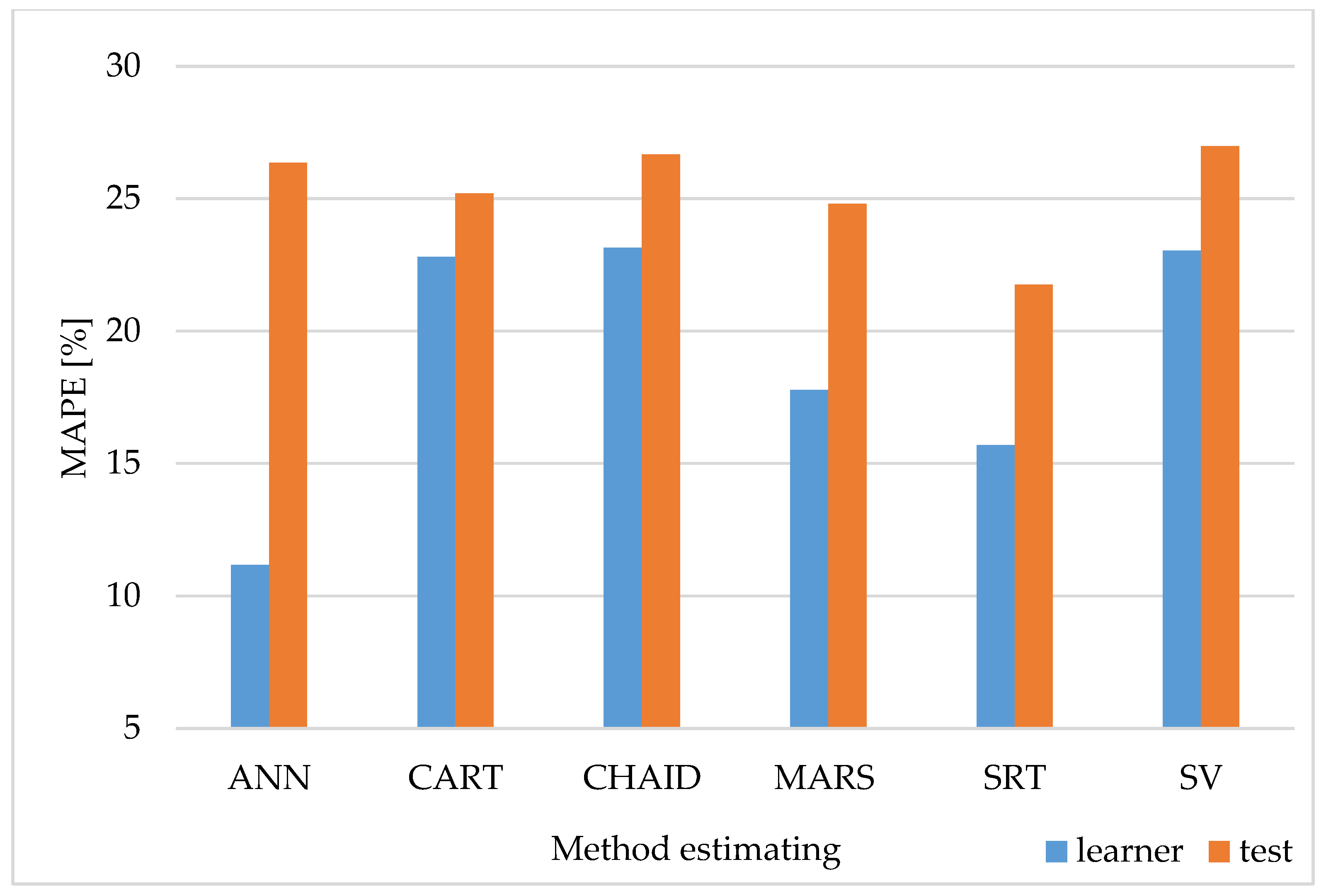
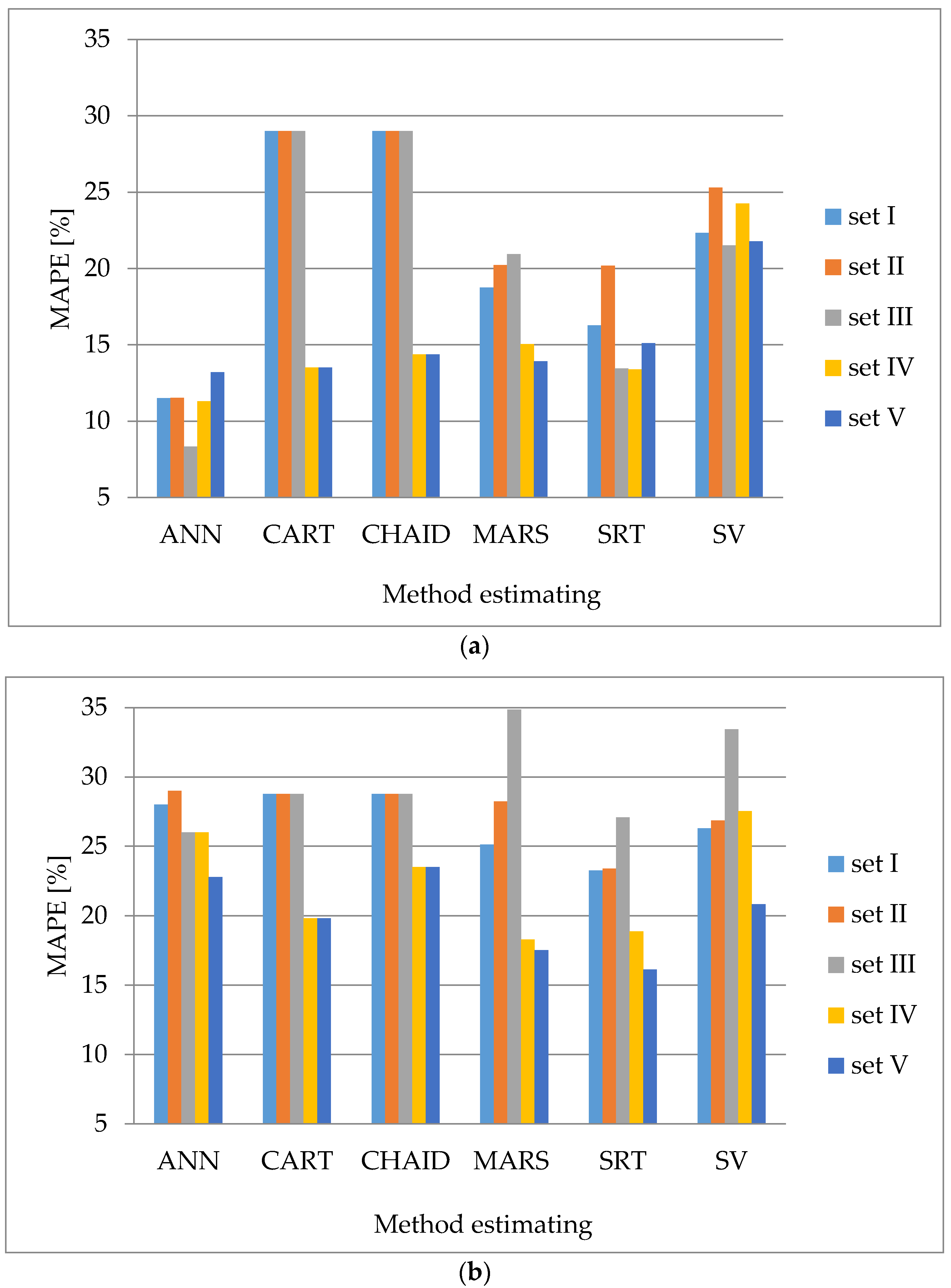
5. Results and Discussion

The results obtained for particular models (for the learning and test set) depending on the selected set of input variables are presented in Figure 5 and Figure 6.

The analysis carried out for artificial neural network methods shows that the lowest error MAPE when estimating the reduction of the energy requirement in a building after the completion of the thermomodernization designated for the learners irrespective of the selected set of input variables is expected. However, this method characterized a relatively high error of forecast (26%) set on test data not participating in network learning. A very promising result was obtained for the support regression trees (SRT) method. For the collection of learners, the error for this method was more than 5% higher than the ANN, but on the data that is a test collection allowed to most relevant predictions risky a map error of less than 22%. Based on the analysis of the quality assessment indicators, further analysis will also include the MARS method but only for selected sets of independent variables. The worst methods in the comparative analysis were: general regression trees (CART), exhaustive regression trees (CHAID) and support vectors (SV), and the error values of the MAPE oscillated between 23% and 27% (Figure 5).

In the next part of the work, studies were performed to see how the selection of the input variable set affects the quality of the forecasts analyzed by methods. Figure 6 shows error values for all methods depending on the set of input variables.

The analysis performed shows that the best quality forecasts regardless of the method selection can be obtained for the fourth and fifth sets of variables. The only exception for the ANN, SRT and SV method was the third set that the data in the learner collection generated the best quality forecasts, but the error was higher than for the other sets of variables on the test collection (Figure 6). For this reason, in the remainder of the work, this kit was not analyzed.

In order to get the lowest possible errors, the energy consumption forecasts in multi-family buildings after thermomodernization can be obtained using the support regression trees (SRT) method and the MARS method, for which as variables input uses variables selected for the IV and V set of independent variables.

The quality assessment of the developed models was not only based on the MAPE error analysis, but was extended by the price of MBE, CV RMSE, and R². The indicators were selected based on ASHRAE Guideline 14 [41,42] and the Federal Energy Management Program FEMP criteria [43].

Table 3. Comparison of the Mean Bias Error (MBE), Coefficient of Variation of the Root Mean Square Error) (CV RMSE), coefficient of determination (R²), of selected methods estimating the reduction energy requirement taking into account all accessibles input variables for test.

Index	Set	Method Estimating
		ANN	CART	CHAID	MARS	SRT	SV
MBE [%]	I	12.9	8.7	8.7	14.3	9.9	8.6
	II	9.5	8.7	8.7	8.7	5.6	7.9
	III	8.8	8.7	8.7	18.4	12.2	14.0
	IV	4.0	9.5	4.0	4.0	4.7	2.8
	V	4.0	9.5	4.0	6.0	6.0	1.7
CV RMSE [%]	I	23.8	28.1	28.1	29.7	27.5	26.1
	II	23.8	28.1	28.1	33.9	25.7	26.8
	III	20.5	28.1	28.1	37.4	27.0	39.4
	IV	13.7	20.7	24.6	14.8	13.9	28.4
	V	13.7	20.7	24.6	17.8	16.4	20.7
R2	I	0.6	0.3	0.3	0.4	0.4	0.4
	II	0.6	0.3	0.3	0.3	0.4	0.3
	III	0.7	0.3	0.3	0.3	0.4	0.1
	IV	0.8	0.7	0.4	0.8	0.8	0.3
	V	0.8	0.7	0.4	0.7	0.8	0.6

presents the MBE, CV RMSE and R² evaluation indicators for selected methods of estimating energy demand reduction taking into account all available input variables.

The MBE value assesses the absolute differences between the value obtained from the developed model and the actual value. It can take both positive and negative values. According to the evaluation criteria [41,42,43], the value of this indicator should amount to ±5. The results of the study (Table 3) show that on the test set the MBE value for all evaluated models and analyzed sets of variables was positive. Thus, the models developed underestimate the estimated reduction of energy demand in buildings undergoing thermal upgrading. For most models, for which the input variables constituted the fourth and fifth set of variables, the index values were very low and oscillated around 2–4%. This indicator is commonly used to assess the quality of the model, but it has a certain disadvantage, because in case of positive and negative values, the total value decreases significantly.

To assess the quality of the models built, CV RMSE index was therefore used, where there is no error cancellation problem caused by changing the index sign (positive with negative). According to the criteria the Federal Energy Management Program (FEMP) and ASHRAE Guideline 14 the index value should not exceed 20–30% for hourly data and 15% for monthly data [41,42,43]. The paper assumes that correctly calibrated models are to have a coefficient of variation of the square root mean error at a level not higher than 15%. The analysis shows that this assumption is fulfilled by the ANN model for the IV and IV set of variables and the MARS and SRT models for the IV set of variables.

ASHRAE Guideline 14 also recommends assessing the quality of the model based on the analysis of the coefficient of determination R² and to take 0.75 as a minimum value for well calibrated models. This requirement has been met by ANN, MARS and SRT models for 4 and 5 sets of variables, just as for the previously analysed indicators (Table 3).

6. Conclusions and Perspectives

Based on analyses carried out on a group of several hundred residential buildings in a four-season climate, for which the authors of the study developed energy audits, specific sets of deliberately selected variables characterizing the buildings were distinguished. The variables are grouped into five sets depending on the strength of impact on energy consumption after thermal renovation and difficulties in obtaining them. The first two collections use the indicators most closely correlated with the energy consumption of the building. These variables were divided into two sets because the independent variables were strongly correlated with each other. In the next sets it was analyzed how extending the variables with information related to the structural and thermal parameters of the building will affect the quality of the models. The models developed in the future will allow for a quick determination of the energy saving potential after the completion of the thermal modernization for buildings made using large plate technology (prefabricated).

• When assessing the quality of individual methods solely on the basis of the MAPE index (the index most frequently used for assessment) determined for the test set, it can be said that the best quality energy consumption forecasts after thermal rehabilitation were obtained by SRT and ANN methods, for which it was necessary to use the data from the V set as input variables. The error value was 12.1% and 12.5% respectively. Slightly worse quality forecasts, because they were burdened with a MAPE error of 14%, were obtained for the IV set of input variables and methods ANN, MARS, and SRT.
• When evaluating the methods according to the indicators proposed by ASHARE, the SV model together with IV and V sets of input variables should be considered the best in terms of MBE error. Slightly worse results, at the error level of about 4%, were obtained for the two best methods in terms of MAPE error, i.e., ANN and SRT and CHID and MARS methods. Unfortunately, CHID and SV methods were characterized by twice as high RMSE CV error as the other indicated methods. Also, the correlation coefficient for them did not meet the assumed assumptions, as it was only 0.3–0.6.
• Taking into account all quality assessment indicators, the ANN models should be indicated as preferred, together with an IV or V set of independent variables. For these sets of variables, the use of SRT models, followed by MARS, can also be considered. These models were in most cases burdened with only slightly larger errors.

In the future, the studied group of objects will be used to test other forecasting methods, e.g., hybrid methods (combining artificial neural networks and fuzzy logic), so that research results can be compared with each other. In further research, the authors also plan to test the usefulness of these methods for forecasting energy consumption in other types of buildings, such as schools, kindergartens, and others.

References

1. Reckel, P. Effet de Serres Sur le €O2. 2040 Quel Climat en France Métropolitaine; Amazon: Paris, France, 2019. [Google Scholar]
2. Frezal, B.; Leininger-Frezal, C.; Mathia, T.G.; Mory, B. Influence et Systèmes–Introduction Provisoire à la Théorie de L’Influence et de la Manipulation; L’Interdisciplinaire: Québec, QC, Canada, 2011. [Google Scholar]
3. Bourdeau, M.; Zhai, X.-Q.; Nefzaoui, E.; Guo, X.; Chatellier, P. Modelling and forecasting building energy consumption: A review of data-driven techniques. Sustain. Cities Soc. 2019, 48, 101533. [Google Scholar] [CrossRef]
4. Dong, B.; Li, Z.; Rahman, S.M.M.; Vega, R. A hybrid model approach for forecasting future residential electricity consumption. Energy Build. 2016, 117, 341–351. [Google Scholar] [CrossRef]
5. ASHRAE. ASHRAE Handbook–Fundamentals—Energy Estimation and Modeling Methods, 6th ed.; American Society of Heating, Refrigerating and Air-Conditioning Engineers, Inc. (ASHRAE): Atlanta, GA, USA, 2009; ISBN 978-1-61583-170-8. Available online: https://app.knovel.com/web/toc.v/cid:kpASHRAE37/viewerType:toc/ (accessed on 5 November 2019).
6. Zhao, H.; Magoulès, F. A review on the prediction of building energy consumption. Renew. Sustain. Energy Rev. 2012, 16, 3586–3592. [Google Scholar] [CrossRef]
7. Szul, T.; Kokoszka, S. Application of Rough Set Theory (RST) to forecast energy consumption in buildings undergoing thermal modernization. Energies 2020, 13, 1309. [Google Scholar] [CrossRef] [Green Version]
8. CEN. Energy Performance of Buildings. Ventilation for Buildings. Indoor Environmental Input Parameters for Design and Assessment of Energy Performance of Buildings Addressing Indoor Air Quality, Thermal Environment, Lighting and Acoustics. Module M1-6; ISO 16798-1:2019-06. Available online: https://standards.globalspec.com/std/14317955/bs-en-16798-1-tc (accessed on 23 September 2020).
9. Costanzoa, V.; Fabbrib, K.; Piraccini, S. Stressing the passive behavior of a Passivhaus: An evidence-based scenario analysis for a Mediterranean case study. Build. Environ. 2018, 142, 265–277. [Google Scholar] [CrossRef]
10. Djamila, H. Indoor thermal comfort predictions: Selected issues and trends. Renew. Sustain. Energy Rev. 2017, 74, 569–580. [Google Scholar] [CrossRef]
11. Wang, Y.; Kuckelkorn, J.; Zhao, F.-Y.; Spliethoff, H.; Lang, W. A state of art of review on interactions between energy performance and indoor environment quality in Passive House buildings. Renew. Sustain. Energy Rev. 2017, 72, 1303–1319. [Google Scholar] [CrossRef]
12. CEN. European Standard: Energy Performance of Buildings-Calculation of Energy Use for Space Heating and Cooling; ISO 13790:2008. 2008. Available online: https://www.iso.org/standard/41974.html (accessed on 5 November 2019).
13. CEN. European Standard: Heating Systems in Buildings; ISO 12831-1:2017-08. 2017. Available online: https://sklep.pkn.pl/pn-en-12831-3-2017-08e.html (accessed on 17 November 2019).
14. Ballarini, I.; Corrado, V. Application of energy rating methods to the existing building stock. Analysis of some residential buildings in Turin. Energy Build. 2009, 4, 790–800. [Google Scholar] [CrossRef]
15. Crawley, D.B.; Lawrie, L.K.; Winkelmann, F.C.; Buhl, W.F.; Huang, Y.J.; Pedersen, C.O.; Strand, R.K.; Liesen, R.J.; Fisher, D.E.; Witte, M.J.; et al. Energyplus: Creating a new-generation building energy simulation program. Energy Build. 2001, 33, 319–331. [Google Scholar] [CrossRef]
16. Rivers, N.; Jaccard, M. Combining top-down and bottom-up approaches to energy–economy modeling using discrete choice methods. Energy J. 2005, 26, 83–106. [Google Scholar] [CrossRef] [Green Version]
17. Allard, I.; Olofsson, T.; Hassan, O.A.B. Methods for energy analysis of residential buildings in Nordic countries. Renew. Sustain. Energy Rev. 2013, 22, 306–318. [Google Scholar] [CrossRef]
18. Asadi, S.; Amiri, S.S.; Mottahedi, M. On the development of multi-linear regression analysis to assess energy consumption in the early stages of building design. Energy Build. 2014, 85, 246–255. [Google Scholar] [CrossRef]
19. Asadi, S.; Marwa, H.; Beheshti, A. Development and validation of a simple estimating tool to predict heating and cooling energy demand for attics of residential buildings. Energy Build. 2012, 54, 12–21. [Google Scholar] [CrossRef]
20. Caldera, M.; Corgnati, S.P.; Filippi, M. Energy demand for space heating through a statistical approach: Application to residential buildings. Energy Build. 2008, 40, 1972–1983. [Google Scholar] [CrossRef]
21. Chou, J.S.; Bui, D.K. Modeling heating and cooling loads by artificial intelligence for energy-efficient building design. Energy Build. 2014, 82, 437–446. [Google Scholar] [CrossRef]
22. Fumo, N.; Biswas, R. Regression analysis for prediction of residential energy consumption. Renew. Sustain. Energy Rev. 2015, 47, 332–343. [Google Scholar] [CrossRef]
23. Lü, X.; Lu, T.; Kibert, C.J.; Viljanen, M. Modeling and forecasting energy consumption for heterogeneous buildings using a physical–statistical approach. Appl. Energy 2015, 144, 261–275. [Google Scholar] [CrossRef]
24. Ma, Z.; Li, H.; Sun, Q.; Wang, C.; Yan, A.; Starfelt, F. Statistical analysis of energy consumption patterns on the heat demand of buildings in district heating systems. Energy Build. 2014, 85, 464–472. [Google Scholar] [CrossRef]
25. Praznik, M.; Butala, V.; Zbašnik-Senegačnik, M. Simplified evaluation method for energy efficiency in single-family houses using key quality parameters. Energy Build. 2013, 67, 489–499. [Google Scholar] [CrossRef]
26. Sekhar-Roy, S.; Roy, R.; Balas, V.E. Estimating heating load in buildings using multivariate adaptive regression splines, extreme learning machine, a hybrid model of mars and elm. Renew. Sustain. Energy Rev. 2018, 82, 4256–4268. [Google Scholar] [CrossRef]
27. Tiberiu, C.; Virgone, J.; Blanco, E. Development and validation of regression models to predict monthly heating demand for residential buildings. Energy Build. 2008, 40, 1825–1832. [Google Scholar] [CrossRef]
28. Tsanas, A.; Xifara, A. Accurate quantitative estimation of energy performance of residential buildings using statistical machine learning to OLS. Energy Build. 2012, 49, 560–567. [Google Scholar] [CrossRef]
29. Biswas, M.; Robinson, M.D.; Fumo, N. Prediction of residential building energy consumption: A neural network approach. Energy 2016, 117, 84–92. [Google Scholar] [CrossRef]
30. Breiman, L.; Friedman, J.H.; Olshen, R.A.; Stone, C.J. Classification and Regression Trees; Wadsworth & Brooks/Cole Advanced Books & Software: Monterey, CA, USA, 1984. [Google Scholar]
31. Ekici, B.B.; Aksoy, U.T. Prediction of building energy consumption by using artificial neural networks. Adv. Eng. Softw. 2009, 40, 356–362. [Google Scholar] [CrossRef]
32. Li, K.; Sua, H.; Chua, J. Forecasting building energy consumption using neural networks and hybrid neuro-fuzzy system: A comparative study. Energy Build. 2011, 43, 2893–2899. [Google Scholar] [CrossRef]
33. Kumar, R.; Aggarwal, R.K.; Sharma, J.D. Energy analysis of a building using artificial neural network: A review. Energy Build. 2013, 65, 352–358. [Google Scholar] [CrossRef]
34. Seyedzadeh, S.; Rahimian, F.; Glesk, I.; Roper, M. Machine learning for estimation of building energy consumption and performance: A review. Vis. Eng. 2018, 6, 5. [Google Scholar] [CrossRef]
35. Ripley, B.D. Pattern Recognition and Neural Networks; Cambridge University Press: Cambridge, UK, 1996; ISBN 0-521-46086-7. [Google Scholar]
36. Kass, G.V. An exploratory technique for investigating large quantities of categorical data. Appl. Stat. 1980, 29, 119–127. [Google Scholar] [CrossRef]
37. Friedman, J. Multivariate adaptive regression splines (with discussion). Ann. Stat. 1991, 19, 1–141. [Google Scholar] [CrossRef]
38. Hastie, T.; Tibshirani, R.; Friedman, J.H. The Elements of Statistical Learning: Data Mining, Inference, and Prediction; Springer: New York, NY, USA, 2001. [Google Scholar]
39. CEN. Performance in Construction-Determination and Calculation of Surface and Volume Indicators. ISO 9836:1997. Available online: https://www.iso.org/standard/73149.html (accessed on 7 November 2019).
40. CEN. Building Components and Building Elements—Thermal Resistance and Thermal Transmittance—Calculation Methods. ISO 6946:2017-10. Available online: https://www.iso.org/standard/65708.html (accessed on 9 November 2019).
41. American Society of Heating, Ventilating, and Air Conditioning Engineers (ASHRAE). Guideline 14-2014, Measurement of Energy and Demand Savings; Technical Report; American Society of Heating, Ventilating, and Air Conditioning Engineers: Atlanta, GA, USA, 2014. [Google Scholar]
42. Ruiz, G.R.; Bandera, C.R. Validation of Calibrated Energy Models: Common Errors. Energies 2017, 10, 1587. [Google Scholar] [CrossRef] [Green Version]
43. Webster, L.; Bradford, J.; Sartor, D.; Shonder, J.; Atkin, E.; Dunnivant, S.; Frank, D.; Franconi, E.; Jump, D.; Schiller, S.; et al. M&V Guidelines: Measurement and Verification for Performance-Based Contracts; Version 4.0, Technical Report; U.S. Department of Energy Federal Energy Management Program: Washington, DC, USA, 2015.
Figure 1. Methodological Flow Chart of different tasks and relative intellectual investment and time-consuming visualization.
Energies 13 05453 g001
Figure 2. Representative image of one of few hundreds explored buildings (a) before thermomodernization and (b) its thermogram indicating heat flows.
Energies 13 05453 g002
Figure 3. Representative image of (a) one of few hundreds explored buildings and (b) its thermogram indicating residual heat flows after thermomodernization.
Energies 13 05453 g003
Figure 4. View of working space Data Miner visualizing global strategy of adopted methodology.
Energies 13 05453 g004
Figure 5. Comparison of the average quality indicators (MAPE), of selected methods estimating the reduction energy requirements for all accessible taking into account all accessible input variables (sets I–V).
Energies 13 05453 g005
Figure 6. Comparison of the average quality indicators (MAPE), of selected methods estimating the reduction energy requirement taking into account all accessible input variables versus different set’s selection for: (a) learner, (b) test.
Energies 13 05453 g006