Sky Luminance Distribution Models: A Comparison with Measurements from a Maritime Desert Region


Abstract
1. Introduction
2. All Sky Luminance Distribution Models
2.1. Perraudeau Model
2.2. Brunger Model
2.3. Harrison Model
2.4. Matsuura Model
2.5. ASRC-CIE Model (Pereze90)
2.6. Perez Model (Perez 93)
- (a)
- Darkening or brightening at the horizon.
- (b)
- Luminance gradient near the horizon.
- (c)
- Relative intensity of the circumsolar region.
- (d)
- Width of the circumsolar region.
- (e)
- The relative backscattered light.
2.7. Igawa Model
3. Luminance and Solar Radiation Measurements
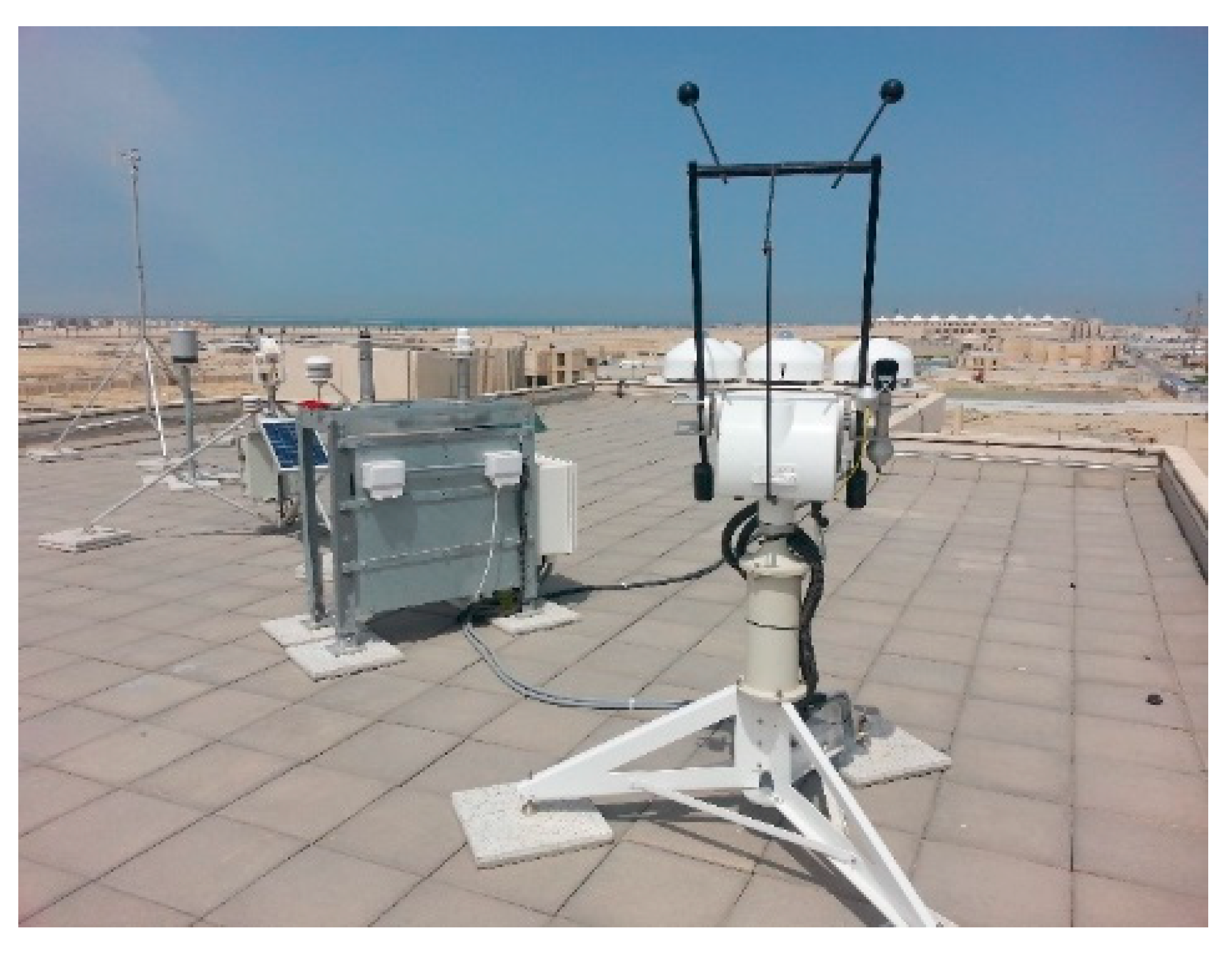
- A solar monitor station operated (Figure 2), maintained, and calibrated by King Abdullah City for Atomic and Renewable Energy [48]. The data collected from this station include: direct normal irradiance where the measurements are done with a pyrheliometer mounted in an automatic solar tracker (Solys 2—Kipp and Zonene); diffuse horizontal irradiance where the measurements are done with a shaded pyranometer (Kipp and Zonene), and global horizontal irradiance measured with an unshaded pyranometer (Kipp and Zonene).
- A newly installed EKO sky scanner model MS 321 LR (Figure 3) was used for sky luminance measurements.
- Rejecting readings of global horizontal radiation greater than 1.2 times the corresponding extraterrestrial horizontal radiation.
- Rejecting readings of horizontal sky radiation greater than 0.8 times the corresponding extraterrestrial horizontal radiation.
- Rejecting all readings when the solar altitude is less than five degrees.
- Rejecting all data when the direct normal exceeds the corresponding extraterrestrial solar component.
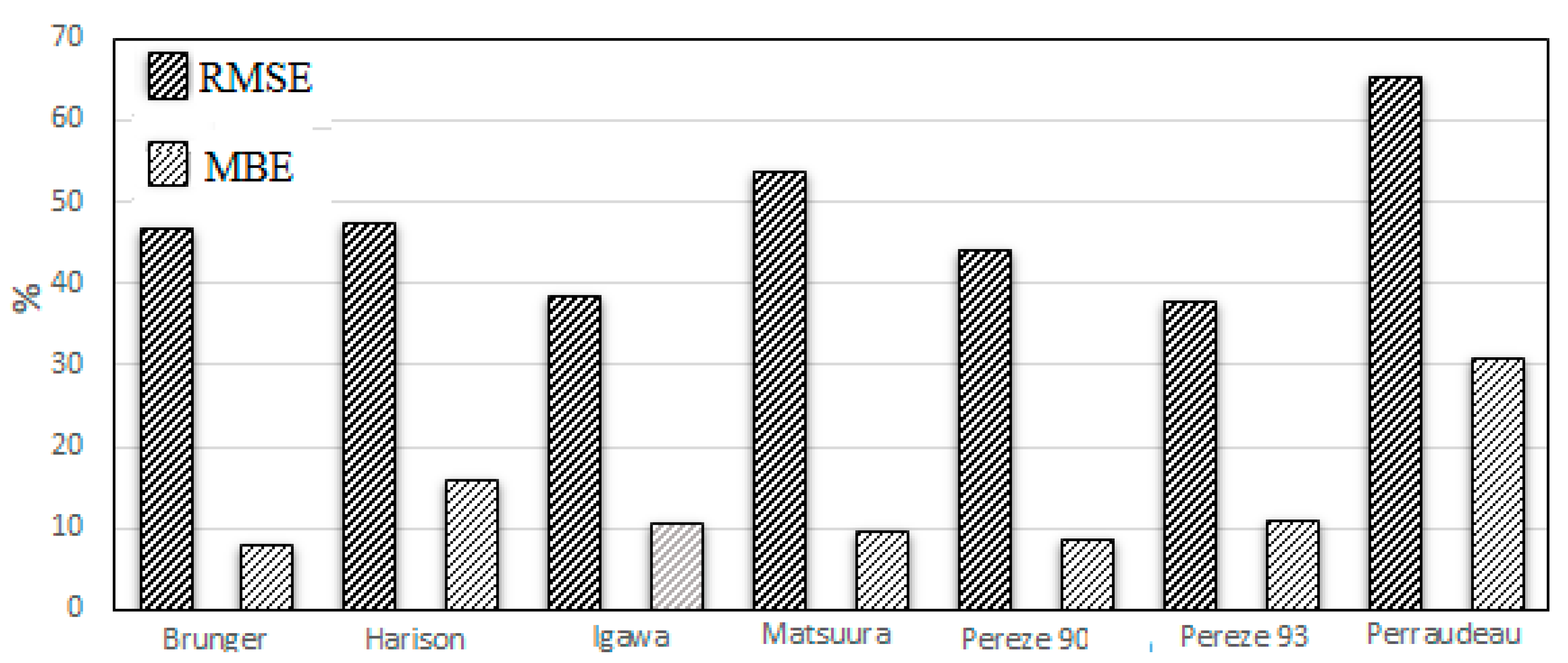
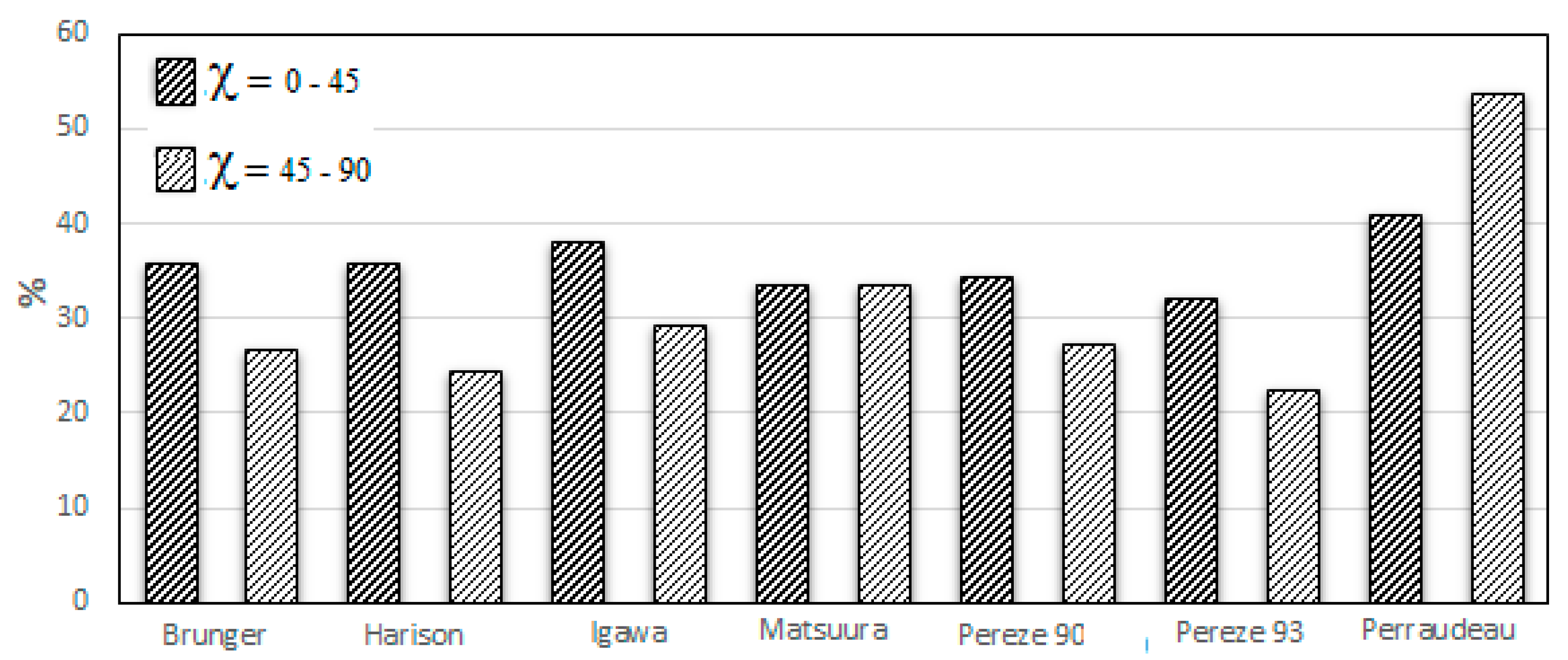
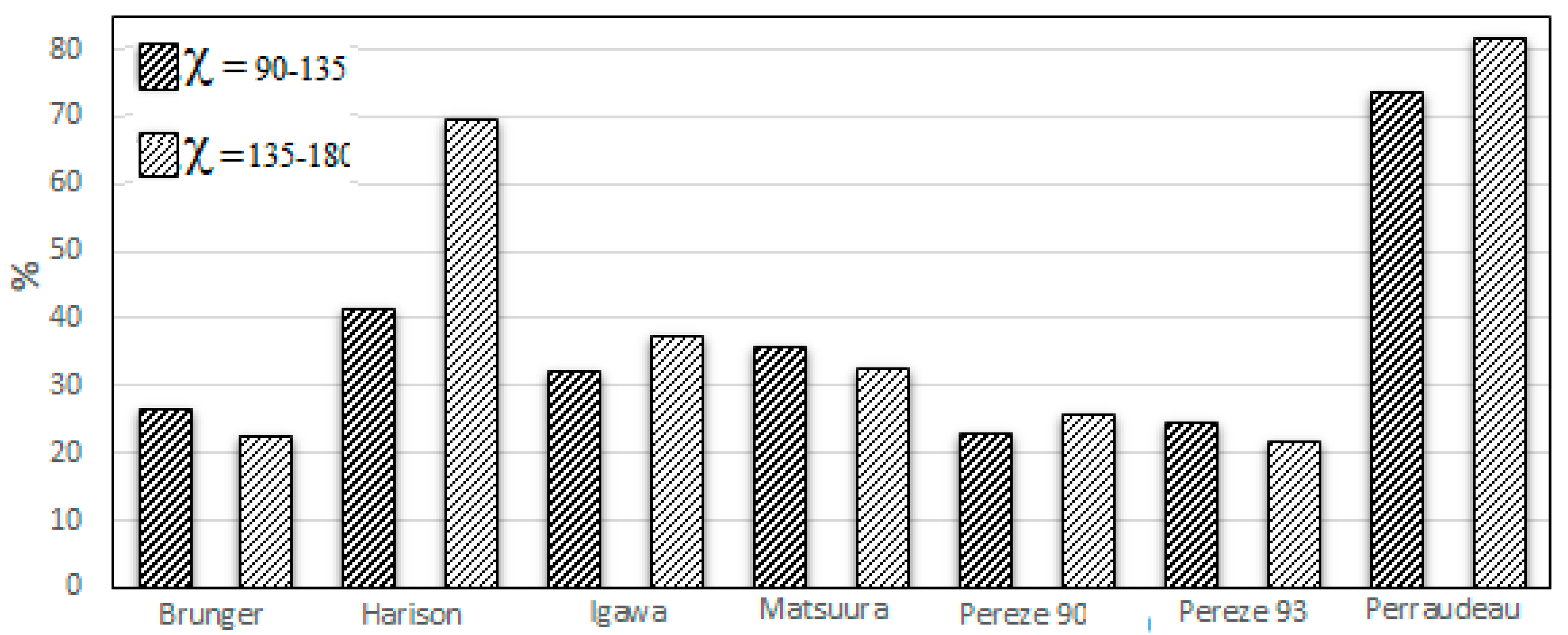
4. Results and Analysis
- Sky points within an angular distance of 45° or less from the sun.
- Sky points within an angular distance between 45° and 90° from the sun.
- Sky points within an angular distance between 90° and 135° from the sun.
- Sky points within an angular distance of more than 135° from the sun.
5. Conclusions
Author Contributions
Funding
Conflicts of Interest
Nomenclature
| C | ratio of horizontal sky radiance to global horizontal irradiance. |
| Eed | diffuse horizontal irradiance (w/m2) |
| Edvm | horizontal sky illuminance calculated from the measured 145 scan points (lux) |
| Edvp | horizontal sky illuminance calculated from the predicted 145 scan points (lux) |
| Ees | normal irradiance (w/m2) |
| Eeo | extraterrestrial normal irradiance. |
| Lcie_cl | luminance at considered point using CIE standard clear sky (Kcd/m2) |
| Lcie_ct | luminance at considered point using CIE standard clear-turbid sky (Kcd/m2) |
| Lcie_in | luminance at considered point using CIE standard intermediate Sky (Kcd/m2) |
| L cie_ov | luminance at considered point using CIE standard overcast Sky (Kcd/m2) |
| Lmi | measured luminance for scan point i (Kcd/m2) |
| Lpi | calculated luminance for scan point i (Kcd/m2) |
| Lv | luminance of a sky element (Kcd/m2). |
| Lz | zenith luminance (Kcd/m2) |
| m | optical mass |
| N | total number of scan point 145 |
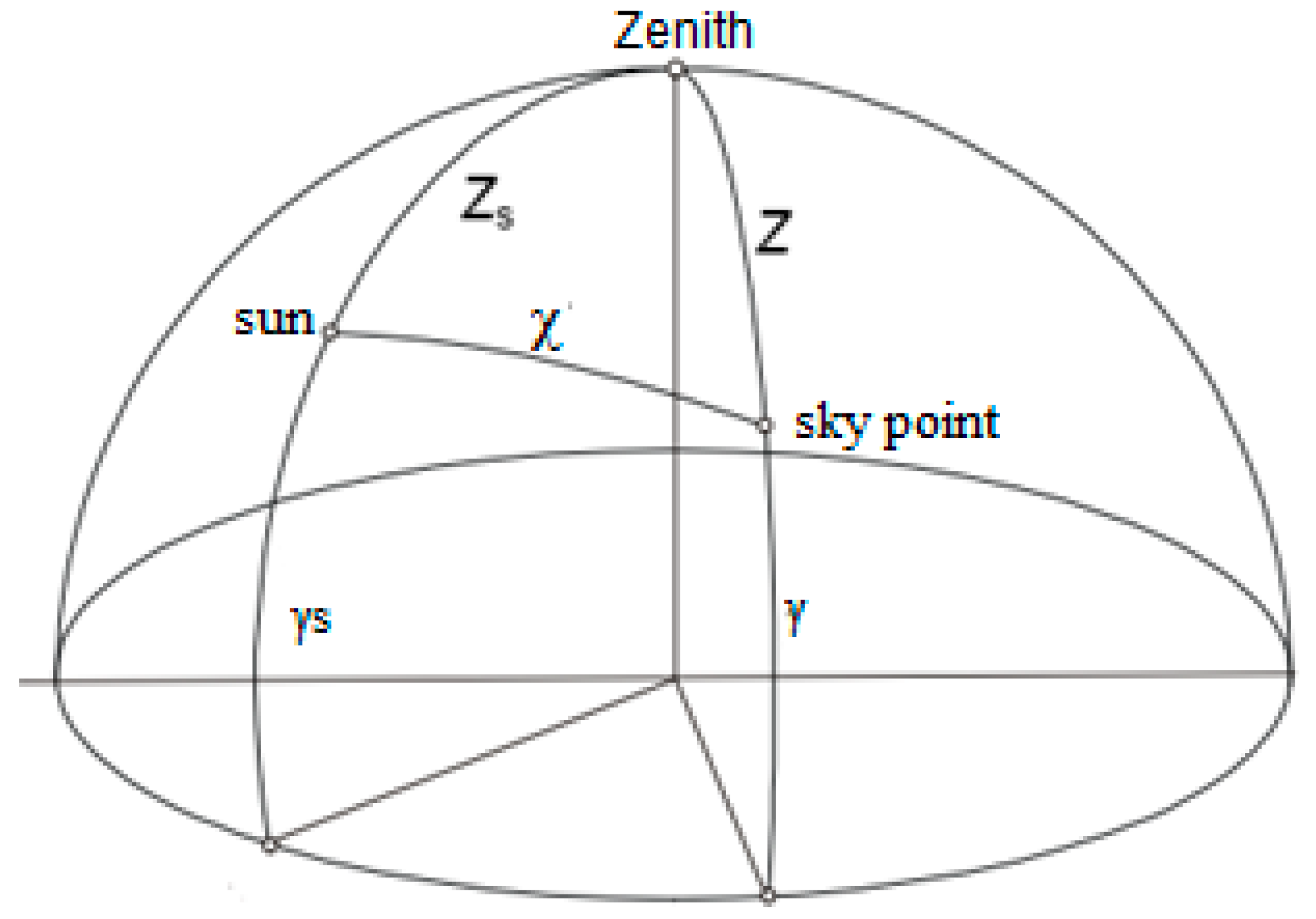
| χ | angle between the sun and the sky point. |
| Z | angle between the zenith and the sky point. |
| Zs | angle between the zenith and the sun. |
| γ | the altitude of sky point. |
| γs | the altitude of sun. |
References
- Li, D.H.W.; Tsang, E.K.W. An analysis of daylighting performance for office buildings in Hong Kong. Build. Environ. 2008, 43, 1446–1458. [Google Scholar] [CrossRef]
- Alshaibani, K. Potentiality of daylighting in a maritime desert climate: The Eastern coast of Saudi Arabia. Renew. Energy 2001, 23, 325–331. [Google Scholar] [CrossRef]
- Futrell, B.J.; Ozelkan, E.C.; Brentrup, D. Optimizing complex building design for annual daylighting performance and evaluation of optimization algorithms. Energy Build. 2015, 92, 234–245. [Google Scholar] [CrossRef]
- Collins, B.L. Review of the psychological reaction to windows. Light. Res. Technol. 1976, 8, 80–88. [Google Scholar] [CrossRef]
- Boyce, P.; Hunter, C.; Howlett, O. The Benefits of Daylight through Windows; Rensselaer Polytechnic Institute: Troy, NY, US, 2003. [Google Scholar]
- Altomonte, S. Daylight and the Occupant. Visual and Physio-psychological well-being in built environments. In Proceedings of the Plea2009—26th Conference on Passive and Low Energy Architecture, Quebec, QC, Canada, 22–24 June 2009. [Google Scholar]
- Knoop, M. Daylight: What makes the difference? Light. Res. Technol. 2020, 52, 423–442. [Google Scholar] [CrossRef]
- Aries, M.; Aarts, M.; van Hoof, J. Daylight and health: A review of the evidence and consequences for the built environment. Light. Res. Technol. 2015, 47, 6–27. [Google Scholar] [CrossRef]
- Kittler, R.; Perez, R.; Darula, S. A new generation of sky standards. Proc. Lux Eur. Amst. 1997, 1997, 359–373. [Google Scholar]
- Commission International de l’Eclairage. Spatial Distribution of Daylight—CIE Standard of General Sky, CIE Standard S 011/E: 2003; February: Viena, Austria, 2003. [Google Scholar]
- International Standard Organisation. Spatial Distribution of Daylight—CIE Standard General Sky; CIE Central Bureau: Vienna, Austria, 2004. [Google Scholar]
- Tregenza, P. Analysing sky luminance scans to obtain frequency distributions of CIE Standard General Skies. Light. Res. Technol. 2004, 36, 271–281. [Google Scholar] [CrossRef]
- Kittler, R.; Darula, S. The simultaneous occurrence and relationship of sunlight and skylight under ISO/CIE standard sky types. Light. Res. Technol. 2015, 47, 565–580. [Google Scholar] [CrossRef]
- Alshaibani, K. Finding frequency distributions of CIE Standard General Skies from sky illuminance or irradiance. Light. Res. Technol. 2011, 43, 487–495. [Google Scholar] [CrossRef]
- Alshaibani, K.A. Classification Standard Skies: The use of horizontal sky illuminance. Renew. Sustain. Energy Rev. 2017, 73, 387–392. [Google Scholar] [CrossRef]
- Li, D.H.W.; Chau, T.C.; Wan, K.K.W. A review of the CIE general sky classification approaches. Renew. Sustain. Energy Rev. 2014, 31, 563–574. [Google Scholar] [CrossRef]
- de Simón-Martín, M.; Alonso-Tristán, C.; Díez-Mediavilla, M. Diffuse solar irradiance estimation on building’s façades: Review, classification and benchmarking of 30 models under all sky conditions. Renew. Sustain. Energy Rev. 2017, 77, 783–802. [Google Scholar] [CrossRef]
- Noorian, A.M.; Moradi, I.; Kamali, G.A. Evaluation of 12 models to estimate hourly diffuse irradiation on inclined surfaces. Renew. Energy 2008, 33, 1406–1412. [Google Scholar] [CrossRef]
- Notton, G.; Poggi, P.; Cristofari, C. Predicting hourly solar irradiations on inclined surfaces based on the horizontal measurements: Performances of the association of well-known mathematical models. Energy Convers. Manag. 2006, 47, 1816–1829. [Google Scholar] [CrossRef]
- Li, D.H.W.; Lam, J.C. Evaluation of Perez slope irradiance and illuminance models against measured Hong Kong data. Int. J. Ambient. Energy 1999, 20, 193–204. [Google Scholar] [CrossRef]
- Lam, K.P.; Mahdavi, A.; Ullah, M.B.; Ng, E.; Pal, V. Evaluation of six sky luminance prediction models using measured data from Singapore. Light. Res. Technol. 1999, 31, 13–17. [Google Scholar] [CrossRef]
- Perez, R.; Michalshy, J.; Seals, R. Modeling sky luminance angular distribution for real sky conditions: Experimental evaluation of existing algorithms. J. Illum. Eng. Soc. 1992, 21, 84–92. [Google Scholar] [CrossRef]
- Chaiwiwatworakul, P.; Chirarattananon, S. Evaluation of sky luminance and radiance models using data of north Bangkok. Leukos 2005, 1, 107–126. [Google Scholar] [CrossRef]
- Jones, N.L.; Reinhart, C.F. Effects of real-time simulation feedback on design for visual comfort. J. Build. Perform. Simul. 2019, 12, 343–361. [Google Scholar] [CrossRef]
- Xiong, J.; Tzempelikos, A.; Bilionis, I.; Karava, P. A personalized daylighting control approach to dynamically optimize visual satisfaction and lighting energy use. Energy Build. 2019, 193, 111–126. [Google Scholar] [CrossRef]
- Leccese, F.; Salvadori, G.; Tambellini, G.; Kazanasmaz, Z.T. Application of climate-based daylight simulation to assess lighting conditions of space and artworks in historical buildings: The case study of Cetacean gallery of the monumental charterhouse of Calci. J. Cult. Herit. 2020, in press. [Google Scholar] [CrossRef]
- Vera, S.; Uribe, D.; Bustamante, W.; Molina, G. Optimization of a fixed exterior complex fenestration system considering visual comfort and energy performance criteria. Build. Environ. 2017, 113, 163–174. [Google Scholar] [CrossRef]
- Hosseini, S.M.; Mohammadi, M.; Rosemann, A.; Schröder, T. Quantitative investigation through climate-based daylight metrics of visual comfort due to colorful glass and orosi windows in iranian architecture. J. Daylighting 2018, 5, 21–33. [Google Scholar] [CrossRef]
- He, Y.; Zhang, X.; Quan, L. Estimation of hourly average illuminance under clear sky conditions in Chongqing. PLoS ONE 2020, 15, e0237971. [Google Scholar] [CrossRef]
- Costanzo, V.; Evola, G.; Marletta, L.; Nascone, F.P. Application of climate based daylight modelling to the refurbishment of a school building in sicily. Sustainability 2018, 10, 2653. [Google Scholar] [CrossRef]
- Zheng, C.; Wu, P.; Costanzo, V.; Wang, Y.; Yang, X. Establishment and Verification of Solar Radiation Calculation Model of Glass Daylighting Roof in Hot Summer and Warm Winter Zone in China. Procedia Eng. 2017, 205, 2903–2909. [Google Scholar] [CrossRef]
- Lou, S.; Li, D.H.W.; Huang, Y.; Zhou, X.; Xia, D.; Zhao, Y. Change of climate data over 37 years in Hong Kong and the implications on the simulation-based building energy evaluations. Energy Build. 2020, 222, 110062. [Google Scholar] [CrossRef]
- Ineichen, P.; Molineaux, B.; Perez, R. Sky luminance data validation: Comparison of seven models with four data banks. Sol. Energy 1994, 52, 337–346. [Google Scholar] [CrossRef]
- Gracia, A.; Torres, J.L.; de Blas, M.; García, A.; Perez, R. Comparison of four luminance and radiance angular distribution models for radiance estimation. Sol. Energy 2011, 85, 2202–2216. [Google Scholar] [CrossRef]
- Ferraro, V.; Mele, M.; Marinelli, V. Sky luminance measurements and comparisons with calculation models. J. Atmos. Sol. Phys. 2011, 73, 1780–1789. [Google Scholar] [CrossRef]
- Perraudeau, M. Luminance models. In Proceedings of the CIBSE National Lighting Conference, Cambridge, UK, 5–8 April 1988; pp. 291–292. [Google Scholar]
- Brunger, A.P.; Hooper, F.C. Anisotropic sky radiance model based on narrow field of view measurements of shortwave radiance. Sol. Energy 1993, 51, 53–64. [Google Scholar] [CrossRef]
- Torres, J.L.; Torres, L.M. Angular distribution of sky diffuse radiance and luminance. In Modeling Solar Radiation at the Earth’s Surface; Springer: Berlin/Heidelberg, Germany, 2008; pp. 427–448. [Google Scholar]
- Harrison, A.W. Directional sky luminance versus cloud cover and solar position. Sol. Energy 1991, 46, 13–19. [Google Scholar] [CrossRef]
- Matsuura, K.; Iwata, T. A model of daylight source for the daylight illuminance calculations on the all weather conditions. In Proceedings of the 3rd International Daylighting Conference, Moscow, Russia, 7–9 February 1990; NIISF: Moscow, Russia, 1990. [Google Scholar]
- Commission International de l’Eclairage. Standardization of the Luminance Distribution on Clear Skies; CIE: Paris, French, 1973. [Google Scholar]
- Moon, P.; Spencer, D.E. Illumination from a non-uniform sky. Illum. Eng. 1942, 37, 707–726. [Google Scholar]
- Matsuura, K. Luminance Distributions of Various reference Skies; CIE Technical Report of TC 3-09; International Commission on Illumination: Vienna, Austria, 1987. [Google Scholar]
- Perez, R.; Ineichen, P.; Seals, R.; Michalsky, J.; Stewart, R. Modeling daylight availability and irradiance components from direct and global irradiance. Sol. Energy 1990, 44, 271–289. [Google Scholar] [CrossRef]
- Perez, R.; Seals, R.; Michalsky, J. All-weather model for sky luminance distribution—Preliminary configuration and validation. Sol. Energy 1993, 50, 235–245. [Google Scholar] [CrossRef]
- Igawa, N. Improving the All Sky Model for the luminance and radiance distributions of the sky. Sol. Energy 2014, 105, 354–372. [Google Scholar] [CrossRef]
- Ullah, M.B.; Aharari, W. An analysis of climatic variables for thermal design of building in Dhahran. Arab. J. Sci. Eng. 1982, 7, 101–110. [Google Scholar]
- Zell, E.; Gasim, S.; Wilcox, S.; Katamoura, S.; Stoffel, T.; Shibli, H.; Engel-Cox, J.; AlSubie, M. Assessment of solar radiation resources in Saudi Arabia. Sol. Energy 2015, 119, 422–438. [Google Scholar] [CrossRef]
- Tregenza, P.R.; Perez, R.; Michalsky, J.; Seals, R. Guide to Recommended Practice of Daylight Measurement; Commission Internationale de l’éclairage: Vienna, Austria, 1994. [Google Scholar]
- Alshaibani, K. The use of sky luminance and illuminance to classify the CIE Standard General Skies. Light. Res. Technol. 2015, 47, 243–247. [Google Scholar] [CrossRef]
- Alshaibani, K.A. The use of horizontal sky illuminance to classify the CIE Standard General Skies. Light. Res. Technol. 2016, 48, 1034–1041. [Google Scholar] [CrossRef]
- Illuminating Engineering Society of North America (IESNA). The IESNA Lighting Handbook: Reference & Application; Illuminating Engineering Society of North America: New York, NY, USA, 2000. [Google Scholar]


| Clear (sky ratio ≤ 0.3): | 22% |
| Partly Cloudy (0.3 < sky ratio < 0.8) | 62% |
| Overcast (0.8 ≥ sky ratio): | 16% |
Publisher’s Note: MDPI stays neutral with regard to jurisdictional claims in published maps and institutional affiliations. |
© 2020 by the authors. Licensee MDPI, Basel, Switzerland. This article is an open access article distributed under the terms and conditions of the Creative Commons Attribution (CC BY) license (http://creativecommons.org/licenses/by/4.0/).
Share and Cite
Alshaibani, K.; Li, D.; Aghimien, E. Sky Luminance Distribution Models: A Comparison with Measurements from a Maritime Desert Region. Energies 2020, 13, 5455. https://doi.org/10.3390/en13205455
Alshaibani K, Li D, Aghimien E. Sky Luminance Distribution Models: A Comparison with Measurements from a Maritime Desert Region. Energies. 2020; 13(20):5455. https://doi.org/10.3390/en13205455
Chicago/Turabian StyleAlshaibani, Khalid, Danny Li, and Emmanuel Aghimien. 2020. "Sky Luminance Distribution Models: A Comparison with Measurements from a Maritime Desert Region" Energies 13, no. 20: 5455. https://doi.org/10.3390/en13205455
APA StyleAlshaibani, K., Li, D., & Aghimien, E. (2020). Sky Luminance Distribution Models: A Comparison with Measurements from a Maritime Desert Region. Energies, 13(20), 5455. https://doi.org/10.3390/en13205455