Abstract
Soft open points (SOPs) are power electronic devices that replace the normal open points in active distribution systems. They provide resiliency in terms of transferring electrical power between adjacent feeders and delivering the benefits of meshed networks. In this work, a multi-objective bilevel optimization problem is formulated to maximize the hosting capacity (HC) of a real 59-node distribution system in Egypt and an 83-node distribution system in Taiwan, using distribution system reconfiguration (DSR) and SOP placement. Furthermore, the uncertainty in the load is considered to step on the real benefits of allocating SOPs along with DSR. The obtained results validate the effectiveness of DSR and SOP allocation in maximizing the HC of the studied distribution systems with low cost.
1. Introduction
Renewable energy integration has been crucial in recent decades to limit the effect of green-house gases on the environment [1,2,3]. Various strategies have been adopted in the modern smart grids to increase their capabilities to accommodate the intermittent renewable resources [4,5,6]. Hosting capacity (HC) is the mathematical expression that represents the ability of a distribution system to host distributed generation (DG) without violating its operational limits [5,6,7,8]. Many methodologies for improving HC [5,6,7,8] have been proposed in the literature, including power quality (PQ) enhancement, network reinforcement, distribution system reconfiguration (DSR), static var compensators (SVCs), energy storage systems (ESS), and soft open points (SOPs), among others. The maximum DG penetration was determined in [9] for the 18-node and 33-node distribution systems, considering the IEEE 519 allowable voltage harmonic limits. A constrained harmonic distortion study was carried out in [10] to maximize HC using harmonic filters. In [11], network reinforcement was employed to maximize the HC of an existing Egyptian distribution network. The deterministic HC was assessed for a real-life grid in Jordan called 73-node distribution system having a high X/R ratio, and a hypothetical grid having a lower X/R ratio called 19-node distribution system designed based on the Jordanian standards [12]. The HC was successfully maximized in [12] via two strategies, including network reinforcement and reactive power control. DSR was employed in [13] to maximize the HC of the 33-node distribution system using linear load flow formulation. HC was successfully enhanced in [14] via DSR and ESS for a real distribution system in central Italy, including 5 feeders and 287 busbars. A multi-period DSR was employed in [15,16] to enhance the HC of the IEEE 123-node and 1001-node distribution systems. Static and dynamic DSR were investigated in [17], and a static reconfiguration was found to be beneficial at the planning stage. In contrast, dynamic reconfiguration was found to be useful for active distribution networks, especially when a higher number of remotely controlled switches are available. DSR was employed in [18] to maximize HC by selecting the best configurations of the distribution network capable of maximizing the HC of a large distribution network in Japan including 235 switches. A stochastic optimization was developed in [19] for the optimal allocation of SVCs to maximize PV penetration while considering uncertainties related to photovoltaics (PVs) and loads. Quadratic power control for a central battery storage system was proposed in [20] to optimize the penetration of rooftop PVs. In [21], a linearized power flow model was formulated to determine the maximum HC of a 33-node distribution system while considering the load uncertainty. A probabilistic optimization approach was proposed in [22] to assess the effects of uncertainties on HC, while in [23], a strengthened second-order cone programming problem was formulated to maximize the HC of a 33-node distribution system using SOPs to replace tie-lines with fixed locations. An algorithm was proposed in [24] to assess the increase in the HC of a generic distribution system for SOP placement in the UK. HC has also been evaluated for various types of SOP placement, including two-terminal and multi-terminal SOPs and SOPs with energy storage [25]. In these previous works, individual strategies were employed to maximize the HC of the distribution systems, but SOPs and DSR were not combined. In the present work, we put forward a novel approach for HC enhancement based on simultaneous SOP allocation and DSR to step on the benefits of the meshed networks in the presence of load uncertainties for two real distribution systems and also ensuring the radial structure while reconfiguring the non-SOP tie-lines which provide resiliency in allocating DGs. The main contributions of this work can be summarized as follows:
- (1)
- A multi-objective bilevel optimization problem is formulated to minimize the total active losses by introducing DSR to a lower level problem and then to maximize the HC and minimize the annual total cost for two real distribution systems.
- (2)
- A probabilistic HC maximization approach is proposed to illustrate the expected impact of load uncertainties on HC.
- (3)
- The proposed optimization approach ensures radiality among the studied distribution networks while reconfiguring the non-SOP tie-lines in a short time.
- (4)
- A combination of DSR and SOPs is successfully used to support the penetration of DGs in distribution systems while guaranteeing an economic planning framework.
The rest of this paper is organized as follows: Section 2 presents the problem statement, including the power flow equations, DSR methodology, DG, and SOP models. Section 3 introduces the problem formulation. Section 4 presents the obtained results and a discussion, while Section 5 contains the conclusions and identifies future work in this area.
2. Materials and Methods
In this section, the DSR algorithm, the power flow equations, DG, and SOP modeling are illustrated in detail. Figure 1 provides an overview of DG and SOP modeling in a distribution system.
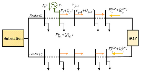
Figure 1.
Distribution system modeling.
2.1. Power Flow Equations
The power flow equations required to solve the distribution system under study are formulated as follows [26]:
where is the set of nodes of the distribution system and is the total number of nodes in the distribution system. is the impedance of the bth line joining nodes and , and its real and imaginary components are and , respectively. is the apparent power injected at the jth node, where and are its real and imaginary components, respectively. is the jth node voltage. is the demanded active power at node .
2.2. Distribution System Reconfiguration
The graph theory-based DSR algorithm proposed by the current authors in [26] is employed in this work. This method is based on a graphical interpretation of the nodes (vertices) and lines (edges) of the distribution system. The primary advantage of this DSR method is that it gives the global/near-global solution within a short time for large distribution systems. The search procedure used to optimize the current best configuration of the distribution system (), hinges on fetching the various possibilities for exchanging the yth tie-line () included in the set of the tie-lines () with its neighboring sectionalized lines, connected to its “From” (), and “To” () nodes, as shown in Figure 2. Then, the candidate sectionalized lines required to be tie-lines are sorted in a descending order via an index called weighted voltage deviation index (), where the for the Eth sectionalized line () connected to the yth tie-line is calculated as follows:
such that, and are the “From” and the “To” ends of the line . Further, at this step, a loop starts here till finding a better configuration for the distribution network having the best fitness value, where a temporary test vector () equals to is initialized. Then, the loop continues by changing the open/close status of each tie-line and its neighboring sectionalized line in . Various tests are done to ensure radiality while compiling this loop, including (1) if the power flow did not converge, thus, is not radial because of the failure in one or more of the connected loads as shown in trail #2 in Figure 2, or (2) if a better objective function value is obtained, is updated to and the loop is terminated, or (3) the loop terminates, if no possibility for exchanging the tie-lines with their neighboring lines. This algorithm was tested on various real and large distribution networks up to the 4400-node distribution system, including 185 tie-lines, and has proven its ability to ensure radiality and fast convergence toward finding the best configuration in a short time, since it directly exchanges the existing tie-lines with its neighboring sectionalized lines, thus no randomness exists.
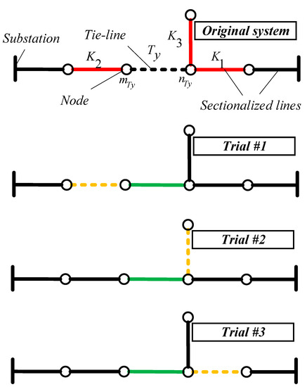
Figure 2.
Possible trails to exchange the tie-line with its neighboring lines, including , , and .
2.3. DG Modeling
In this study, the DG power factor is unity, where the power injected by the uth DG in the deterministic case study is formulated as follows:
where as for the probabilistic case study at the sth scenario:
and its allocation is constrained by the binary variables and in the deterministic and probabilistic cases, respectively, where and are equal to one in the case of DG allocation at the node. is the maximum size of the installed DGs. is the set of all scenarios studied.
2.4. SOP Modeling
SOPs were introduced in 2011 as a resilient alternative to normally open points (NOPs) and can provide the flexibility of meshed networks in sharing active and reactive power between adjacent feeders in active distribution systems [27]. SOPs may have several integration topologies, including the back-to-back voltage source converter (VSC), static series synchronous compensator (SSSC), and unified power flow controller (UPFC) [28]. In this work, the back-to-back VSC is used because of its ability to improve operational and power quality indices [29].
In this paper, two case studies are conducted to maximize the HC of real distribution systems using DSR and SOPs placement, including the deterministic and the probabilistic case studies. In both cases, the SOP is placed instead of a certain tie-line, providing resiliency in delivering apparent powers between the SOP terminals. Regulating equations for SOPs are provided below for the deterministic and probabilistic cases.
2.4.1. Deterministic Case
An SOP is allocated if its allocation variable is equal to one, and is not assigned if is equal to zero. Each tie-line is connected to either two feeders or loop laterals, the first of which is denoted by and the other by . Thus, the Ith feeder connected to the yth tie-line is denoted by .
SOP Equality Constraint [29]:
SOPs are characterized by their ability in transferring the active powers between the adjacent feeders (i.e., and feeders), where the sum of the injected SOP powers to the Ith and Jth feeders equals to zero in case of lossless SOP placement [29], whereas lossy SOP is represented in (7), where the internal active loss of the two VSCs is considered as follows [29,30]:
SOP Capacity Limit Constraint [29,30]:
Each SOP is composed of two VSCs. These VSCs are connected back-to-back through a DC-link capable of transferring both active and reactive powers constantly, and their governing equations are formulated as follows [29,30]:
where, and + are the sending and receiving transferred complex apparent powers by the SOP installed instead of the tie-line , respectively. and are the active losses by each VSC [29,30].
To limit the allocated SOP size instead of the yth tie-line, the following capacity constraint is formulated as follows [29,30]:
where, is the maximum SOP size.
SOP Internal Power Loss Equations [29]:
is the loss coefficient of each VSC [29,30]. is the total SOP losses, and is the number of SOPs installed.
2.4.2. Probabilistic Case
In this case, a set of scenarios are applied to the distribution systems, where is the total number of scenarios.
SOP Equality Constraint [29]:
SOP Capacity Limit Constraint [29]:
In addition to the capacity constraints demonstrated in (10), and (11), the following constraints expressed in (16), and (17) are considered in this case study.
SOP Internal Power Loss Equations [29]:
2.5. Scenario Reduction
In this work, the load uncertainties are represented by a preset number of scenarios, each of which has a certain corresponding probability. The 8760 hourly data are reduced to a relevant set of scenarios using the backward reduction technique developed by Growe-Kuska et al. in 2003 for stochastic programming [31].
3. Problem Formulation
In this work, a multi-objective bilevel optimization problem is developed to maximize HC and minimize the total annual cost () as the upper-level problem, whereas the lower-level problem is dedicated to minimization of the energy loss cost () using DSR. consists of the capital cost for SOP installations (), the annual operational cost of the SOPs (), and the annual total loss cost () [30].
where is the total active demand power for the distribution system under normal loading conditions, is the electricity price, is the interest rate, is the number of years, is the SOP capital cost per unit capacity, and is the SOP annual operation cost coefficient.
The solution procedure of the proposed optimization problem starts by inserting DGs at specific DG nodes (indicated by ), and SOPs instead of specific candidate tie-lines (indicated by ) at the upper level, then the rest of the tie-lines (non-SOP tie-lines) are changed at the lower level by the DSR algorithm to minimize , as a result, the power loss minimization is improved and hence choosing the best tie-lines locations for the next planning stage at the upper level. At the end of the optimization process, the technique for order of preference by similarity to ideal solution (TOPSIS) [32] algorithm takes place to choose the best solution (alternative) among the Pareto solutions, including the HC and the total annual cost quantities by a ratio of 75% and 25%, respectively.
3.1. Deterministic HC
For the deterministic case, the total power loss () is formulated as follows:
where, is the magnitude of the current passing through the bth line and is the total number of lines.
3.1.1. Upper Level
At this level, a multi-objective optimization problem is formulated to maximize HC and minimize . The objective functions are formulated as follows:
subject to (1)–(3), (5), (7)–(13), and the following operational limits:
where is the hosting capacity, and are the upper and lower voltage limits of the jth node, respectively. is the thermal current limit for the bth line. is the set of lines. is the active power delivered from the substation.
3.1.2. Lower Level
The objective function () at this level aims to minimize by DSR to obtain the best operational point. The objective function is expressed as follows:
subject to (1)–(4), (26)–(27), and (29)–(31).
3.2. Probabilistic HC
In this case, the optimization problem is solved for several different scenarios . The expected total annual energy loss () and the probabilistic HC () are expressed as follows:
where is the magnitude of the current in the sth scenario. is the bth line resistance at the sth scenario. is the total SOPs losses in the sth scenario. is the probability of the sth scenario. The bilevel multi-objective optimization for this case is formulated as follows:
3.2.1. Upper Level
At this level, the objective function is maximized and is minimized subject to (1)–(3), (6), (10)–(11), (15)–(19), (33)–(35), and the following constraints:
where, is the magnitude of the jth node, at the sth scenario. is the injected power to the slack node, at the sth scenario.
3.2.2. Lower Level
At this level, the objective function is minimized using DSR subject to (1)–(4), (26)–(27), and (36)–(38).
The interaction between the upper and the lower optimization problems during the solution of the current case study is illustrated as follows:
Step 1: Initialize the multi-objective optimization problem at the upper level, including the number of populations, number of iterations, also, the number of decision variables is given and their upper and lower limits.
Step 2: Input the optimization parameters, including , , , , , , , , , and .
Step 3: Set SOPs locations according to .
Step 4: For each scenario.
- (a)
- Apply the sth loading level to the connected loads.
- (b)
- Set DGs locations according to .
- (c)
- If (1)–(3), (6), (10),(11), (15)–(17), and (36)–(38) violated, then return , and equal to infinity, and zero, respectively. Then, the optimization process continues by setting new parameters’ values at Step 2.
- (d)
- Set the DGs, and SOPs injected powers.
- (e)
- Run the power flow.
- (f)
- The lower level optimization procedure takes place at this sub-step by reconfiguring the non-SOP tie-lines.
- (g)
- Repeat Step 4 till finishing all the scenarios.
Step 5: Evaluate , , , ,, and . After that, if the number of iterations is reached, jump to Step 6; otherwise, the upper-level optimization sets new parameters’ values and continues from Step 2.
Step 6: Deploy the TOPSIS algorithm to choose the best solution (alternative) among the Pareto-solutions according to the criterion that prefers against by a ratio of 3:1.
4. Results and Discussion
In this paper, a real 59-node distribution system in Cairo [33] and the 83-node distribution system [26] are used as test systems, shown in Figure 3 and Figure 4, respectively. The input data configurations used for the upcoming case studies are provided in Table 1. In the subsequent case studies, three multi-objective optimization techniques are employed to solve the upper-level optimization problem: the non-dominated sorting genetic algorithm (NSGA-II) [34], multi-objective particle swarm optimization (MOPSO) [35], and multi-objective multi-verse optimization (MOMVO) [36]. The authors in [34] proposed a new methodology to solve mixed-integer nonlinear programming problems via integrating the surrogate and the deterministic infeasibility sorting, where it has been tested against real-life building applications. A modified version of the MOPSO was proposed in [35] to handle multi-objective MINLP problems, where it has been tested against several benchmark functions and has proven its ability to find the best solution. In [36], Mirjalili et al. proposed a novel MOMVO for solving engineering optimization applications. It has been tested in 80 multi-objective case studies, including 49 unconstrained, 10 constrained, and 21 engineering design optimization problems.
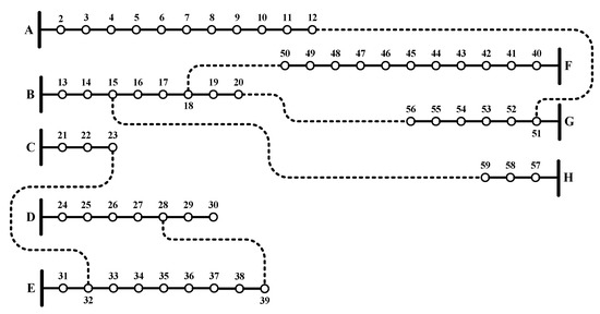
Figure 3.
Real 59-node distribution system in Cairo.
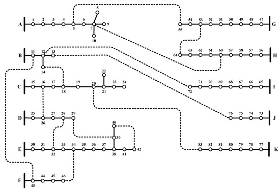
Figure 4.
Real 83-node distribution system in Taiwan.

Table 1.
Input data configurations.
4.1. Deterministic Case Study
4.1.1. Real 59-Node Distribution System in Cairo
For the 59-node distribution system, the HC reaches >98%. Table 2 provides detailed results for these three optimization techniques. Tie-lines, SOPs size, and locations are given in Table 3. The installed DG nodes and their sizes are shown in Table 4 for MOMVO.
Table 2.
Deterministic results for 59-node distribution system.
Table 3.
Tie-lines, soft open points (SOPs) size, and locations.
Table 4.
Distributed generation (DG) nodes for 59-node distribution system.
4.1.2. Real 83-Node Distribution System in Taiwan
For the 83-node distribution system, the HC reaches >98%. Table 5 gives detailed results for these three optimization techniques. It is evident that MOPSO outperformed against NSGA-II, and MOMVO by providing the best HC, and the lowest . Tie-lines, SOPs size, and locations are given in Table 6. The installed DG nodes and ratings are shown in Table 7 for MOPSO. Figure 5 shows the voltage profile improvement after allocating DGs and SOPs.
Table 5.
Deterministic hosting capacity (HC) results for 83-node distribution system.
Table 6.
Tie-lines, SOPs size, and locations.
Table 7.
DGs for 83-node distribution system.
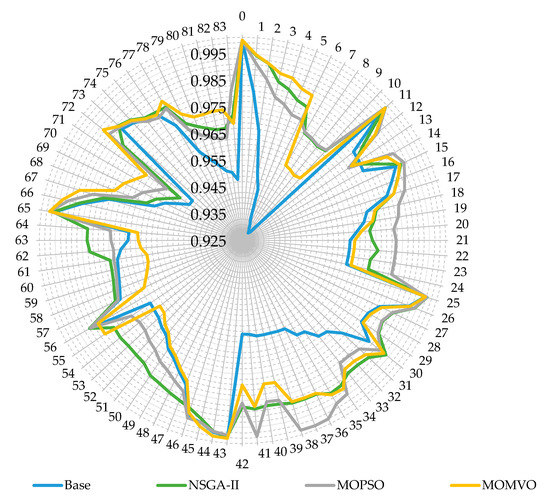
Figure 5.
Voltage profile for the 83-node system in the deterministic case.
4.2. Probabilistic Case Study
For the probabilistic case study, the uncertainty in the load over the year is considered, as shown in Figure 6. The most crucial load scenarios are generated using the scenario reduction algorithm in [31]. These scenarios are given in Table 8, including their loading levels and associated probabilities.
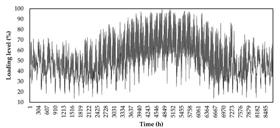
Figure 6.
Load profile over one year.
Table 8.
Load Scenarios.
4.2.1. Real 59-Node Distribution System in Cairo
For the 59-node distribution system, the HC reaches >62%, which is lower than the deterministic case study. Table 9 gives detailed results for these three optimization techniques. Tie-lines, SOPs size, and locations are given in Table 10. HCs and total power losses for the studied scenarios are shown in Figure 7 and Figure 8, respectively, and the installed DG ratings for each node are shown in Figure 9. The voltage profiles before and after allocation of DGs and SOPs for the different scenarios are shown in Figure 10.
Table 9.
Probabilistic results for the 59-node distribution system.
Table 10.
Tie-lines, SOPs size, and locations.
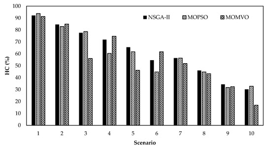
Figure 7.
HC for each scenario: 59-node distribution system.
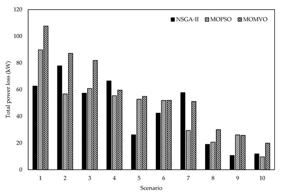
Figure 8.
Total power loss for each scenario: 59-node distribution system.
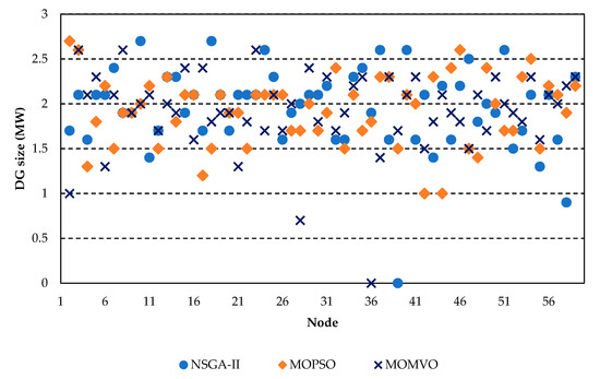
Figure 9.
DG sizes at each node: 59-node distribution system.
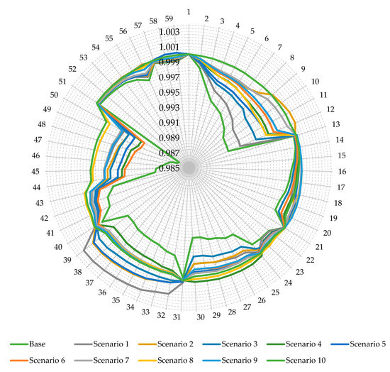
Figure 10.
Voltage profiles for the 59-node system in different scenarios.
4.2.2. 83-Node Distribution System
For the 83-node distribution system, the HC reaches >57%. Table 11 gives detailed results for these three optimization techniques. Tie-lines, SOPs size, and locations are given in Table 12. HCs and total power losses for the studied scenarios are shown in Figure 11 and Figure 12, respectively, and the installed DG ratings for each node are shown in Figure 13. The voltage profiles are shown in Figure 14 for the different scenarios before and after the allocation of DGs and SOPs. Also, the 83-node distribution network tie-lines, DGs and SOPs locations using MOPSO are shown in Figure 15.
Table 11.
Probabilistic results for the 83-node distribution system.
Table 12.
Tie-lines, SOPs size, and locations.
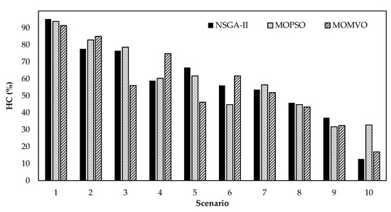
Figure 11.
HC for each scenario: 83-node distribution system.
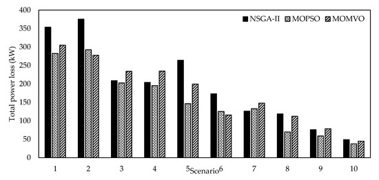
Figure 12.
Total power loss for each scenario: 83-node distribution system.
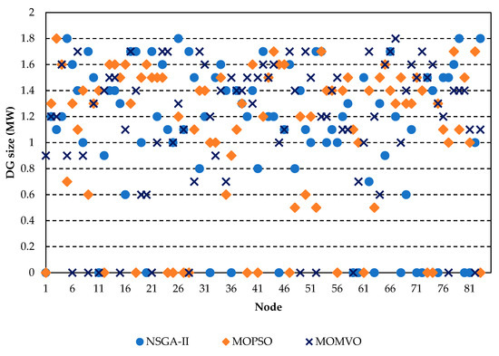
Figure 13.
DG sizes at each node: 83-node distribution system.
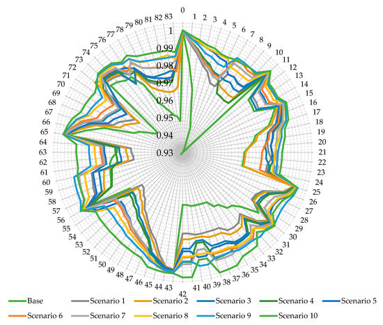
Figure 14.
Voltage profile for the 83-node system for different scenarios.
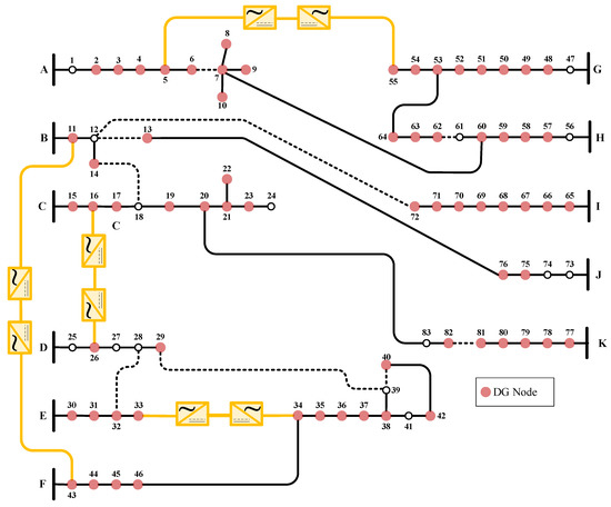
Figure 15.
83-node distribution network after SOPs and DGs allocation.
As shown in this probabilistic study, it is clear that MOPSO outperformed against NSGA-II and MOPSO in maximizing the . of the studied distribution networks up to >62%, and >60 for the 59- and the 83-node distribution systems, respectively. Thus, it is clear that the proposed DGs planning strategy has been successfully assisted via simultaneous DSR and SOPs allocation, where the 59-node distribution system accepted allocation of DGs among the distribution system nodes, and the 83-node distribution system accepted allocation of DGs among 68 nodes of the distribution network. Besides, the radiality of the non-SOP feeders is ensured, as shown in Figure 15. Also, MOPSO succeeded in maximizing the expected HC for the 59- and the 83-node distribution systems, and minimizing the expected total annual cost better than NSGA-II and MOMVO for the 83-node distribution system. Thus, in most of the study cases, MOPSO has outperformed against NSGA-II and MOPSO. To sum up, SOPs insertion, along with the reconfiguration of the non-SOP tie-lines has provided a new perspective in promoting the concept of meshed networks in the distribution grids from the planning and the economic viewpoints. Also, the proposed planning strategy was applied to real distribution feeders to step on its validity before using it on real large distribution feeders like the 415-, 880-, 1760-, and 4400-node distribution systems, which will be considered in future works.
5. Conclusions
In this work, a bilevel multi-objective optimization approach is proposed to maximize the HCs of two real distribution systems using simultaneous DSR and SOP allocation. Two case studies are conducted using both systems, including both deterministic and probabilistic optimization approaches. From the obtained results, it is clear that HC was maximized efficiently while considering the load uncertainties, and the system is expected to accommodate greater than 62% and 57% DG penetration in the 59- and 83-node distribution systems. The use of DSR with SOPs succeeded in improving the indices of the systems and also in minimizing the expected total annual costs by more than 75.5126% and 57.5967% compared to the initial annual cost for the 59- and 83-node distribution systems, respectively, at the maximum DGs penetration while considering the load uncertainties. It is therefore clear that allocating SOPs with the use of DSR succeeded in improving both the HC and the system indices. In future work, we will demonstrate the insertion of multi-terminal SOPs along with hourly DSR and energy storage system allocation for large practical distribution feeders with uncertainties.
Author Contributions
I.M.D. and S.H.E.A.A. designed the problem under study; I.M.D. performed the simulations and obtained the results. S.H.E.A.A. analyzed the obtained results. I.M.D. wrote the paper, which was further reviewed by S.H.E.A.A., A.E.-R., A.Y.A. and A.F.Z. All authors have read and agreed to the published version of the manuscript.
Funding
This research received no external funding.
Conflicts of Interest
The authors declare no conflict of interest.
Nomenclature
| Input Data | |
| Loss coefficient of each VSC | |
| Set of nodes | |
| Electricity price | |
| SOP capital cost per unit capacity | |
| Maximum line current of the bth line | |
| Total number of lines | |
| Total number of nodes | |
| Total number of tie-lines | |
| Total number of scenarios | |
| Number of the installed SOPs | |
| Demanded active power at node | |
| Probability of the sth scenario | |
| Number of years | |
| Set of all scenarios | |
| Maximum size of the installed DGs | |
| Maximum SOP size | |
| Set of tie-lines | |
| Lower voltage limit | |
| Upper voltage limit | |
| Set of lines | |
| Impedance of the bth line | |
| SOP annual operation cost coefficient | |
| Decision Variables of the DSR, the SOP size and location | |
| A binary vector indicates the best open/close status of the distribution system tie-lines | |
| A temporary binary vector indicates open/close status of the system tie-lines | |
| Binary variable allows SOP allocation instead of the yth tie-line | |
| , | VSC size at the Ith, and Jth feeders |
| Decision Variables of the Deterministic Case Study | |
| Binary variable allows DG allocation at the uth node when its value equals to one. | |
| Injected active power by the uth DG | |
| SOP active power injected at the Ith feeder | |
| SOP reactive power injected at the Ith and the Jth feeders | |
| Decision Variables of the Probabilistic Case Study | |
| Binary variable indicates DG allocation | |
| Injected active power by the uth DG | |
| SOP active power injected to the Ith feeder | |
| SOP reactive power injected to the Ith feeder | |
| SOP reactive power injected at the Jth feeder | |
References
- Shukla, A.K.; Ahmad, Z.; Sharma, M.; Dwivedi, G.; Verma, T.N.; Jain, S.; Verma, P.; Zare, A. Advances of Carbon Capture and Storage in Coal-Based Power Generating Units in an Indian Context. Energies 2020, 13, 4124. [Google Scholar] [CrossRef]
- Zsiborács, H.; Baranyai, N.H.; Vincze, A.; Zentkó, L.; Birkner, Z.; Máté, K.; Pintér, G. Intermittent Renewable Energy Sources: The Role of Energy Storage in the European Power System of 2040. Electronics 2019, 8, 729. [Google Scholar] [CrossRef]
- Zappa, W.; Junginger, M.; Broek, M.V.D. Is a 100% renewable European power system feasible by 2050? Appl. Energy 2019, 233–234, 1027–1050. [Google Scholar] [CrossRef]
- Aleem, S.A.; Hussain, S.S.; Ustun, T.S. A Review of Strategies to Increase PV Penetration Level in Smart Grids. Energies 2020, 13, 636. [Google Scholar] [CrossRef]
- Ismael, S.M.; Aleem, S.H.A.; Abdelaziz, A.Y.; Zobaa, A.F. State-of-the-art of hosting capacity in modern power systems with distributed generation. Renew. Energy 2019, 130, 1002–1020. [Google Scholar] [CrossRef]
- Fatima, S.; Püvi, V.; Lehtonen, M. Review on the PV Hosting Capacity in Distribution Networks. Energies 2020, 13, 4756. [Google Scholar] [CrossRef]
- Mulenga, E.; Bollen, M.H.J.; Etherden, N. A review of hosting capacity quantification methods for photovoltaics in low-voltage distribution grids. Int. J. Electr. Power Energy Syst. 2020, 115, 105445. [Google Scholar] [CrossRef]
- Abideen, M.Z.U.; Ellabban, O.; Al-Fagih, L. A Review of the Tools and Methods for Distribution Networks’ Hosting Capacity Calculation. Energies 2020, 13, 2758. [Google Scholar] [CrossRef]
- Pandi, V.R.; Zeineldin, H.H.; Xiao, W.; Zobaa, A.F. Optimal penetration levels for inverter-based distributed generation considering harmonic limits. Electr. Power Syst. Res. 2013, 97, 68–75. [Google Scholar] [CrossRef]
- Ismael, S.M.; Aleem, S.H.E.A.; Abdelaziz, A.Y.; Zobaa, A.F. Probabilistic Hosting Capacity Enhancement in Non-Sinusoidal Power Distribution Systems Using a Hybrid PSOGSA Optimization Algorithm. Energies 2019, 12, 1018. [Google Scholar] [CrossRef]
- Ismael, S.M.; Aleem, S.H.E.A.; Abdelaziz, A.Y.; Zobaa, A.F. Practical Considerations for Optimal Conductor Reinforcement and Hosting Capacity Enhancement in Radial Distribution Systems. IEEE Access 2018, 6, 27268–27277. [Google Scholar] [CrossRef]
- Alalamat, F. Increasing the Hosting Capacity of Radial Distribution Grids in Jordan. Bachelor’s Thesis, Uppsala University, Uppsala, Sweden, 2015. Available online: http://www.diva-portal.org/smash/record.jsf?pid=diva2%3A833570&dswid=5802 (accessed on 5 October 2020).
- Alturki, M.; Khodaei, A. Increasing Distribution Grid Hosting Capacity through Optimal Network Reconfiguration. In Proceedings of the 2018 North American Power Symposium (NAPS), Fargo, ND, USA, 9–11 September 2018; pp. 1–6. [Google Scholar]
- Falabretti, D.; Merlo, M.; Delfanti, M. Network reconfiguration and storage systems for the hosting capacity improvement. In Proceedings of the 22nd International Conference on Electricity Distribution, Stockholm, Sweden, 10–13 June 2013; pp. 10–13. [Google Scholar]
- Fu, Y.Y.; Chiang, H.D. Toward optimal multi-period network reconfiguration for increasing the hosting capacity of distribution networks. In Proceedings of the IEEE Power Energy Society General Meeting 2018, Portland, OR, USA, 5–9 August 2018; pp. 1–5. [Google Scholar]
- Fu, Y.-Y.; Chiang, H.-D. Toward Optimal Multiperiod Network Reconfiguration for Increasing the Hosting Capacity of Distribution Networks. IEEE Trans. Power Deliv. 2018, 33, 2294–2304. [Google Scholar] [CrossRef]
- Capitanescu, F.; Ochoa, L.F.; Margossian, H.; Hatziargyriou, N.D. Assessing the Potential of Network Reconfiguration to Improve Distributed Generation Hosting Capacity in Active Distribution Systems. IEEE Trans. Power Syst. 2015, 30, 346–356. [Google Scholar] [CrossRef]
- Takenobu, Y.; Yasuda, N.; Minato, S.; Hayashi, Y. Scalable enumeration approach for maximizing hosting capacity of distributed generation. Int. J. Electr. Power Energy Syst. 2019, 105, 867–876. [Google Scholar] [CrossRef]
- Xu, X.; Li, J.; Xu, Z.; Zhao, J.; Lai, C.S. Enhancing photovoltaic hosting capacity—A stochastic approach to optimal planning of static var compensator devices in distribution networks. Appl. Energy 2019, 238, 952–962. [Google Scholar] [CrossRef]
- Divshali, P.H.; Soder, L. Improving Hosting Capacity of Rooftop PVs by Quadratic Control of an LV-Central BSS. IEEE Trans. Smart Grid 2017, 10, 919–927. [Google Scholar] [CrossRef]
- Alturki, M.; Khodaei, A.; Paaso, A.; Bahramirad, S. Optimization-based distribution grid hosting capacity calculations. Appl. Energy 2018, 219, 350–360. [Google Scholar] [CrossRef]
- Al-Saadi, H.; Zivanovic, R.; Al-Sarawi, S.F. Probabilistic Hosting Capacity for Active Distribution Networks. IEEE Trans. Ind. Inform. 2017, 13, 2519–2532. [Google Scholar] [CrossRef]
- Ji, H.; Li, P.; Wang, C.; Song, G.; Zhao, J.; Su, H.; Wu, J. A Strengthened SOCP-based Approach for Evaluating the Distributed Generation Hosting Capacity with Soft Open Points. Energy Procedia 2017, 142, 1947–1952. [Google Scholar] [CrossRef]
- Thomas, L.J.; Burchill, A.; Rogers, D.J.; Guest, M.; Jenkins, N. Assessing distribution network hosting capacity with the addition of soft open points. In Proceedings of the IET Conference Publications; IEEE: Piscataway, NJ, USA, 2016. [Google Scholar]
- Ji, H.; Wang, C.; Li, P.; Zhao, J.; Song, G.; Wu, J. Quantified flexibility evaluation of soft open points to improve distributed generator penetration in active distribution networks based on difference-of-convex programming. Appl. Energy 2018, 218, 338–348. [Google Scholar] [CrossRef]
- Mohamed Diaaeldin, I.; Abdel Aleem, S.H.E.; El-Rafei, A.; Abdelaziz, A.Y.; Zobaa, A.F. A Novel Graphically-Based Network Reconfiguration for Power Loss Minimization in Large Distribution Systems. Mathematics 2019, 7, 1182. [Google Scholar] [CrossRef]
- Bloemink, J.M.; Green, T.C. Increasing photovoltaic penetration with local energy storage and soft normally-open points. In Proceedings of the 2011 IEEE Power and Energy Society General Meeting, Detroit, MI, USA, 24–28 July 2011; pp. 1–8. [Google Scholar]
- Bloemink, J.M.; Green, T.C. Benefits of Distribution-Level Power Electronics for Supporting Distributed Generation Growth. IEEE Trans. Power Deliv. 2013, 28, 911–919. [Google Scholar] [CrossRef]
- Diaaeldin, I.M.; Aleem, S.H.E.A.; El-Rafei, A.; Abdelaziz, A.Y.; Zobaa, A.F. Optimal Network Reconfiguration in Active Distribution Networks with Soft Open Points and Distributed Generation. Energies 2019, 12, 4172. [Google Scholar] [CrossRef]
- Wang, C.; Song, G.; Li, P.; Ji, H.; Zhao, J.; Wu, J. Optimal siting and sizing of soft open points in active electrical distribution networks. Appl. Energy 2017, 189, 301–309. [Google Scholar] [CrossRef]
- Growe-Kuska, N.; Heitsch, H.; Romisch, W. Scenario reduction and scenario tree construction for power management problems. In Proceedings of the 2003 IEEE Bologna Power Tech Conference Proceedings, Bologna, Italy, 23–26 June 2003; Volume 3, pp. 152–158. [Google Scholar]
- Hwang, C.-L.; Lai, Y.-J.; Liu, T.-Y. A new approach for multiple objective decision making. Comput. Oper. Res. 1993, 20, 889–899. [Google Scholar] [CrossRef]
- Saleh, O.A.; Elshahed, M.; Elsayed, M. Enhancement of radial distribution network with distributed generation and system reconfiguration. J. Electr. Syst. 2018, 14, 36–50. [Google Scholar]
- Brownlee, A.E.I.; Wright, J.A. Constrained, mixed-integer and multi-objective optimisation of building designs by NSGA-II with fitness approximation. Appl. Soft Comput. 2015, 33, 114–126. [Google Scholar] [CrossRef]
- Zhao, X.; Jin, Y.; Ji, H.; Geng, J.; Liang, X.; Jin, R. An improved mixed-integer multi-objective particle swarm optimization and its application in antenna array design. In Proceedings of the 2013 5th IEEE International Symposium on Microwave, Antenna, Propagation and EMC Technologies for Wireless Communications, Chengdu, China, 29–31 October 2013; pp. 412–415. [Google Scholar]
- Mirjalili, S.; Jangir, P.; Mirjalili, S.Z.; Saremi, S.; Trivedi, I.N. Optimization of problems with multiple objectives using the multi-verse optimization algorithm. Knowl. Based Syst. 2017, 134, 50–71. [Google Scholar] [CrossRef]
- PCS 6000 for Large Wind Turbines: Medium Voltage, Full Power Converters Up to 9 MVA. ABB, Brochure 3BHS351272 E01 Rev. A. Available online: http://new.abb.com/docs/default-source/ewea-doc/pcs6000wind.pdf (accessed on 10 October 2020).


Publisher’s Note: MDPI stays neutral with regard to jurisdictional claims in published maps and institutional affiliations. |
© 2020 by the authors. Licensee MDPI, Basel, Switzerland. This article is an open access article distributed under the terms and conditions of the Creative Commons Attribution (CC BY) license (http://creativecommons.org/licenses/by/4.0/).