Article

On the Ventilation Performance of Low Momentum Confluent Jets Supply Device in a Classroom

1
Department of Building Engineering, Energy Systems and Sustainability Science, University of Gävle, 80176 Gävle, Sweden
2
Division of Energy Systems, Department of Management and Engineering, Linköping University, 58183 Linköping, Sweden
*
Author to whom correspondence should be addressed.
Energies 2020, 13(20), 5415; https://doi.org/10.3390/en13205415
Submission received: 8 September 2020 / Revised: 3 October 2020 / Accepted: 13 October 2020 / Published: 16 October 2020
(This article belongs to the Special Issue Sustainable Buildings: Heating, Ventilation and Air-Conditioning)

Abstract

:
The performance of three different confluent jets ventilation (CJV) supply devices was evaluated in a classroom environment concerning thermal comfort, indoor air quality (IAQ) and energy efficiency. The CJV supply devices have the acronyms: high-momentum confluent jets (HMCJ), low-momentum confluent jets (LMCJ) and low-momentum confluent jets modified by varying airflow direction (LMCJ-M). A mixing ventilation (MV) slot jet (SJ) supply device was used as a benchmark. Comparisons were made with identical set-up conditions in five cases with different supply temperatures (TS) (16–18 °C), airflow rates (2.2–6.3 ACH) and heat loads (17–47 W/m2). Performances were evaluated based on DR (draft rating), PMV (predicted mean vote), ACE (air change effectiveness) and heat removal effectiveness (HRE). The results show that CJV had higher HRE and IAQ than MV and LMCJ/LMCJ-M had higher ACE than HMCJ. The main effects of lower Ts were higher velocities, DR (HMCJ particularly) and HRE in the occupied zone as well as lower temperatures and PMV-values. HMCJ and LMCJ produce MV conditions at lower airflow rates (<4.2 ACH) and non-uniform conditions at higher airflow rates. LMCJ-M had 7% higher HRE than the other CJV supply devices and produced non-uniform conditions at lower airflow rates (<3.3 ACH). The non-uniform conditions resulted in LMCJ-M having the highest energy efficiency of all devices.

Graphical Abstract

1. Introduction

Heating, ventilation, and air conditioning (HVAC) systems account for about 50% of the total building energy use and more than 10% of total national energy use [1]. This is because conventional HVAC strategies require a high energy input to provide airflow rates and thermal conditions adequate to maintain satisfactory and habitable indoor environments. Lowering airflow rates naturally implies low energy use and is therefore less costly. However, low airflow rates per person (L/(s⋅p)) of supply air in public buildings are connected to several issues regarding health [2,3,4], cognitive abilities [4,5,6], academic performance [5,7,8,9], work and economic productivity [3,10,11]. Thus, it is important that the airflow rates are adapted to the internal ventilation load to avoid these issues. The airflow rate can be set at a constant level or at a variable level that adapts to the demand, e.g., constant air volume (CAV) or variable air volume (VAV) [12], respectively. Recent studies on the implementation of VAV in office buildings, shows that VAV has a great potential to improve the indoor air quality (IAQ) and occupant health [13], and greatly reduce the HVAC energy use [13,14], consequently reducing building operational costs [14,15,16].
Wargocki and Wyon [17] showed that pupils’ performances on four out of eight given tasks increased when the airflow rate increased from 5 to 10 L/(s⋅p). The study also reported an increase in performance when the room temperature was lowered from 25 °C to 20 °C. Other studies have shown that elevated room temperatures reduce pupils’ ability to perform typical school tasks [6,7,8,18,19,20]. A recent meta-analysis shows the same correlation for productivity and room temperature in office environments that occurs in schools, but to a lesser degree [21]. A number of studies have been performed on the application of optimizing the supply air temperature (TS) with regard to internal heat load and outdoor temperature [21,22,23]. Studies show that about 29–36% [22,23] of annual energy use could be saved by optimizing TS in relation to the heat loads in educational environments instead of maintaining a constant supply temperature. Similarly, 30–39% of the energy use could be saved in an office environment by having a varying supply temperature adapted to the internal heat load [24].
It is common practice in buildings to install a mixing ventilation (MV) system, which is designed to dilute the polluted room air with conditioned supply air to lower the contaminant concentration and regulate the room temperature [25]. The air is supplied with high momentum, mainly from the ceiling, which results in homogeneous indoor environments with good thermal comfort. However, MV systems have lower air change effectiveness (ACE) and lower heat removal effectiveness (HRE) compared to stratified systems and therefore a lower energy efficiency [26,27].
Another common ventilation principle is displacement ventilation (DV), which is a stratified system operated with low momentum air supplied below room air temperature at floor level, resulting in vertical gradients of temperature and contaminant distribution in the room [27]. DV has a high heat removal effectiveness and high air change effectiveness [26,27]. However, DV can only be effectively used in cooling mode and have some issues with thermal comfort and draft complaints [26,28].
A new stratified hybrid ventilation system, with performance between displacement ventilation and mixing ventilation, based on confluent jets (CJ) with medium momentum air supplied at floor level, has been the subject of numerous recent studies [29,30,31,32,33,34]. CJ occur when jets issued from different nozzles in the same plane and running in a parallel direction coalesce downstream and move as a single jet [27]. Several studies of the dynamics of CJ show that spacing between the jets, the nozzle diameter and the jet velocity have the highest influence on the characteristics of the CJ flow behavior [35,36,37,38]. As a result, the downstream flow pattern is highly dependent upon the CJ configuration and boundary conditions. Velocity decay of CJ are slower than a single jet at the same amount of flow rate because of better conservation of the jets’ momentum [26,27,39]. Confluent jets ventilation (CJV) has been experimentally and numerically studied in [29,30,31,32,33,34,40,41]. These studies have been carried out in different environments such as classrooms [29,33,41], offices [30,34,40] and assembly halls [32]. The studies show that CJV has higher penetration [29,32] and better thermal comfort [32,34,41] compared to DV. The reason why CJV has higher penetration than DV and higher energy efficiency than the MV is the high momentum of the supply air in the occupied zone [42]. The study presented in [43,44] that employed different integrations of CJ in ventilation systems has reported benefits on perceived indoor climate.
This study is part of an ongoing research project [31,41,45] with the aim to investigate the optimal design of an air supply device based on CJ for a classroom environment. To the authors’ knowledge, the research carried out on CJV has focused on comparing different configurations of CJV to other air distributions systems in different environments with varying boundary conditions. In order to optimize CJV for different indoor environments and boundary conditions, more knowledge and understanding are required regarding the effects of the CJ configuration and supply conditions. Therefore, four supply devices with different configurations are compared in order to investigate the perceived indoor climate when the airflow rate, supply air temperature and internal heat load are varied. The performance of the supply devices is also investigated in terms of IAQ, thermal comfort and energy efficiency.
The specific objectives of this study are to compare different configurations of CJV with each other and investigate:
  • How does the airflow rate affect thermal comfort, IAQ and energy efficiency for different types of CJV?
  • How does the supply temperature affect thermal comfort, IAQ and energy efficiency for different types of CJV?
  • How can CJV be optimized with regard to energy efficiency in a classroom environment under conditions of varying heat load, airflow rates and supply temperatures?

2. Materials and Methods

As mentioned previously, the configuration of the supply device, i.e., the nozzle spacing, nozzle diameter and jet exit velocity and its direction, are vital factors for the airflow development and distribution of the CJ in the occupied zone. It is therefore important to understand how these factors interface with airflow rate, other airflows in the room (e.g., plumes) and supply temperature, as well as how operational conditions of the supply devices influence performance.

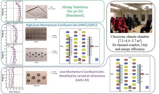
2.1. The Studied Supply Devices

In the present study, two different types of CJ supply devices with different design and characteristics are compared under the same operational conditions: internal heat load, supply airflow rates and temperatures. One of the CJ supply devices has nozzles with 28 mm in diameter, resulting in low jet exit velocity, herein referred to as low momentum confluent jets (LMCJ), and the other supply device has nozzles with 5 mm in diameter and about six times higher jet exit velocity, called high momentum confluent jets (HMCJ). A mixing slot jet (SJ) supply device is used as a benchmark during comparisons of the CJ supply devices. After analyzing results, a third CJ supply device was proposed by modifying the LMCJ with a special nozzle attachment. The modified LMCJ (LMCJ-M) was designed to increase the jet velocity (two times higher than the LMCJ) and redirect the supply air more efficiently into the occupied zone to increase the efficiency of the LMCJ based on observation from the performance of the HMCJ and LMCJ supply devices. The four studied supply devices i.e., mixing with SJ supply devices, high momentum confluent jets (HMCJ), low momentum confluent jets (LMCJ) and low momentum confluent jets modified by varying airflow direction (LMCJ-M) are shown in Figure 1. The SJ, HMCJ and LMCJ are all commonly used supply devices, which are available on the commercial market and have been obtained from commercial sources in Gävle, Sweden.

2.2. Test Facilities

The study was performed in a climate chamber (7.2 × 8.4 × 2.7 m3) at the University of Gävle in Sweden, representing a classroom environment. The climate chamber is versatile and has previously been used to investigate different indoor environments, e.g., open-plan offices [30,46], classrooms [39,44,47] and small offices [48,49].
Four mixing SJ supply devices are installed in the room, see Figure 2, and each has a rectangular outlet (0.6 × 0.6 m2) overlaid with plate to make an all-round slot of 0.02 m that issues a ceiling-attached airflow jet. All CJ supply devices were circular channels (0.25 m diameter and 4 m long) mounted 0.05 m below the ceiling level and consisted of different nozzle configurations to distinguish their classifications as HMCJ, LMCJ and LMCJ-M (refer to Figure 1), see Table 1 for specifications. The HMCJ had 576 nozzles (d = 0.005 m) at each horizontal side of the channel with a horizontal spacing of 11 jet diameters and a vertical spacing of 4 jet diameters. The LMCJ had 114 nozzles (d = 0.028 m) placed in three lines with 38 nozzles each and the middle line was slightly offset on each side of the channel, the horizontal spacing was 3 jet diameters and the vertical spacing was 1 jet diameter, see [31] for more details. The HMCJ and LMCJ directed the airflow jets in the front and back directions of the room, as shown in Figure 3 (left). The LMCJ-M is the same supply device as the LMCJ but was modified by blocking half of the nozzles on one side and re-directing airflow from some nozzles away from the outlet, as shown in Figure 3 (right). The placement of the inlets, outlet and mannequins is based on a previous field-study at a local school were the LMCJ were evaluated with varying airflow rates in a real classroom situation [41].

2.3. Equipment

Thermocouples and constant temperature anemometers (CTA) were used to measure temperatures. In total, 38 thermocouples (type K with an accuracy of ±0.2 °C) were used: 6 thermocouples were used to measure the walls, ceiling and floor temperature, 2 thermocouples measured the supply and outlet temperature and 30 thermocouples measured the vertical temperature gradient at six different locations in the occupied zone (A–F), see Figure 2. The thermocouples for the six vertical temperature gradients (VTG) were placed at heights of 0.35, 0.85, 1.4, 2.0 and 2.6 m.
CTA probes were used to measure the air speed, root mean square (RMS) of the velocity and temperature at 30 points. The probes were placed at five different heights (0.1, 0.6, 1.1, 1.7 and 2.3 m) at locations A–F. The CTA probes were calibrated for the velocity range 0.05 and 1.00 m/s and had an air speed accuracy of ±0.05 m/s and temperature sensor accuracy of ±0.2 °C. The sampling interval for all measurements was set to 60 s, with the response time of 0.2 s to 90% of a step change. In combination with the thermocouples, the temperature measurements from the CTA were used to analyze the room air temperature distribution.
Tracer gas, sulfur hexafluoride (SF6), was used to measure the local mean age of air at the locations A, B, C, D and F at a height of 1.1 m. The decay method was used to calculate the nominal time constant (τn) and the local mean age of air (τp).
Twenty-eight mannequins with a sensible heat production of about 100 W each were used to simulate the human heat load. The mannequins were designed with the same area as an average human body and consisted of a galvanized steel tube of 0.32 m diameter covered with fabric, see [50]. Other internal heat loads included heat measurement equipment, which was 50 W; no lighting load was used during the measurements. Figure 2 shows the positions of the mannequins for each heat load.

2.4. Case Set-Up

Five experimental cases were investigated, see Table 2. The cases are named after supply temperature, airflow rate per person and number of persons. Three cases had TS = 16 °C and an airflow rate of 10 L/(s⋅p), while two cases had TS = 18 °C and 15 L/(s⋅p). The difference in airflow rate between the two supply temperatures was chosen, also in relation to the heat load, to maintain the average room temperature (nominal set point = 23 °C) for all cases. The nominal set temperature was chosen to comply with a classroom with comfort category A for the winter season with corresponding clothing and activity levels according to ISO-7730 [51]. Three different heat loads were tested, as shown in Table 2: Two cases with TS = 18 °C and three cases with TS = 16 °C. The supply temperatures are set for cooling because of the heat load generated by the middle to high occupancy density in case 2, 4 and 5. The airflow rate and the size and number of nozzles affect the jet inlet velocity (U0), see Table 3.

2.5. Measurement Procedure and Analysis

Each supply device was installed and all cases measured before installing another type of supply device in the study. The experimental case was set up with each respective heat load, airflow rate and supply temperature, and the measurement equipment was left running for at least 16 h to ensure quasi-steady state conditions. The data from thermocouples and CTA probes were collected and analyzed to make sure that steady-state conditions had been reached. The last hour of the 16-h period was then used as data for each case, which were averaged and used for performance analysis. During each test, the airflow balance between the supply devices was controlled.
Trace gas measurements were done by distributing the gas throughout the room and mixing room air with movable fans (for three min) to ensure homogeneous concentration of about 400 ppm concentration. Tracer gas measurements were left running until the concentration levels had become negligible. Previous laboratory studies using the same climate chamber and measurement procedure estimate the tracer gas measurements to have an accuracy of ±7% [46,48,49].
The predicted mean vote (PMV) and percentage people dissatisfied (PPD) values were derived from the temperature measurements (thermocouples and CTA) and the air speed measurements from the CTA probes. The PMV and PPD values were calculated according to the ISO-7730 [51] and assume relative humidity RH = 35%, CLO = 0.9, and MET = 1.1 for all cases. The CLO (clothing insulation) factor and MET (metabolic equivalent of task) value correspond to winter clothing and a sedentary person performing light work i.e., typing or writing [51]. The RH was measured once during the experimental period since there is not much variation in the climate chamber. The PMV-PPD model is often complemented by the draft rating to account for the people dissatisfied by the turbulence intensity. The draft rating equation was derived experimentally by Fanger and Christensen and the model was developed with a data set where 20 < Ta < 26 °C, 0.05 < Ua < 0.5 m/s and 0 < TI < 70% [52].
The draft rating was calculated using the equation [51]:
DR = (34 − Ta) × (Ua − 0.05)0.62 × (0.37 Ua × TI + 3.14)
where Ta is air temperature, Ua is the air speed and TI is turbulence intensity. The air diffusion performance index (ADPI) was calculated using the equation [51]:
ADPI = Nθ/N
where N = total number of points and Nθ = number of points with −1.5 < θ < 1 [°K]; here, θ is defined as:
θ = (Tx − Tavg) − 7.73 × (vx − 0.15)
where Tx and vx are the temperature and velocity in each point and Tavg is average temperature in the occupied zone. The local air change effectiveness (ACEP) was calculated according to [52]:
ACEP = τnp
where τn is the nominal time constant and τp is the local mean age of air. The local heat removal effectiveness (LHRE) was calculated according to [26]:
LHRE = (TE − TS)/(TP − TS)
where TE, TS and TP are the temperature for exhaust, supply and specific measure point, respectively.
All the equations used for the thermal comfort and IAQ well defined and are commonly used within the field as measurement standards [26,27,51,52]. The absolute and RMS values of the air speed and temperature measurements are within the defined range of the measurement standard according to ISO-7750 [51] and ASHRAE [52]. The location and height of the measurement points are all according to the same standards. The CTA probes’ calibration range (0.05–1.00 m/s), accuracy (±0.05 m/s, ±0.2 °C) and response time (0.2 s to 90% step change) are sufficient to evaluate the PMV-PPD, ADPI and DR values according to both the ISO-7750 and ASHRAE standards.

3. Results and Discussion

3.1. Comparison of the SJ, HMCJ and LMCJ Supply Devices

This section presents general finding on thermal comfort, IAQ, uniformity of air distribution and energy efficiency for each supply device when the supply temperature and airflow rate is changed. The focus is on the trends for each supply device and seeing how sensitive they are to variations of supply temperature and airflow rate, but not on making a direct case by case comparison between the supply devices. Because of the differences between the different supply devices (such as ducts’ pressure drop and positions), there is some variation in the boundary conditions for each measured case compared to the nominal case setup. The differences are in airflow, supply temperature and jet inlet velocity (U0), see Appendix A Table A1. These differences in the airflow and supply temperature are rather low and should not interfere any analysis of the general trends for each individual supply device regarding the IAQ, thermal comfort and energy efficiency under variation of velocity and supply temperature. However, in Case 4 the SJ differs from the nominal case in the opposite direction from the two CJ supply devices, both for the supply temperature and the airflow. Hence, in Case 4, the SJ has −0.2 °C and +4% (0.4 L/(s⋅p), the HMCJ has +0.2 °C and −2% (0.2 L/(s⋅p)), and the LMCJ has +0.1 °C and −6% (−0.4 L/(s⋅p)). This makes it difficult to compare SJ supply device with the two CJ supply devices for this case in terms of temperature, PMV and ADPI. The CJ supply devices for example have higher Tavg and higher PMV then SJ in this case, even though they consistently have a much higher LHRE than SJ for all cases. The results regarding temperature, PMV and ADPI for this case are discussed in the next section.

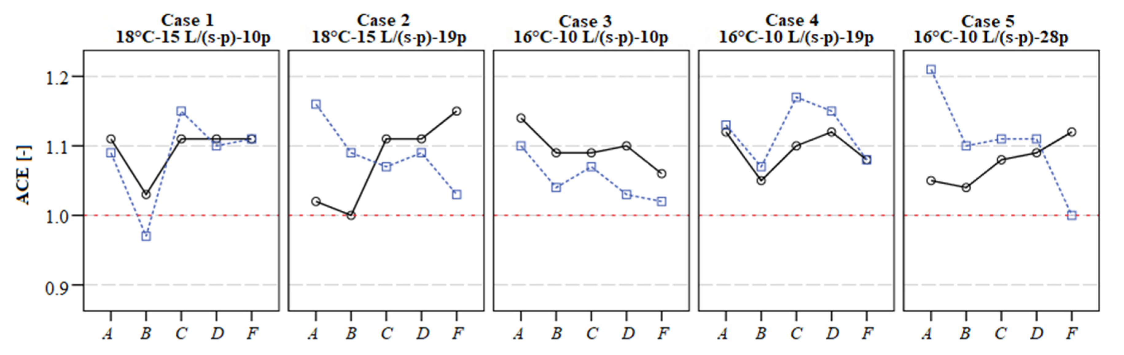
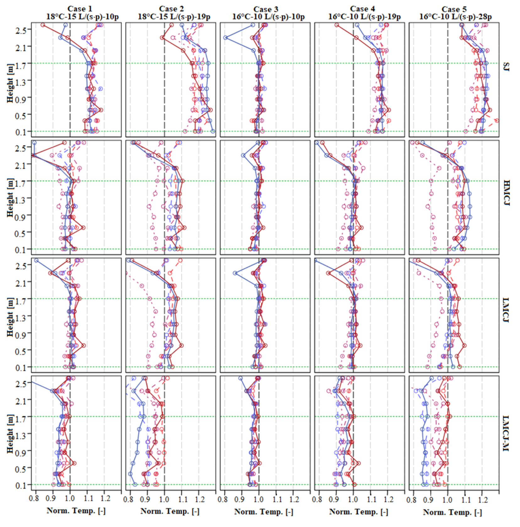
3.1.1. Air Flow Distribution and Its Effects on Temperature and Energy Efficiency

Figure 4 shows that the SJ supply device has the lowest velocities and HMCJ have the highest velocities. In the low airflow rate Cases 1 and 3, all three supply devices have more or less the same velocity profiles with very homogeneous conditions. This indicates that the two CJ supply devices as well as the SJ supply device act as MV in Case 1 and 3. In Case 4 where the airflow rate is raised, the HMCJ and LMCJ starts to behave more as a CJV system with less homogeneous conditions. In the high airflow Cases 2 and 5, both HMCJ and LMCJ have become fully CJV systems with unique velocity profiles, whilst SJ still acts like a MV system with homogenous conditions and only slightly higher velocities close to the floor in point F. The difference in nozzle configuration between HMCJ and LMCJ results in different velocity conditions in the room in the high airflow case. This is due to the CJ effects where the air follows the ceiling and walls and enter the occupied zone via the floor. HMCJ has high velocities at all heights in point D; this is most likely because this is where the CJs from both supply devices meet and are forced down into the occupied zone. LMCJ has lower velocities than HMCJ because of lower the jet inlet velocities, but it still maintains higher momentum than SJ at floor level in the high airflow rate cases, mainly in the points close to the front of the classroom (points DF) where the occupancy density is lower. Case 2 and 5 has comparable airflow rates and Tavg for the CJ supply devices but differs in supply temperature and occupancy density. For the CJ supply devices, the lower supply temperature in Case 5 compared to Case 2 seems to be the cause of higher velocities close to the floor in some of the points close to walls (A, D and F). The effects of lower supply temperature on floor level velocities is much stronger for HMCJ than LMCJ (compare Case 2 and 5).
The velocity profiles for each supply device determine the local heat removal effectiveness (LHRE). The LHRE profiles in Figure 5 are very similar to the velocity profiles in Figure 4, only less pronounced. This is supported by the fact that LHRE is related to the power three of the velocity in the occupied zone [44]. Since the SJ has the lowest velocities, it also has the lowest LHRE, which decreases as the occupancy density increases. This is because the velocities increase very little, but the heat load increases linearly with the occupancy density. The SJs LHRE profiles still have a correlation to its velocity profiles although it is very weak. Both CJ supply devices have very homogenous LHRE profiles like SJ in the cases with lower and middle airflow rates, i.e., Case 1, 3 and 4. However, in the two cases with the high airflow rates, i.e., Case 2 and 5, the LHRE becomes more diversified and adopts the behavior of the velocity profiles, which again indicate more stratified conditions than a MV system. The difference in the supply temperature and occupancy density between Case 2 and 5 does not affect the rate of LHRE for the two CJ supply devices and instead LHRE profiles follow the velocity profiles. However, the average LHRE drops 5% for the HMCJ from 101% in Case 1, 3 and 4 to 95–96% in Case 5 and 2 when the airflow rate is increased, see Table 4. Whilst the average LHRE remains stable at 99–100% for all five cases for the LMCJ. This could be due to the LMCJ’s more even velocity profiles.
As one can expect, the temperature profiles in Figure 6 are the inverse of the LHRE. All supply devices have small vertical temperature gradients (VTG) <0.8 °C. Which are quite small in terms of thermal comfort, although LMCJ have slightly higher VTG than HMCJ and SJ in the high airflow Cases 2 and 5, which indicates slightly more stratified conditions and more of a hybrid system than a MV system. The SJ has very homogenous temperature conditions for all five cases and the Tavg is highly dependent upon the occupancy density. For all three supply devices, the Tavg increases by 0.4 °C for TS = 16 °C cases when the occupancy density is raised from 10 p to 19 p. For Case 5, which has highest occupancy density, the Tavg increases for the SJ (+0.7 °C) because of lower LHRE, but the Tavg drops by 0.3–0.4 °C for HMCJ and LMCJ because of the higher velocities in the occupied zone, mostly in points close to the front of the room (DF).
There are some similarities between LHRE and ACEP, compare Figure 5 and Figure 7. SJ both have the lowest LHRE and lowest ACEP although there is more variation between points (AD and F) for ACEP than for the LHRE. HMCJ and LMCJ have comparable ACEP for the three cases with 16 °C supply temperature, with a slightly higher ACEP for the LMCJ. HMCJ performs worse when the supply temperature is raised to 18 °C compared to LMCJ but still has a higher average ACEP than SJ. LMCJ is somewhere between a DV system and a MV system, hence LMCJ acts like a hybrid system in terms of ACEP, whereas the HMJC is closer to a MV system, possibly due to higher mixing occurring because of higher nozzle-distance-to-diameter-ratio.

3.1.2. Airflow Distribution and Its Effects on Thermal Comfort

Table 4 indicates that all three supply devices have high ADPI (88–100%); this is because they all have fairly small VTG and relatively low velocities. They all perform slightly better with higher supply temperature (TS = 18 °C). They all have slightly higher ADPI when the heat load and the airflow rate is increased (compare Cases 3, 4 and 5). There is not much difference between the three supply devices, but the SJ have slightly higher ADPI than the two CJV supply devices, especially in Case 4. This is because of its more homogenous MV conditions.
The draft rate in Figure 8 shows that the SJ has the lowest and most consistent DR of the three supply devices. There is a slight increase in DR when the airflow is increased because of slightly higher velocities. However, the increase in DR is diminished because of the room temperature increase due to higher heat loads and lower LHRE. HMCJ has the highest DR and is above the recommended level in the two cases with high airflow rates (Cases 2 and 5). The supply temperature also seems to have a high influence on the DR for the HMCJ when one compares the two high airflow cases (2 and 5). Compared to the other two supply devices, the HMCJ is the only one that has points in the middle heights of the occupied zone (0.6 and 1.1 m) with DR above 20%. This is because of the higher velocities in these points resulting from higher jet velocities and the fact that the jets from the two supply devices meet in the middle of the room and push air into the occupied zone from above. The LMCJ has very similar average DR to the SJ except at point F where the DR increases more than the other points when the airflow is increased to 280–285 L/s. The DR at 0.1 m at points DE is also slightly higher than the SJ in the high airflow cases. It has only one point above 20% and that is 0.1 m at point F. The DR for LMCJ is increased by the lower supply temperature but not as much as HMCJ for the two high airflow cases. The TI for all supply devices are very similar with min/max of 20/80% and all cases have average TI of 35–41%. The max points of TI do not correspond to the max points of DR in any of the cases. One can observe variation of temperature but the variation of velocities are higher, see for example point D for HMCJ in Figure 4 and Figure 6. The variation of DR therefore is mainly due to the variation of velocity and not because of variation of temperature and TI.
Figure 9 shows the thermal comfort for a standing and seated person in all three supply devices. All three supply devices can be classified as Class B (ISO-7730), i.e., −0.5 < PMV < 0.5. The SJ supply device has the smallest variation of PMV in each case; however, it has the highest increase in PMV when the heat load is increased because of higher temperature and low velocities. The HMCJ has the highest variation of PMV mainly because of the high velocities and low temperatures at points D and F. The LMCJ has slightly higher variation of PMV than the SJ but lower than the HMCJ. The LMCJ is the only one that qualifies as Class A in the high heat load case (28 p). Both CJ supply devices have slightly higher PMV values than the SJ in the Case 4. This could be because of the variation in boundary conditions (see Appendix A Table A1) rather than low LHRE and low velocities (since the SJ is lower in both than the CJV supply devices).
The results show that if different CJ supply devices are mounted in the same position and use the same airflow and supply temperature, the configuration of the nozzles will have a great impact on the velocities in the occupied zone, which results in differing energy efficiency, air quality and thermal comfort. All three supply devices performed well in terms of ADPI, PMV and VTG. However, they all had some points with velocities and DR above recommended values. The LMCJ and HMCJ were comparable in terms of VTG, LHRE and ADPI, although the LHRE decreased by 5% for the high airflow cases for the HMCJ but not for the LMCJ. The LMCJ had better values than the HMCJ in terms of PMV and ACE (5% higher ACE on average). The results also indicate that the airflow rate determines whether the CJ supply devices produce CJV with stratified conditions or MV with homogenous conditions. Both the LMCJ and HMCJ produce homogenous conditions at an airflow rate of 2.2 to 3.3 ACH. They begin to produce more stratified conditions at an airflow rate of 4.2 ACH, and both produce full CJV at an airflow rate of 6.2 to 6.3 ACH.

3.2. The Modified Low Momentum Confluent Jets

During the comparison between the SJ, HMCJ and LMCJ, it was noticed that the velocities had a high influence on the LHRE, and HMCJ and LMCJ had high velocities in front of the room where the occupancy density is low and lower velocities in areas with higher occupancy density. This resulted in uneven LHRE and therefore variations in temperature and thermal comfort, especially for HMCJ. The LMCJ has the option to be fitted an attachment (Figure 3 bottom left) that redirects the air from the supply device. The LMCJ was modified with the attachments to redirect the air into the left side of the room in order to utilize the left wall as well as the front and back wall to direct the air into the occupied zone. Half of the nozzles facing the front side of the room were blocked. The blocking of the nozzles and the added attachments doubled the jet velocities because of the reduction in the number of nozzles and jet sizes. These changes were made in order to increase the air movement in the high occupancy area, in order to increase and balance the LHRE. The outlet was moved from the front right corner of the room to the right center side in order extract air from an area with higher occupancy density and to avoid short-circuiting. The same five cases were tested again with the LMCJ-M. The boundary conditions are presented in Appendix A Table A2. The differences between the cases are rather low and should not interfere with any analysis of the general trends, although, in Case 4, the two supply devices differ from the nominal case in opposite directions for both supply temperature and airflow. This might increase the PMV and temperature values for LMCJ slightly compared to LMCJ-M in this case.

3.2.1. The Modified Low Momentum Confluent Jets

The velocity profiles in Figure 10 are very similar for both supply devices in the low airflow Cases 1, 3 and 4. This is because they both produce relatively homogenous conditions, although, in Case 4, both of them start to produce slightly higher velocities at floor level in point F. The two high airflow Cases 2 and 5 produce stratified CJV conditions with higher airflows at floor level and lower velocities higher up. LMCJ have more stratified conditions in the front of the room, whereas because of the new configurations of the nozzles, the LMCJ-M produces more stratified conditions on the left side and in the middle of the room where the occupancy density is higher (Points: A, C and D). The lower supply temperature in Case 5 compared to Case 2 seems to increase the difference in velocities between the ankle and neck level in the room (0.1 m and 1.7 m) for LMCJ-M.
The modification of the LMCJ increases the HRE by about 3–10% depending on the airflow, see Table 5. LMCJ has a constant HRE with regard to the airflow, whereas LMCJ-M increases in LHRE as the airflow is increased. The LHRE is connected to the local velocities. LMCJ-M has higher LHRE on the left side (almost 120% for point A and C for the Case 5, see Figure 10) than on the right side (100% for B and D for the Case 5, see Figure 10), and the difference increases as the airflow is increased. In Case 3 (2.2 ACH), LMCJ-M still produces homogenous MV conditions, but, in Case 1, (3.3 ACH) starts to produce slightly more stratified conditions with higher LHRE than LMCJ and HMCJ. This is probably due to higher velocity at the floor level in the back and at the left side (points: A, B and C) for LMCJ-M. LMCJ and HMCJ starts to produce more of CJV in Case 4 (4.2 ACH), for LMCJ-M CJV is already fully developed with higher LHRE and lower temperatures in points A, C and F. When Cases 2 and 5 are compared, the lower supply temperatures and higher heat load seem to increase the velocities but not the LHRE for both LMCJ and LMCJ-M.
Figure 10 shows that the Case 3 has homogenous thermal conditions for both supply devices. However, when the airflow rate is increased slightly from 100 L/s to 150 L/s (2.2 to 3.3 ACH) with the same heat load, the LMCJ-M starts to produce more of a distinct temperature profile with lower temperatures on the left side where the LHRE and velocities are higher. This effect increases as the airflow rate is increased in Cases 2, 4 and 5. The VTG is lower for LMCJ-M than for LMCJ, especially in the front of the room (points D, E and F) where the difference in velocities between the floor and neck level is smaller for LMCJ-M than for LMCJ. The HRE is on average 7% higher for LMCJ-M than for LMCJ and is 10% higher in the high airflow Cases (2 and 5), see Table 5. The difference in Tavg between LMCJ-M and LMCJ for the TS = 18 °C Cases 1 and 2 is 0 and 0.3 °C, respectively, and the difference in Tavg for the TS = 16 °C Cases 3, 4 and 5 is 0.3, 1.0 and 0.5 °C, respectively. This indicates that the supply temperature has an effect on how much the difference in HRE affects the resulting room temperature, because of the higher velocities.
The new configuration does not change the ACE significantly. The average ACE is the same for both variants of the LMCJ, see Table 5. For the cases 1, 3 and 4 with lower airflow rates, the ACEP profiles are similar for both supply devices. In the two high airflow rate cases, the profile differs a bit for the two supply devices; the LMCJ-M has higher ACEP in the back of the room and lower in the front of the room, while the LMCJ has the opposite, see Figure 11. This pattern is somewhat reflective of the velocity pattern for the two supply devices in the high airflow rate cases.

3.2.2. Modified Airflow Distribution and Thermal Comfort

The modification of the LMCJ does not seem to change the thermal comfort significantly. The ADPI for LMCJ-M is very similar to LMCJ with only slight variation between the five cases, see Table 4. In terms of PMV, the LMCJ-M and LMCJ’s overall performance is about the same. The PMV values for LMCJ-M are quite similar to LMCJ for the two low air flow rate Cases 1 and 3; when the occupancy density and the airflow rate is increased, the PMV values for LMCJ-M drop compared to LMCJ, see Figure 12. This is because of the lower temperature as the LHRE is increased. The LMCJ and LMCJ-M have slightly different profiles in the two high airflow Cases 2 and 5. In Case 5, LMCJ-M point A is slightly too low to qualify as class A. In Case 4, the LMCJ is slightly too high to qualify as class A in points B and C; this could be due to the variations of boundary conditions. Both supply devices perform over all very well in PMV and ADPI. When the two high airflow cases are compared, it seems that the lower supply temperature in Case 5 compared to Case 2 is increasing the velocities and the DR for both supply devices. LMCJ-M has four points above the recommended value of 20% DR (Case 5) compared to one for LMCJ. The reason is not because of higher TI; it has TI values similar to the other supply devices. It has more to do with the higher velocities in the left side of the classroom, see Figure 12. The velocities as well as DR could be lowered and PMV values could be increased if the airflow rate was slightly reduced in the high airflow cases for LMCJ-M.

3.3. The Effects of Changing Airflow Distribution

Both LMCJ and HMCJ had higher velocities in the front of the classroom, resulting in lower temperatures. LMCJ-M has shifted the velocities from the front to the left side of the room. Figure 13 compares the change in velocity conditions and the resulting temperature distribution between LMCJ and LMCJ-M. The velocities in Figure 13 (right) show that the LMCJ has higher velocities in point F with low occupancy density and lower velocities in the rest of the room with high occupancy density. LMCJ-M, on the other hand, has higher velocities on the left side (points C and A), medium velocities in the middle of the room (points D and F) and the lowest velocities on the right side (points B and F) close to the outlet. This results in two different horizontal temperature distributions (HTD). LMCJ has low temperatures in point F and higher temperatures in the back, far away from the outlet, see Figure 13 (left). LMCJ-M has roughly 1 °C lower temperatures on the left side (points C and A) than LMCJ, about 0.5 °C lower temperatures in the middle (points B and D) and the same temperature at point E on the right side close to the outlet.
The effect of shifting the velocities has a quite a high impact on the temperature profile for the room when LMCJ-M is compared to SJ and HMCJ. Figure 14 shows the normalized VTG for all six points (AF). They are normalized according to:
T norm   = T P T S T E T S
As the figure shows, there is little difference in the occupied zone between the systems in the case with lowest airflow rate (Case 3). However, as the heat load and the airflow rate increase, the differences become more dissimilar; as the heat load increases, the horizontal temperature distribution (HTD) becomes more uneven for all systems but the VTG remains small. The SJ, LMCJ and HMCJ have HTD from front (cold) to back (warm), as illustrated in Figure 14 with filled lines (back) and an increasing number of spaced/dashed lines (front), whereas the LMCJ-M has HTD from left (cold) to right (warm) (blue to red in Figure 14). Since the exhaust is located to the right close to point E (see Figure 3) for LMCJ-M, the TE is close to the highest temperature in the room. This is the reason why all the Tnorm is below 1.0 in the occupied zone for all five cases with LMCJ-M. SJ, on the other hand, has higher Tnorm than 1.05 for all cases except the low airflow case (i.e., Case 1), which is probably due to a short-circuiting of the airflow when some of the air from the supply device follows the ceiling directly into the exhaust due to the Coanda effect at higher airflow rates.
If one compares Case 2 and Case 4, which have the same heat load but different supply temperatures and airflow rates, all supply devices have a more stratified HTD in Case 2 with higher supply temperature and higher airflow rate than in Case 4. This means by that the airflow rate is more determining of the stratification than the supply temperature. If one compares the two high airflow Cases 2 and 5, it is clear that the HTD is more stratified for HMCJ in Case 5 than Case 2. The same cannot be said for the two LMCJ supply devices, which means that they are less affected by lower supply temperatures or higher heat loads than HMCJ. The HTD for LMCJ-M becomes stratified to a larger degree at lower airflow rates than the two other CJ supply devices, which could be the reason for the higher LHRE.

4. Conclusions

The key observations from the results are:
  • LMCJ and HMCJ produces conditions similar to MV when the airflow rates are lower than 4.2 ACH and CJV conditions above 4.2 ACH. LMCJ-M start to produce CJV conditions at the lower airflow rates (3.3 ACH) than LMCJ and HMCJ.
  • The ACE values for the three CJ supply devices are independent of the airflow rates, the supply temperature and the occupancy density and the two LMCJs supply devices have on average 5% higher ACE than HMCJ.
  • Because of 7% higher LHRE, LMCJ-M had slightly lower temperatures and PMV-values than LMCJ, which indicates that LMCJ-M could provide similar conditions as LMCJ if the airflow rate was slightly lowered.
  • Lower supply temperatures are connected to higher velocities, lower PMV and higher DR in the occupied zone for the CJ supply devices. HMCJ was most affected by this, LMCJ-M less so and LMCJ least of all. The CJ supply devices are more sensitive to low supply temperatures in terms of thermal comfort if they have high jet inlet velocities.
  • LHRE can be increased with CJV if the air can be directed to areas with high occupancy density.
  • LMCJ and LMCJ-M become more energy efficient with a lower supply temperature because of the lower airflow rates while still being able to provide adequate thermal comfort.
  • LMCJ and LMCJ-M in combination with a lower supply temperature could be advantageous in terms of energy efficiency in countries with a cold climate where free cooling is available.
The main conclusions concerning the specific objectives can be summarized as:
  • The main effect from the airflow rate is that CJV starts to produce more stratified conditions at higher airflow rates (3.3–4 ACH) and thus become more efficient to heat removal.
  • The main effects of lower supply temperatures are higher velocities, DR and heat removal in the occupied zone as well as lower temperatures and PMV-values.
  • The LMCJ had higher ACE and better thermal comfort than the HMCJ, especially in the cases with higher heat loads and low supply temperatures. When the LMCJ was optimized for the local conditions, the results were more stratified conditions, which increased heat removal efficiency and lowered the room temperatures. This means that LMCJ-M can provide a better indoor climate with lower airflow rates and lower supply temperatures, which is more energy efficient.

5. Future Work

As this work shows, the configuration of CJV has a significant impact on the conditions in the occupied zone and an optimization of the configuration can be achieved. However, this study is limited to the specific conditions of the studied five test cases i.e., room set-up, heat loads, temperatures, airflow rates and the locations of supply devices. Therefore, further research is needed, preferably parametrical studies with a higher number of design variables (i.e., different types of rooms, different layouts, differences in nozzle configurations etc.) such as numerical studies on room level to investigate a more general approach for optimization schemes of CJV.

Author Contributions

Conceptualization, H.A., M.C. and B.M.; methodology H.A., M.C. and B.M.; formal analysis, H.A., A.K., M.C. and B.M.; investigation, H.A. and A.K.; data curation, H.A.; writing—original draft preparation, H.A.; writing—review and editing, H.A., A.K., M.C. and B.M.; visualization, H.A., A.K. and B.M.; supervision, M.C. and B.M.; project administration, H.A.; funding acquisition, B.M. All authors have read and agreed to the published version of the manuscript.

Funding

This research was funded by Repus Ventilation AB and the Knowledge Foundation (KK-Stiftelsen), grant number 20120273.

Acknowledgments

The authors gratefully acknowledge the support from the University of Gävle, Repus Ventilation AB and the Knowledge Foundation (KK-Stiftelsen). The authors are also thankful for the guidance from the industrial post-graduate school REESBE (Resource-Efficient Energy Systems in the Built Environment) and the assistance from the personnel at the Laboratory of Ventilation and Air Quality at the University of Gävle, Sweden.

Conflicts of Interest

The authors declare no conflict of interest. The funders had no role in the design of the study; in the collection, analyses, or interpretation of data; in the writing of the manuscript, or in the decision to publish the results.

Nomenclature

dInside diameter of nozzle (mm)
pPerson (-)
QTotal airflow (L/s)
QpAirflow per person (L/(s⋅p))
TEExhaust temperature (°C)
TPPoint temperature (°C)
TSSupply temperature (°C)
U0Jet inlet velocity (m/s)

Abbreviations

ACEAir Change Effectiveness
ACEPLocal Air Change Effectiveness
ADPIAir Diffusion Performance Index
CAVConstant Air Volume
CJConfluent Jets
CJVConfluent Jets Ventilation
DRDraft Rating
DVDisplacement Ventilation
HMCJHigh Momentum Confluent Jets
HREHeat Removal Effectiveness
HTDHorizontal Temperature Distribution
IAQIndoor Air Quality
LHRELocal Heat Removal Effectiveness
LMCJLow Momentum Confluent Jets
LMCJ-MLow Momentum Confluent Jets—Modified
MVMixing Ventilation
PMVPredicted Mean Vote
PPDPercentage People Dissatisfied
RHRelative Humidity
RMSRoot Mean Square
SJSlot Jet
TDTemperature Distribution
VAVVariable Air Volume
VTGVertical Temperature Gradient

Appendix A. Tables of Boundary Conditions

Table A1. Variations in boundary conditions (BC) between nominal value and measured value, Qp, TS and U0.
Case 1
18 °C-15 L/(s⋅p)-10 p
Case 2
18 °C-15 L/(s⋅p)-19 p
Case 3
16 °C-10 L/(s⋅p)-10 p
Case 4
16 °C-10 L/(s⋅p)-19 p
Case 5
16 °C-10 L/(s⋅p)-28 p
Supply DeviceBCMeasuredDiff.Diff. %MeasuredDiff.Diff. %MeasuredDiff.Diff. %MeasuredDiff.Diff. %MeasuredDiff.Diff. %
SJQP (L/(s⋅p))15.50.53%15.70.75%10.50.55%10.40.44%10.50.55%
TS (°C)17.9−0.1−0.6%17.7−0.3−1.7%16.30.31.9%15.8−0.2−1.3%1600.0%
U0 (m/s)0.860.033%1.650.075%0.580.035%1.100.044%1.630.085%
HMCJQP (L/(s⋅p))15.40.43%15.30.32%10.20.22%9.8−0.2−2%10.20.22%
TS (°C)1800.0%1800.0%1600.0%16.20.21.3%1600.0%
U0 (m/s)3.410.093%6.410.112%2.260.042%4.11−0.09−2%6.330.132%
LMCJQP (L/(s⋅p))14.5−0.5−3%14.7−0.3−2%9.8−0.2−2%9.6−0.4−4%9.9−0.1−1%
TS (°C)17.9−0.1−0.6%17.8−0.2−1.1%16.10.10.6%16.10.10.6%1600.0%
U0 (m/s)0.52−0.02−3%1.00−0.02−2%0.35−0.01−2%0.65−0.03−4%0.99−0.01−1%
Max–MinQP (L/(s⋅p))15.5–14.517%15.7–14.70.96%10.5–9.80.77%10.4–9.60.88%10.5–9.90.66%
TS (°C)18.0–17.90.11%18.0–17.70.32%16.3–16.00.32%16.2–15.80.43%16.0–16.000%
MaxU0 (m/s)3.410.093%6.410.112%2.26−0.04−2%4.11−0.09−2%6.3−0.13−2%
Table A2. Variations in boundary conditions (BC) between nominal value and measured value, Qp, TS and U0.
Case 1
18 °C-15 L/(s⋅p)-10 p
Case 2
18 °C-15 L/(s⋅p)-19 p
Case 3
16 °C-10 L/(s⋅p)-10 p
Case 4
16 °C-10 L/(s⋅p)-19 p
Case 5
16 °C-10 L/(s⋅p)-28 p
Supply DeviceBCMeasuredDiff.Diff. %MeasuredDiff.Diff. %MeasuredDiff.Diff. %MeasuredDiff.Diff. %MeasuredDiff.Diff. %
LMCJQP (L/(s⋅p))14.5−0.5−3%14.7−0.3−2%9.8−0.2−2%9.6−0.4−4%9.9−0.1−1%
TS (°C)17.9−0.1−0.6%17.8−0.2−1.1%16.10.10.6%16.10.10.6%1600.0%
U0 (m/s)0.52−0.02−3%1.00−0.02−2%0.35−0.01−2%0.65−0.03−4%0.99−0.01−1%
LMCJ-MQP (L/(s⋅p))14.7−0.3−2%14.6−0.4−4%9.9−0.1−1%10.30.33%9.6−0.4−7%
TS (°C)17.9−0.1−0.6%1800.0%16.10.10.6%15.8−0.2−1.3%15.7−0.3−1.9%
U0 (m/s)1.05−0.02−2%1.98−0.05−4%0.71−0.01−1%1.390.043%1.92−0.07−7%
Max–MinQP (L/(s⋅p))14.7–14.50.21%14.7–14.60.11%9.2–9.20.11%10.5–9.40.77%9.9–9.60.33%
TS (°C)17.9–17.900%18–17.80.21%16.1–16.100%16.1–15.80.32%16.0–15.70.32%
MaxU0 (m/s)0.97−0.02−2%2.02−0.05−2%0.66−0.01−1%1.430.042%2.100.073%

References

  1. Pérez-Lombard, L.; Ortiz, J.; Pout, C. A review on buildings energy consumption information. Energy Build. 2008, 40, 394–398. [Google Scholar] [CrossRef]
  2. Seppanen, O.A.; Fisk, W.J.; Mendell, M.J. Association of Ventilation Rates and CO2 Concentrations with Health and Other Responses in Commercial and Institutional Buildings. Indoor Air 1999, 9, 226–252. [Google Scholar] [CrossRef] [PubMed]
  3. Fisk, W.J.; Black, D.; Brunner, G. Changing ventilation rates in U.S. offices: Implications for health, work performance, energy, and associated economics. Build. Environ. 2012, 47, 368–372. [Google Scholar] [CrossRef] [Green Version]
  4. Carrer, P.; Wargocki, P.; Fanetti, A.; Bischof, W.; Fernandes, E.D.O.; Hartmann, T.; Kephalopoulos, S.; Palkonen, S.; Seppänen, O. What does the scientific literature tell us about the ventilation–health relationship in public and residential buildings? Build. Environ. 2015, 94, 273–286. [Google Scholar] [CrossRef]
  5. Allen, J.G.; Macnaughton, P.; Satish, U.; Santanam, S.; Vallarino, J.; Spengler, J.D. Associations of Cognitive Function Scores with Carbon Dioxide, Ventilation, and Volatile Organic Compound Exposures in Office Workers: A Controlled Exposure Study of Green and Conventional Office Environments. Environ. Health Perspect. 2016, 124, 805–812. [Google Scholar] [CrossRef] [Green Version]
  6. Kabanshi, A.; Wigö, H.; Van De Poll, M.K.; Ljung, R.; Sörqvist, P. The Influence of Heat, Air Jet Cooling and Noise on Performance in Classrooms. Int. J. Vent. 2015, 14, 321–332. [Google Scholar] [CrossRef]
  7. Bakó-Biró, Z.; Clements-Croome, D.; Kochhar, N.; Awbi, H.; Williams, M. Ventilation rates in schools and pupils’ performance. Build. Environ. 2012, 48, 215–223. [Google Scholar] [CrossRef]
  8. Wargocki, P.; Wyon, D.P. Providing better thermal and air quality conditions in school classrooms would be cost-effective. Build. Environ. 2013, 59, 581–589. [Google Scholar] [CrossRef]
  9. Norbck, D.; Nordstrm, K.; Norbäck, D.; Nordström, K. An experimental study on effects of increased ventilation flow on students perception of indoor environment in computer classrooms. Indoor Air 2008, 18, 293–300. [Google Scholar] [CrossRef]
  10. Fisk, W.J.; Rosenfeld, A.H. Estimates of Improved Productivity and Health from Better Indoor Environments. Indoor Air 1997, 7, 158–172. [Google Scholar] [CrossRef]
  11. Wyon, D.P. The effects of indoor air quality on performance and productivity. Indoor Air 2004, 14, 92–101. [Google Scholar] [CrossRef] [PubMed]
  12. Awbi, H.B. Ventilation Systems—Design and Performance, 1st ed.; Taylor and Francis: London, UK, 2008. [Google Scholar]
  13. Ben-David, T.; Rackes, A.; Waring, M.S. Alternative ventilation strategies in U.S. offices: Saving energy while enhancing work performance, reducing absenteeism, and considering outdoor pollutant exposure tradeoffs. Build. Environ. 2017, 116, 140–157. [Google Scholar] [CrossRef] [Green Version]
  14. Rackes, A.; Waring, M.S. Alternative ventilation strategies in U.S. offices: Comprehensive assessment and sensitivity analysis of energy saving potential. Build. Environ. 2017, 116, 30–44. [Google Scholar] [CrossRef] [Green Version]
  15. Hoyt, T.; Arens, E.; Zhang, H. Extending air temperature setpoints: Simulated energy savings and design considerations for new and retrofit buildings. Build. Environ. 2015, 88, 89–96. [Google Scholar] [CrossRef] [Green Version]
  16. Ben-David, T.; Rackes, A.; Lo, L.J.; Wen, J.; Waring, M.S. Optimizing ventilation: Theoretical study on increasing rates in offices to maximize occupant productivity with constrained additional energy use. Build. Environ. 2019, 166, 106314. [Google Scholar] [CrossRef]
  17. Wargocki, P.; Wyon, D.P. The Effects of Moderately Raised Classroom Temperatures and Classroom Ventilation Rate on the Performance of Schoolwork by Children (RP-1257). HVAC R Res. 2007, 13, 193–220. [Google Scholar] [CrossRef]
  18. Haverinen-Shaughnessy, U.; Shaughnessy, R.J. Effects of Classroom Ventilation Rate and Temperature on Students’ Test Scores. PLoS ONE 2015, 10, e0136165. [Google Scholar] [CrossRef] [PubMed]
  19. Wargocki, P.; Wyon, D.P. Ten questions concerning thermal and indoor air quality effects on the performance of office work and schoolwork. Build. Environ. 2017, 112, 359–366. [Google Scholar] [CrossRef] [Green Version]
  20. Porras-Salazar, J.A.; Wyon, D.P.; Piderit-Moreno, B.; Contreras-Espinoza, S.; Wargocki, P. Reducing classroom temperature in a tropical climate improved the thermal comfort and the performance of elementary school pupils. Indoor Air 2018, 28, 892–904. [Google Scholar] [CrossRef]
  21. Wargocki, P.; Porras-Salazar, J.A.; Contreras-Espinoza, S. The relationship between classroom temperature and children’s performance in school. Build. Environ. 2019, 157, 197–204. [Google Scholar] [CrossRef]
  22. Mossolly, M.; Ghali, K.; Ghaddar, N. Optimal control strategy for a multi-zone air conditioning system using a genetic algorithm. Energy 2009, 34, 58–66. [Google Scholar] [CrossRef]
  23. Parameshwaran, R.; Karunakaran, R.; Kumar, C.V.R.; Iniyan, S. Energy conservative building air conditioning system controlled and optimized using fuzzy-genetic algorithm. Energy Build. 2010, 42, 745–762. [Google Scholar] [CrossRef]
  24. Gruber, M.; Trüschel, A.; Dalenbäck, J.-O. Alternative strategies for supply air temperature control in office buildings. Energy Build. 2014, 82, 406–415. [Google Scholar] [CrossRef]
  25. Sandberg, M.; Kabanshi, A.; Wigö, H. Is building ventilation a process of diluting contaminants or delivering clean air? Indoor Built Environ. 2019, 29, 768–774. [Google Scholar] [CrossRef] [Green Version]
  26. Cao, G.; Awbi, H.; Yao, R.; Fan, Y.; Sirén, K.; Kosonen, R.; Zhang, J.J. A review of the performance of different ventilation and airflow distribution systems in buildings. Build. Environ. 2014, 73, 171–186. [Google Scholar] [CrossRef]
  27. Awbi, H.B. Ventilation of Buildings, 2nd ed.; Spon Press: London, UK, 2003. [Google Scholar] [CrossRef]
  28. Melikov, A.; Pitchurov, G.; Naydenov, K.; Langkilde, G. Field study on occupant comfort and the office thermal environment in rooms with displacement ventilation. Indoor Air 2005, 15, 205–214. [Google Scholar] [CrossRef] [PubMed]
  29. Cho, Y.; Awbi, H.; Karimipanah, T. Theoretical and experimental investigation of wall confluent jets ventilation and comparison with wall displacement ventilation. Build. Environ. 2008, 43, 1091–1100. [Google Scholar] [CrossRef]
  30. Arghand, T.; Karimipanah, T.; Awbi, H.; Cehlin, M.; Larsson, U.; Linden, E. An experimental investigation of the flow and comfort parameters for under-floor, confluent jets and mixing ventilation systems in an open-plan office. Build. Environ. 2015, 92, 48–60. [Google Scholar] [CrossRef]
  31. Andersson, H.; Cehlin, M.; Moshfegh, B. Experimental and numerical investigations of a new ventilation supply device based on confluent jets. Build. Environ. 2018, 137, 18–33. [Google Scholar] [CrossRef]
  32. O’Donohoe, P.G.; Galvez-Huerta, M.A.; Gil-López, T.; Dieguez-Elizondo, P.M.; Castejon-Navas, J. Air diffusion system design in large assembly halls. Case study of the Congress of Deputies parliament building, Madrid, Spain. Build. Environ. 2019, 164, 106311. [Google Scholar] [CrossRef]
  33. Karimipanah, T.; Awbi, H.; Sandberg, M.; Blomqvist, C. Investigation of air quality, comfort parameters and effectiveness for two floor-level air supply systems in classrooms. Build. Environ. 2007, 42, 647–655. [Google Scholar] [CrossRef]
  34. Chen, H.; Janbakhsh, S.; Larsson, U.; Moshfegh, B. Numerical investigation of ventilation performance of different air supply devices in an office environment. Build. Environ. 2015, 90, 37–50. [Google Scholar] [CrossRef]
  35. Ghahremanian, S.; Svensson, K.; Tummers, M.J.; Moshfegh, B. Near-field development of a row of round jets at low Reynolds numbers. Exp. Fluids 2014, 55, 1–18. [Google Scholar] [CrossRef]
  36. Ghahremanian, S.; Svensson, K.; Tummers, M.J.; Moshfegh, B. Near-field mixing of jets issuing from an array of round nozzles. Int. J. Heat Fluid Flow 2014, 47, 84–100. [Google Scholar] [CrossRef]
  37. Svensson, K.; Rohdin, P.; Moshfegh, B.; Tummers, M.J. Numerical and experimental investigation of the near zone flow field in an array of confluent round jets. Int. J. Heat Fluid Flow 2014, 46, 127–146. [Google Scholar] [CrossRef]
  38. Svensson, K.; Rohdin, P.; Moshfegh, B. A computational parametric study on the development of confluent round jet arrays. Eur. J. Mech. B Fluids 2015, 53, 129–147. [Google Scholar] [CrossRef]
  39. Kabanshi, A.; Wigö, H.; Sandberg, M. Experimental evaluation of an intermittent air supply system—Part 1: Thermal comfort and ventilation efficiency measurements. Build. Environ. 2016, 95, 240–250. [Google Scholar] [CrossRef]
  40. Janbakhsh, S.; Moshfegh, B. Experimental investigation of a ventilation system based on wall confluent jets. Build. Environ. 2014, 80, 18–31. [Google Scholar] [CrossRef]
  41. Andersson, H.; Cehlin, M.; Moshfegh, B. Energy-Saving Measures in a Classroom Using Low Pressure Drop Ceiling Supply Device: A Field Study. In Proceedings of the 2016 ASHRAE Winter Conference, Orlando, FL, USA, 23–27 January 2016. [Google Scholar]
  42. Nielsen, P.V. Mathematical Models for Room Air Distribution. In System Simulation in Buildings, Proceedings of the International Conference, Liége, Belgium, 6–8 December 1982, 1st ed.; Commission of the European Communities, COMAC—BME: Liége, Belgium, 1982; Volume 1, pp. 455–470. [Google Scholar]
  43. Kabanshi, A.; Wigö, H.; Ljung, R.; Sörqvist, P. Experimental evaluation of an intermittent air supply system—Part 2: Occupant perception of thermal climate. Build. Environ. 2016, 108, 99–109. [Google Scholar] [CrossRef]
  44. Kabanshi, A.; Wigö, H.; Ljung, R.; Sörqvist, P. Human perception of room temperature and intermittent air jet cooling in a classroom. Indoor Built Environ. 2016, 26, 528–537. [Google Scholar] [CrossRef]
  45. Andersson, H. Numerical and Experimental Study of Confluent Jets Supply Device with Variable Airflow. Licenciate Thesis, University of Gävle, Gävle, Sweden, 9 May 2019. [Google Scholar]
  46. Cehlin, M.; Karimipanah, T.; Larsson, U.; Ameen, A. Comparing thermal comfort and air quality performance of two active chilled beam systems in an open-plan office. J. Build. Eng. 2019, 22, 56–65. [Google Scholar] [CrossRef]
  47. Kabanshi, A.; Ameen, A.; Yang, B.; Wigö, H.; Sandberg, M. Energy Simulation and Analysis of an Intermittent Ventilation System under Two Climates. In Proceedings of the 10th International Conference on Sustainable Energy & Environmental Protection, Bled, Slovenia, 27–30 June 2017. [Google Scholar]
  48. Ameen, A.; Choonya, G.; Cehlin, M. Experimental Evaluation of the Ventilation Effectiveness of Corner Stratum Ventilation in an Office Environment. Buildings 2019, 9, 169. [Google Scholar] [CrossRef] [Green Version]
  49. Ameen, A.; Cehlin, M.; Larsson, U.; Karimipanah, T. Experimental Investigation of the Ventilation Performance of Different Air Distribution Systems in an Office Environment—Cooling Mode. Energies 2019, 12, 1354. [Google Scholar] [CrossRef] [Green Version]
  50. Mattsson, M. On the Efficiency of Displacement Ventilation, with Particular Reference to the Influence of Human Physical Activity; University of Gävle: Gävle, Sweden, 1999. [Google Scholar]
  51. ISO 7730, Moderate Thermal Environment—Determination of the PMV and PPD Indices and Specification of the Conditions for Thermal Comfort; International Organization for Standardization: Geneve, Switzerland, 2005.
  52. ASHRAE Standard 129-1997 (RA 2002)—Measuring Air Change Effectiveness; ASHRAE: Atlanta, GA, USA, 2002.
Figure 1. Photos of supply devices and nozzles, SJ, HMCJ, LMCJ, and LMCJ-M.
Energies 13 05415 g001
Figure 2. Set-up of measurement points and mannequins. (Top) Measurement points and placements of SJ and confluent jet devices, red mannequins were turned on for the 10 p (persons) cases, red and blue were turned on for 19 p cases and red, blue and yellow were turned on for the 28 p cases. (Bottom) Photo of set-up.
Energies 13 05415 g002
Figure 3. Air distribution pattern from supply devices. (Left) HMCJ and LMCJ, (Right) LMCJ-M.
Energies 13 05415 g003
Figure 4. Velocity at points AF for all cases and the supply devices @ = 0.1 m, ○ = 0.6 m, = 1.1 m, = 1.7 m and ---- = mean. Note: the mean does not represent a gradient, it is only a comparison between points.
Energies 13 05415 g004
Figure 5. Local heat removal effectiveness at Points AF for all cases and supply devices @ = 0.1 m, ○ = 0.6 m, = 1.1 m, = 1.7 m and ---- = mean. Note: the mean does not represent a gradient, it is only a comparison between points.
Energies 13 05415 g005
Figure 6. Temperature at Points AF for all cases and supply devices @ = 0.1 m, ○ = 0.6 m, = 1.1 m, = 1.7 m and ---- = mean. Note: the mean does not represent a gradient, it is only a comparison between points.
Energies 13 05415 g006
Figure 7. Air change effectiveness at Points A–D, F for all cases and supply devices @ height 1.1 m, ○ = LMCJ, = HMCJ, = SJ. Note: the lines does not represent a gradient, it is only a comparison between points.
Energies 13 05415 g007
Figure 8. Draft rating at points AF for all cases and supply devices @ = 0.1 m, ○ = 0.6 m, = 1.1 m, = 1.7 m and ---- = mean. Note: the mean does not represent a gradient, it is only a comparison between points.
Energies 13 05415 g008
Figure 9. Thermal comfort at points A–F for all cases and supply devices @ = 0.1 m, ○ = 0.6 m, = 1.1 m, = 1.7 m, ––– = Thermal comfort for standing person, ––– = Thermal comfort for seated person, - - - - = Limits for class B ISO–773, - - - - = Limits for class A ISO-7730, RH = 35%, CLO = 0.9, and MET = 1.1.
Energies 13 05415 g009
Figure 10. Velocity, LHRE and temperature at points AF for LMCJ and LMCJ-M @ = 0.1 m, ○ = 0.6 m, = 1.1 m, = 1.7 m and ---- = mean. Note: the mean does not represent a gradient, it is only a comparison between points.
Energies 13 05415 g010
Figure 11. ACE at points AD, F for LMCJ and LMCJ-M @ height 1.1 m, ○ = LMCJ, = LMCJ-M. Note: the lines does not represent a gradient, it is only a comparison between points.
Energies 13 05415 g011
Figure 12. Thermal comfort (PMV and DR) at points AF for LMCJ and LMCJ-M @ = 0.1 m, ○ = 0.6 m, = 1.1 m, = 1.7 m, –––– = thermal Comfort for standing person, –––– = thermal comfort for seated person. - - - - = limits for class B ISO–773, - - - - = limits for class A ISO-7730, RH = 35%, CLO = 0.9, and MET = 1.1. Note: the lines/mean does not represent a gradient, it is only a comparison between points.
Energies 13 05415 g012
Figure 13. Temperature (°C) (left) and velocity (m/s) (right) Case 5 at 1.1 m above the floor for LMCJ (light) A,B,C,E,D and F and the LMCJ-M (dark) A, B,C, E, D and F.
Energies 13 05415 g013
Figure 14. Normalized vertical temperature gradients for all cases. ______ = A, ______ = B, __ __ __= C, __ __ __= D, __ __ __= E, _ _ _ = F.
Energies 13 05415 g014
Table 1. Technical specifications of the supply devices.
SJHMCJLMCJLMCJ-M
Length of channel-2 × 4 m2 × 4 m2 × 4 m
Diameter of channel [m]-0.2500.2500.250
Number of Nozzles4 (slots)2 × 11522 × 228399 *
Diameter of Nozzles [m]4 × 0.6 × 0.020.0050.0280.028 **
Total Inlet Area [m2]0.180.050.280.14
Inlet Velocities [m/s]~0.6–1.6~2.2–6.3~0.4–1.0~0.7–2.0
* = The LMCJ had 465 nozzles in total, 57 of the nozzles were blocked and 228 were equipped with attachments to redirect the airflow. ** = The attachment covers half the nozzle, see Figure 1.
Table 2. Case set-up.
CasesMannequinsAirflow Rate (L/s)Heat Load (W/m2)ACH (-)
Case 1–18 °C-15 L/(s⋅p)-10 p10150173.3
Case 2–18 °C-15 L/(s⋅p)-19 p19285326.3
Case 3–16 °C-10 L/(s⋅p)-10 p10100172.2
Case 4–16 °C-10 L/(s⋅p)-19 p19190324.2
Case 5–16 °C-10 L/(s⋅p)-28 p28280476.2
Table 3. Nominal inlet velocity for all supply devices [m/s].
CasesSJHMCJLMCJLMCJ-M
Case 1–18 °C-15 L/(s⋅p)-10 p0.833.320.541.07
Case 2–18 °C-15 L/(s⋅p)-19 p1.586.301.022.03
Case 3–16 °C-10 L/(s⋅p)-10 p0.552.220.360.72
Case 4–16 °C-10 L/(s⋅p)-19 p1.064.200.681.43
Case 5–16 °C-10 L/(s⋅p)-28 p1.556.201.001.99
Table 4. Average HRE, ACE and ADPI for SJ, HMCJ and LMCJ supply devices.
Case 1Case 2Case 3Case 4Case 5Avg.
HRE
SJ89%83%100%87%87%89%
HMCJ101%96%101%101%95%99%
LMCJ99%99%100%100%99%99%
ACE
SJ95%94%98%90%93%94%
HMCJ102%98%106%107%106%104%
LMCJ109%107%110%109%108%109%
ADPI
SJ96%100%88%100%96%96%
HMCJ92%96%88%92%92%90%
LMCJ92%96%88%88%96%91%
Table 5. Average HRE, ACE and ADPI for LMCJ and LMCJ-M supply devices.
Case 1Case 2Case 3Case 4Case 5Avg.
HRE
LMCJ99%99%100%100%99%99%
LMCJ-M104%109%103%105%108%106%
ACE
LMCJ109%107%110%109%108%109%
LMCJ-M108%109%105%112%110%109%
ADPI
LMCJ92%96%88%88%96%91%
LMCJ-M88%96%88%92%92%91%
Publisher’s Note: MDPI stays neutral with regard to jurisdictional claims in published maps and institutional affiliations.

