1. Introduction
Most electricity systems worldwide are undergoing major transformations driven by the need for improving their sustainability and efficiency. These affect both their technical and economical operation and pose new challenges for all the different agents that participate in the electricity supply chain: generation, transportation, distribution and consumption. One key aspect of these transformations is the deployment of advanced metering infrastructure (AMI) technologies, which are being integrated in most electricity systems worldwide [
1]. In particular, smart meters are being progressively installed in individual households and allow tracking electricity consumption dynamics at a very disaggregated level and high frequency rates.
Moreover, since the recent deregulation of many electricity markets worldwide, there are several agents (market operators, gencos, retailers, consumers, etc.) that are highly interested on obtaining the maximum value from this type of data. In this sense, new business opportunities arise that are linked to the application and development of state-of-the-art analytics and data science techniques [
2].
Specifically, developing an accurate and computationally efficient short-term forecasting model for individual consumers (smart meters) has several important applications within the new smart grid paradigm. One of them relates to the successful implementation of demand response (DR) policies. Once real-time price tariffs are fully deployed in distribution systems, the forecasting model can learn from historical consumption patterns, as well as from each individual consumers’ reaction to prices (elasticity). This model can then be used to anticipate (forecast) the impact of different pricing strategies in both aggregated and disaggregated loads, and design these to better benefit the system. In this sense it can be helpful to identify those consumers more suitable for DR policies, anticipate and prevent systems peaks or congested lines, adapt load consumption to renewable generation availability, identify consumption anomalies that may originate from equipment failure or from electricity theft, etc.
Furthermore, smart-meter datasets may help to better understand which are the main factors that drive electricity consumption [
3], and how these can be used to improve the system’s efficiency. For instance, electricity retailers might be interested in precise load forecasts for optimal participation in futures and spot markets [
4]. Similarly, distribution companies might benefit from this sort of predictions to improve the network reliability.
For these reasons, the time series recorded by smart meters open the possibility of improving the existing forecasting models for electricity loads, from an entire system to a single household.
Until recently, most of the models proposed in the literature, and used by the industry, have focused on forecasting aggregated loads at a system or substation level. However, these models are not appropriate for dealing with time series from more disaggregated loads (buildings or individual households) [
5]. For instance, at a household level, time series are very volatile, include a high amount of noise, and are unevenly (and nonlinearly) affected by calendar effects and meteorological variables. This has motivated the used of new modeling techniques, especially in the field of Machine Learning (ML), that are able to capture potential nonlinearities among the variables, do not assume any data generation process (non-parametric), and can exploit these large datasets for their training. In particular, Artificial Neural Networks (ANN)-based models have proven effective in this type of context. One of their potential advantages, compared to traditional time series approaches, is to be able to jointly treat and combine information from several time series to improve forecasting accuracy, i.e., without studying the series in isolation [
6].
In this work we will focus on a particular ANN network architecture: Recurrent Neural Networks (RNN) with Long Short-term Memory (LSTM) [
7]. These are specifically designed to capture sequential dependencies between the data, as is the case of time series, and information from different consumers’ dynamics. However, the main drawback of these models is that to be effective, they demand a very high computational burden for their training. This may hinder their practical implementation in a smart-meter framework, as this application involves processing and forecasting up to hundreds of thousands of time series.
To overcome this difficulty, in this work we propose a new forecasting approach to deal effectively with a large number of time series, as is the case of smart-meter data. In particular, we propose to train a single LSTM-RNN model over a subset of the available smart-meter time series. We show how, after an appropriate training and parameter tuning, the resulting model can accurately predict future loads of individual consumers, even if these were not included in the original training set. Hence, the resulting tool has a great potential for large-scale applications (Big Data) as once the single network is trained, accurate individual forecast can be obtained at almost no computational cost. We test the validity of our approach under an extensive set of numerical experiments based on a real-world dataset that includes several thousand of household load time series. Results indicate that the proposed methodology can improve the forecasting accuracy of relevant benchmarks and benefit from geo-demographic segmentation of consumers in the dataset.
1.1. Literature Review
There are several works that have focused on comparing the performance of different forecasting techniques in the context of smart-meter electricity consumption data. For instance, reference [
8] compares alternative ML techniques to predict the hourly consumption loads of three residential households. A large battery of simulations suggest that the best forecasting technique depends on the particular household under study, although Least Squares Support Vector Machines shows overall good performance. A review of forecasting techniques, based on Artificial Intelligence, for electrical load demands is presented in [
9]. It shows that ANNs have a great potential, but present challenges related to initialization parameters, slow convergence or local minima. In this vein, the authors in [
10] revise several load forecasting techniques in the context of distributed energy systems. They conclude that the existing methodologies present either low forecast accuracy or high computational burden. Similar results are observed by [
11] in the contest of building electricity use prediction. In this case, the comparative study between several techniques show that the most complex one (ANN) does not necessarily leads to the highest accuracy.
With the same aim, [
12] tests the performance of several techniques (based both on classical time series and ML) to forecast individual household consumptions. Apart from considering standard predictors based on historical loads, meteorological variables and calendar effects, the authors incorporate household activity patterns, which enhance the accuracy of the predictions. Similar conclusions are obtained in [
13], where the behavior patterns are also considered to improve the predictive accuracy of individual household electricity demands. Moreover, [
14] characterizes empirically how the forecasting accuracy of different techniques varies with the level of aggregation of the series.
Other works seek to procure probabilistic forecasts for smart-meter data, in this case [
15] presents an additive quantile regression model that incorporates a boosting procedure for variable selection. The model outperforms standard probabilistic approaches for aggregated data. In a recent work and in a similar application, [
16] proposes a methodology to compute coherent probabilistic forecasts for hierarchical time series. A predictive methodology based on LASSO is proposed in [
17] to deal with sparsity and select relevant lag orders for autoregressive models. The model is applied to individual consumption data and its performance is further enhanced by including consumption series from other users.
With the recent advent of cloud and distributed computing, computationally intensive techniques such as Deep Learning (DL), and in particular RNN, have been applied to forecast disaggregated electricity loads.
With the idea of exploiting similarities between time series, [
6] proposes a forecasting framework that combines clustering and recurrent neural networks. In particular, first subgroups of time series are created based on cross-similarities and then a predictive LSTM network is trained on each subgroup. The model is tested under time series from the banking industry (monthly) and withdrawals from automatic teller machines (daily). A similar idea in the context of load forecasting is employed by [
18], where clusters of consumers with similar load patterns are formed before the adjusting a NN forecasting model for the aggregated series. A Self-Recurrent Wavelet Neural Network is used in [
19] to forecast the load of buildings in microgrids. The predictive tool makes used of feedback loops to better deal with volatile time series. Moreover, [
20] shows how an approach incorporating temporal and spatial information, can be used to identify relevant features among different households and improve the forecasting accuracy. Reference [
21] also employs a clustering analysis to extract typical daily consumption patterns that can be used to improve the accuracy of the forecasting tool.
At a district level, [
22] addresses the problem of accurate short-term load forecasting including both meteorological and technical variables. The proposed model is based on a DL algorithm that combines different back-propagation techniques to ease its computational burden. Similarly, a DL forecasting model for individual consumption time series, based on Conditional Restricted Boltzmann Machine, is presented in [
23]. The results, tested on a single consumer historical data set, show that it outperforms ANN, Support Vector Machines and RNN techniques. With the same aim, [
24] presents a pooling-based deep recurrent neural network designed to avoid overfitting. The method outperforms traditional ARIMA, Support Vector Regression and RNN. Different predictive models based on LSTM and gated recurrent unit (GRU) are proposed in [
25,
26] to provide accurate forecast for power load and air pollution time series.
An ensemble-forecasting model, that includes a LSTM network, is presented in [
27] to anticipate ultra-short-term power fluctuations and efficiently automatize power systems’ frequency control. In the same line of research, another LSTM model is further optimized in [
28] to provide accurate power fluctuations forecasts. A deep neural-network model based on LSTM architecture is used in [
29] to forecast residential loads. It is shown how, to forecast aggregated loads, in may be convenient to aggregate individual forecasts. With a similar aim and architecture, [
30] shows that the predictive accuracy can be further increased by considering appliance measurements. Another LSTM model is adapted in [
31] to provide probabilistic forecasts for household loads. To this end, a pinball loss function is used to train the model by evaluating the quantile errors.
Finally, four ML methods (including a LSTM architecture) are compared in [
32] to forecast hourly consumption of individual households. The models depend solely on historical consumption data (no external regressors). Furthermore, it is shown how the trained models exhibit certain degree of generality if tested under out-of-sample households.
1.2. Contributions
To the best of the authors’ knowledge, this is the first work that aims to develop an efficient forecasting tool for high-frequency and disaggregated loads, making an emphasis on its scalability, and hence potential application for massive (hundreds of thousand) smart-meter time series. It is worth noting that the proposed pooling-based method and RNN model share some common features with the ones proposed in [
6,
24,
32]. However, these are extended to work with high-frequency time series, to account for exogenous variables that enrich the forecasting model, and to provide accurate forecast for out-of-sample consumers and testing days.
To summarize, considering the state of the art described in the previous section, the main contributions of this work are three-fold:
To make use of a single LSTM model to produce accurate forecasts for general high-frequency time series, in our case households’ load smart meters.
To build the LSTM model so that it can be trained efficiently using only a subset of the smart meters, making it scalable and suitable to deal with massive time series (Big Data).
To validate the proposed methodology with a real-world dataset involving thousands of smart meters and by analyzing how geo-demographic segmentation can impact forecasting accuracy, and improving the out-of-sample performance over relevant benchmarks.
With these contributions, the proposed forecasting model can be efficiently trained to provide accurate near real-time forecast for hundreds of thousands of smart meters. As we show in this work, training a unique LSTM network, which is the most demanding computational task, would need to be done only once every few months, and by using just a representative subset of the smart meters time series. Once the network is trained, and its input properly defined, it can provide short-term smart meters’ forecast at almost no computational costs, as the next sections show.
1.3. Paper Organization
The rest of the manuscript is organized as follows. In
Section 2, we describe the real-world dataset and summarize the main properties of the associated time series. In
Section 3, the proposed methodology based on RNN is introduced together with the numerical results obtained in an extensive back-testing including relevant benchmarks. Finally,
Section 4 concludes by emphasizing the potential of the proposed methodology in large-scale applications.
2. Data and Descriptive Analysis
We have accessed the public energy consumption registers from [
33]. In particular, this dataset contains a sample of 5567 London households with the corresponding energy consumption, in kWh (per half hour), for each unique household identifier, date and time, and CACI ACORN categories (classification of residential neighborhoods). There are six categories that provide a geo-demographic segmentation of London’s population. Each of these six categories are further divided into a total of 18 groups, to increase homogeneity, and our methodology will be applied to each of these groups. More details about CACI ACORN classification can be found in [
34].
The proposed methodology is general and deals with high-frequency time series. Our dataset contains a frequency of half hours, but we have aggregated it into an hourly frequency to reduce a bit the dimension and the associated volatility. That means each smart meter in each of the 18 groups contains 8760 h corresponding to its energy consumption, in kWh. Please note that in any case, our methodology can also deal with half-hour data. Finally, to validate even more our methodology against the heterogeneity of the groups, we have also created another Global group with 200 smart meters randomly selected from the overall sample.
As a summary, the first row in
Table 1 contains the names of the 18 ACORN groups together with the Global Group, the second and third columns indicate the number of smart meters used by our methodology to train the LSTM model, and to test the forecasting performance, respectively. It should be noticed that no information about the meters in the test set have been used when training the model. We have considered 80% of the available meters in each group for the training set and the other 20% of the meters for the testing one. Moreover, the fourth column in
Table 1 shows the number of periods (hours) used to train the LSTM whereas the fifth column indicates the number of days the trained LSTM has been used to perform the 24-h ahead forecasts in our validation (out-of-sample test) scheme. The proposed methodology jointly treats and combines information from all the time series in a given group, hence the estimation window for the LSTM model depends not only on the number of past hours but also on the number of time series. In particular, the larger the size of the group, the smaller the number of hours needed to train the LSTM model. We have considered that the number of hours in the training set is
h over the number of meters, with a minimum of 720 h (roughly one month) and a maximum of 7200 h (roughly 10 months).
We have also removed smart meters with a high number of missing values (more than 20) and almost zero consumption (standard deviation less than 0.01 kWh). We have replaced the remaining of the missing values by the most recent real observation for each smart meter. Finally, we have also considered hourly weather data for London area in the same dates as in the smart-meter registers, as can be found in [
35].
In total, our final dataset contains hourly consumption data for 3891 smart meters (for all the 19 groups) along 2013, with a total of 8760 observations for each smart meter. In addition, our dataset also contains temperature and humidity data for each of the 8760 periods, together with extra features (calendar) as the day of the week and the hour in a day, counting a total of 33 features.
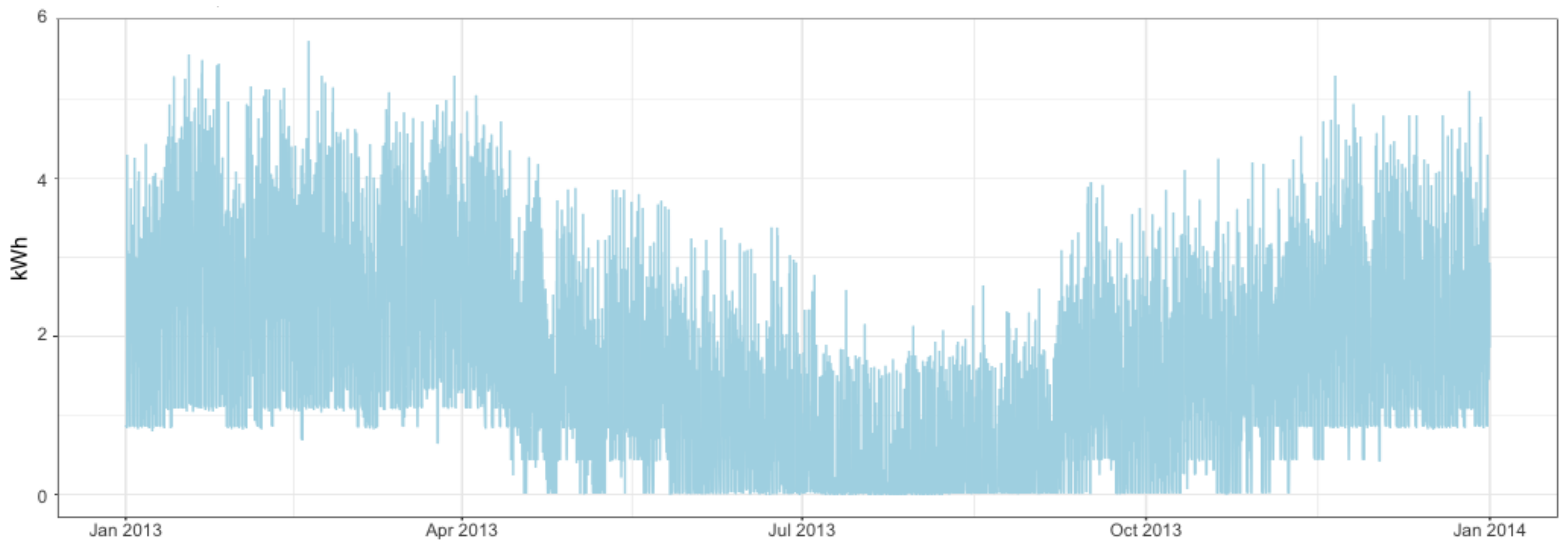
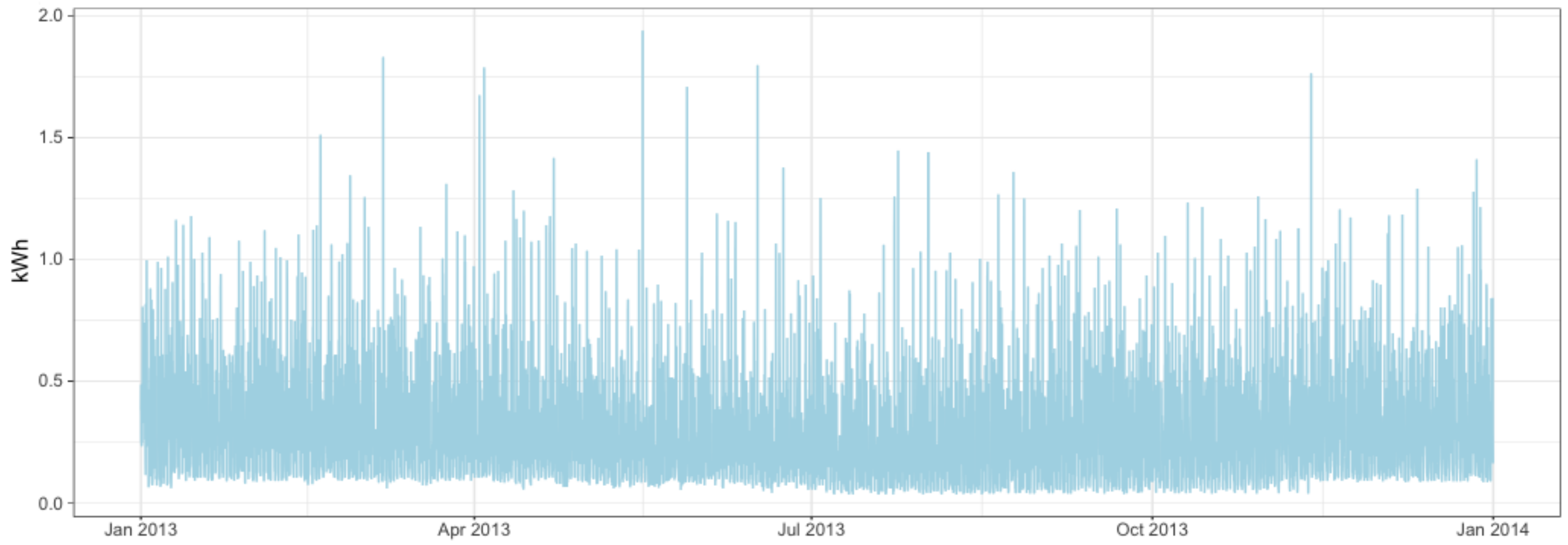
Next, a summary to understand the behavior of this dataset is provided. To have an idea, we have selected two smart meters by chance from the ACORN-A group that contains the most affluent people in the UK
lavish lifestyles. This group contains 93 households but still this group is heterogeneous. In particular, we have selected by chance the 18th and the 92nd households, and in
Figure 1 and
Figure 2 we can observe the evolution of their consumption over 2013, respectively. Note the different behavior of these two time series. Consumer 18th has a higher consumption on average with a higher volatility, but also longer periods with no consumption. On the other hand, 92nd consumer has a lower and more stable consumption, lower but strictly positive.
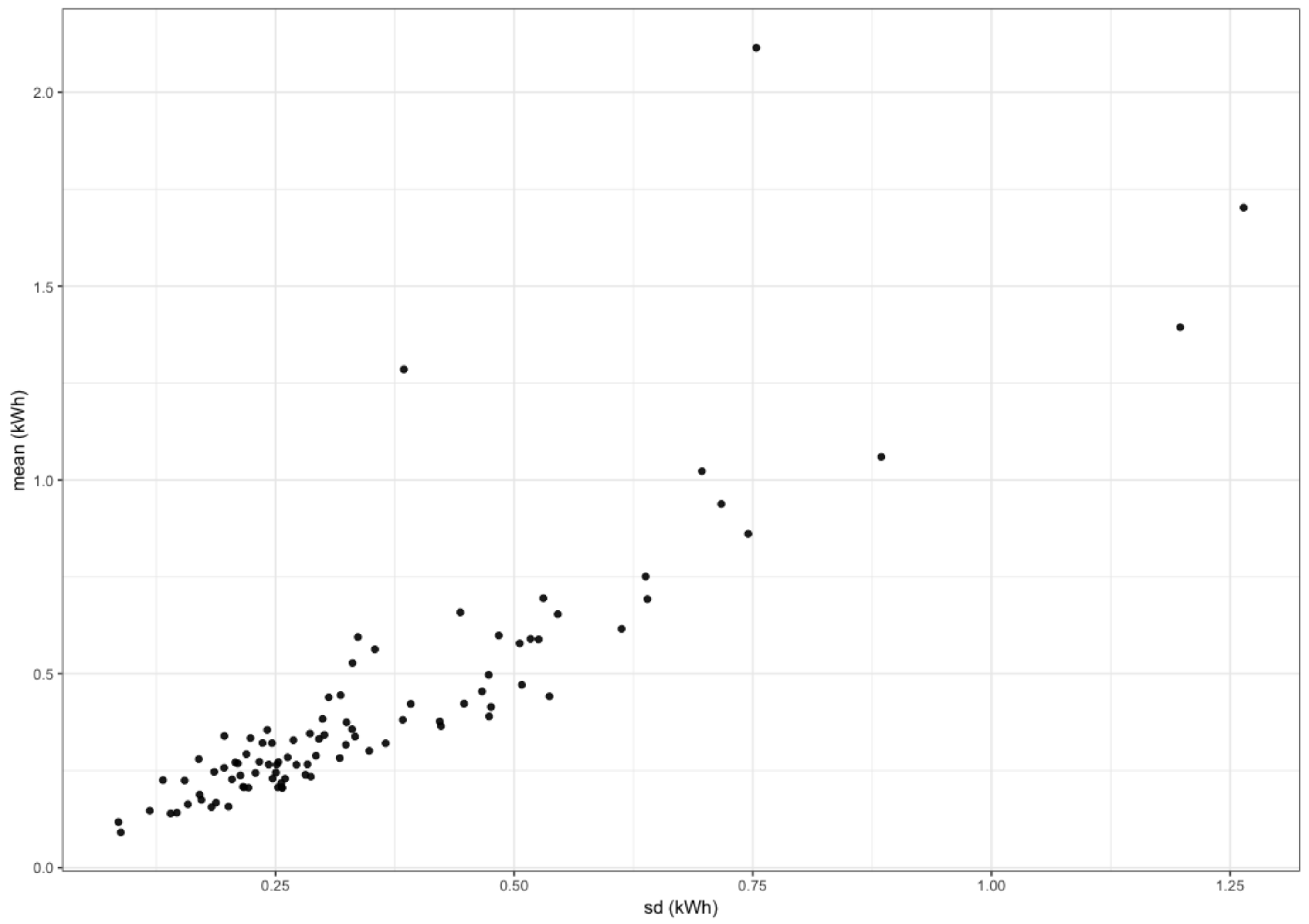
In
Figure 3, we can see a scatter plot containing the average consumption in 2013 for each smart meter in ACORN-A versus the corresponding standard deviation. Note the clear linear relationship between consumption and variability, indicating the necessity to normalize the 93 consumptions to make the group more homogeneous.
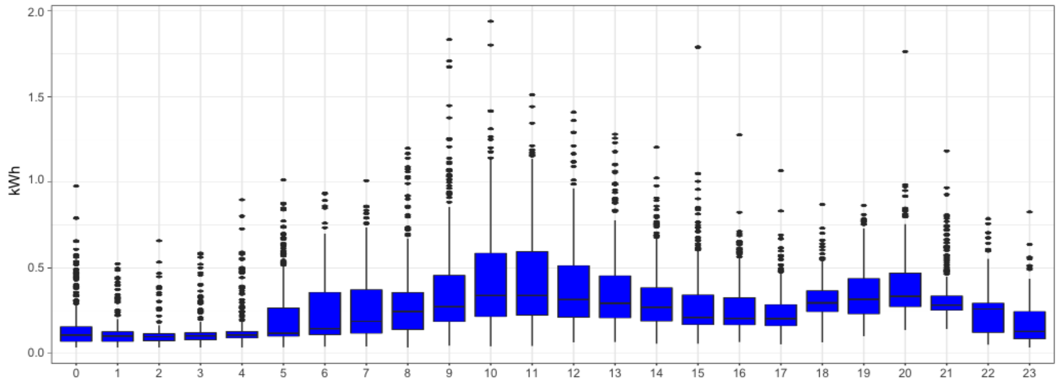
Now we will analyze the seasonality. Because we are dealing with hourly data, we expect to have several seasonalities, in particular one of order 24 (daily), other one of order 168 (weekly), and possible one of order 8760 (yearly), but the last one is not observable because we have only data for one year.
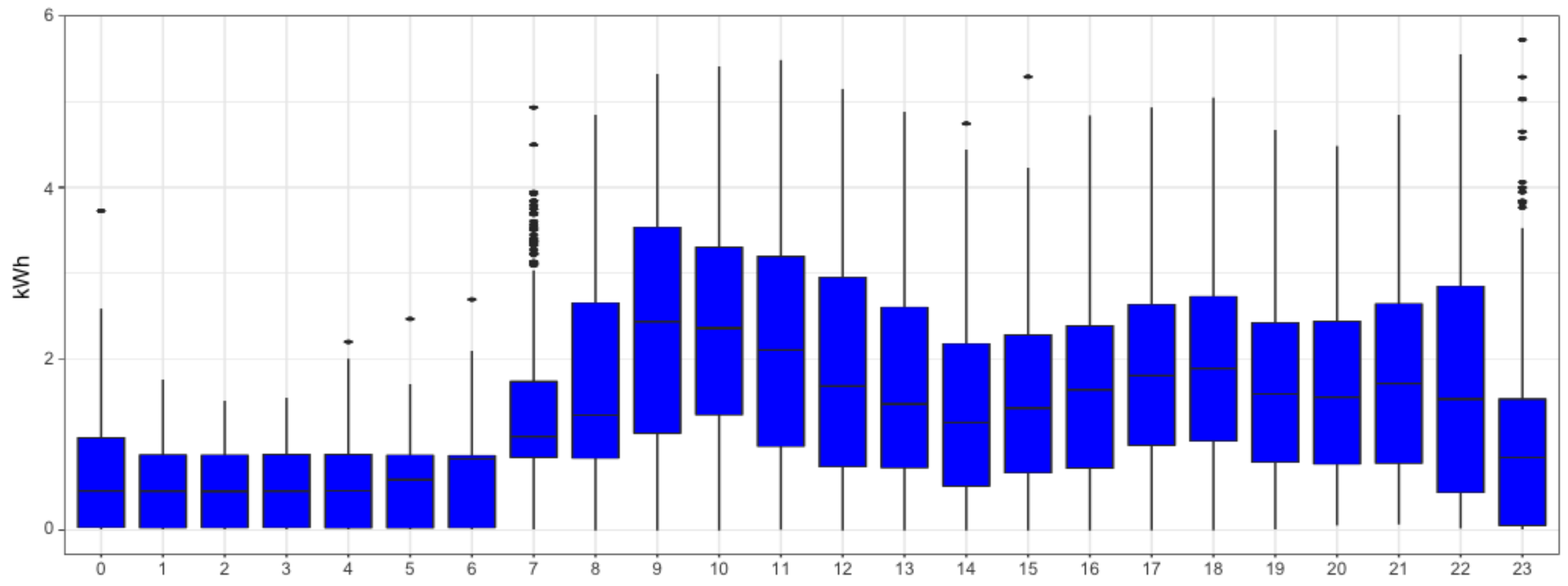
We can analyze the daily seasonality of the different smart meters. For instance,
Figure 4 and
Figure 5 reveal households that decrease consumption during night hours. A similar analysis on weekly seasonality shows that it may also play a relevant role in the time series. Hence, we will consider both the daily and weekly patterns in our methodology. Moreover, from previous figures we can also observe the asymmetric distribution of electricity consumption. This motivates our choice to apply a logarithm transformation to make it more symmetric.
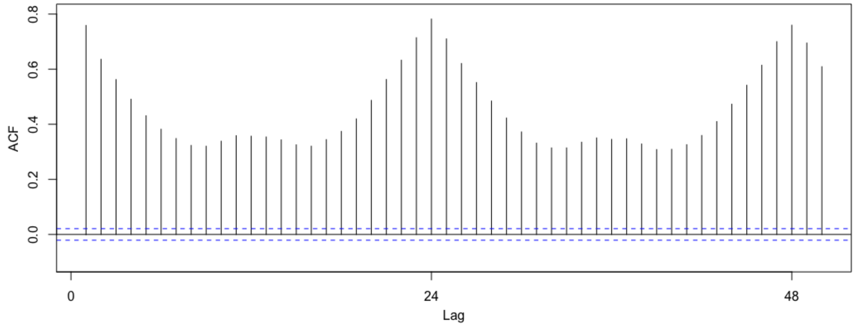
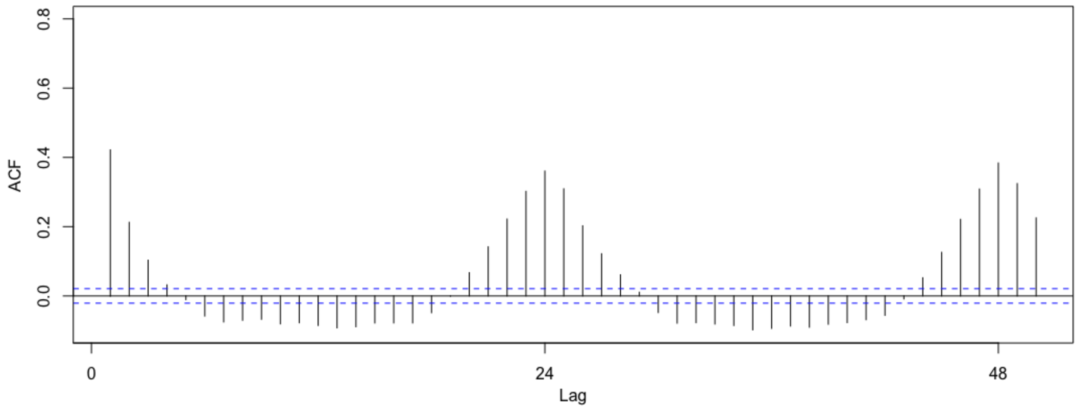
If we analyze the autocorrelations of household consumptions, useful and different patterns appear. From
Figure 6 and
Figure 7 we can observe different patterns of consumption for 18th and 92nd households, respectively. In particular, household 18th presents a high consumption dependency respect to the previous period that decays slowly (long memory). On the other hand, 92nd household presents a small dependency with a higher rate of decay (short memory). In both cases we can observe the dependency respect to previous 24 h which is an indicator of the daily seasonality previously mentioned.
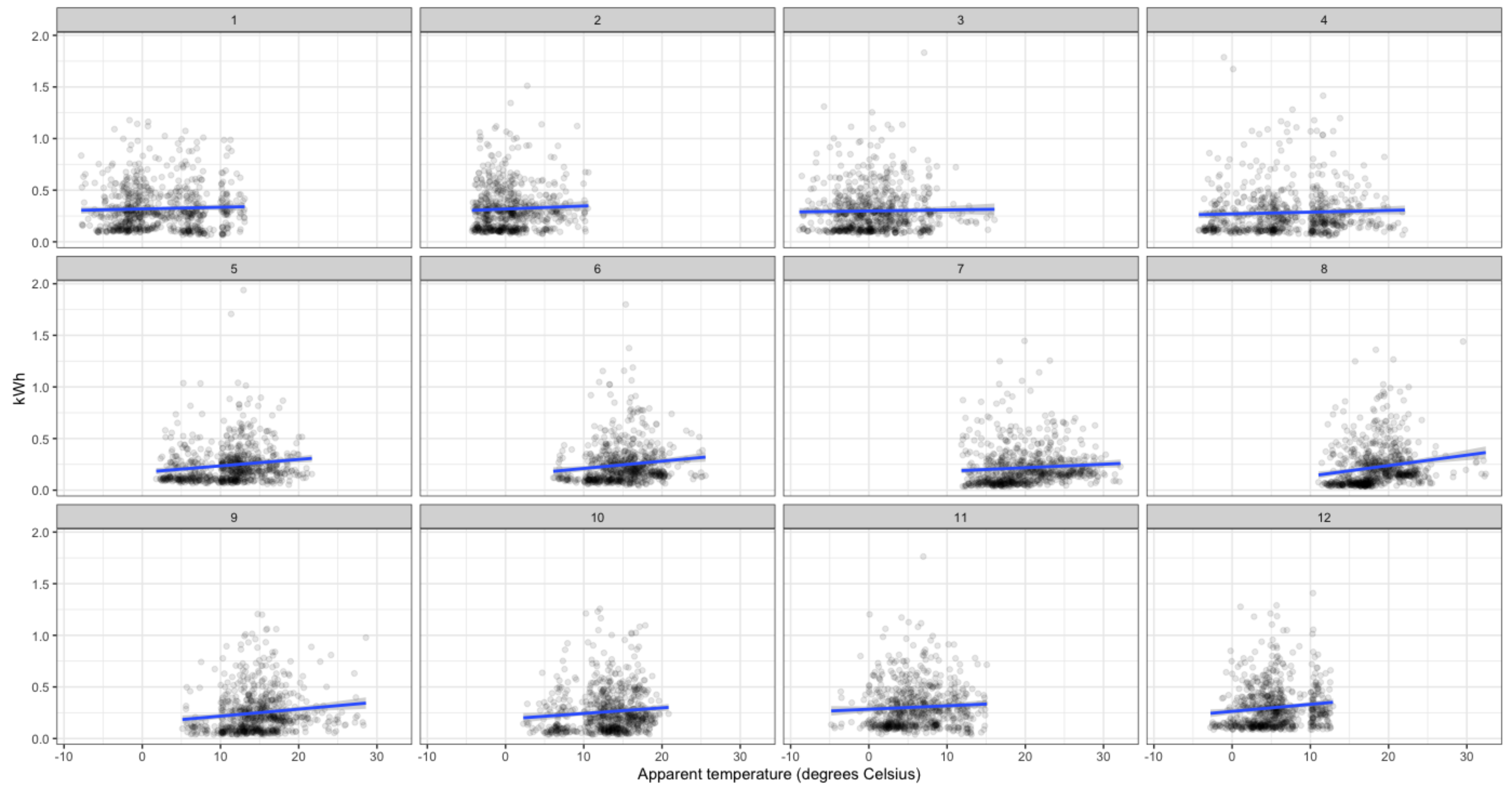
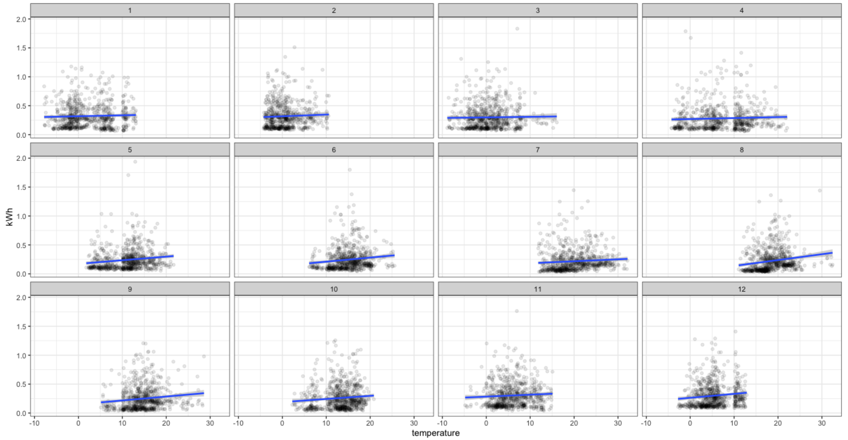
Next, we analyze the relations between the consumption and meteorological variables. For instance,
Figure 8 and
Figure 9 show the relation between consumption and temperature for the 18th and 92nd households. We can observe that this relation changes throughout the year as expected, so that it should be considered in the forecasting model. We have also repeated this analysis to other smart meters selected by chance from the other 18 groups obtaining similar insights.
As a summary of the descriptive analysis performed in this section, we have observed the collection of time series analyzed present some complex properties like high-frequency (hourly in our case), nonlinearities (especially in relations with meteorological variables), and high volatility (mainly due to the high disaggregation of the consumption). This analysis provides the inspiration and motivation for the methodology proposed in the next Section.
3. Methodology
The most difficult property to deal with this type of massive time series is the high volatility, mainly due to the underlying human behavior, which makes the relation between signal and noise unclear. One may use univariate approaches for each series, but this approach is unable to be implemented in practice (maybe millions of models to be trained/estimated) and also does not deal adequately with the non-stationarity in the data.
For this reason, we propose a methodology to deal with many time series. In particular, instead of analyzing each series in isolation, we propose to jointly treat and combine information from several time series contained in a homogeneous group. These group series may be obtained by natural grouping (in our case, the ACORN groups) or statistical clustering (for instance based on features). A review of several clustering techniques to group similar electricity consumers is presented in [
36].
Once the time series are classified into groups, a single RNN with LSTM model is trained over each group. This type of model is specifically designed to capture sequential dependencies between the data, as is the case of time series, and learn from different consumers dynamics. However, note the previous classification is not essential. Our numerical results show for the Global Group, including time series by chance, that accurate results can also be obtained without the previous clustering. However, if a previous classification of the time series into homogeneous groups is available, or a clustering of time series is performed previously to attain homogeneous groups, our methodology is able to exploit better this classification to forecast better each group.
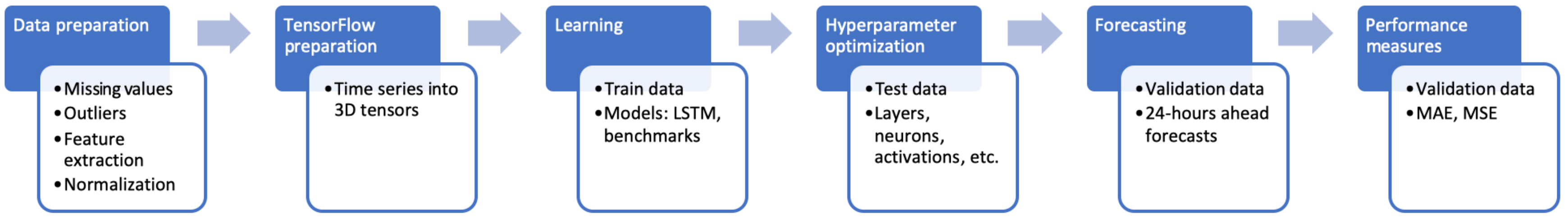
In this Section, we will explain in detail the proposed methodology, which is illustrated in
Figure 10. As mentioned before, our methodology will be based on ANN and DL because they are flexible and powerful in general, an in particular they can deal with multidimensional time series with complex interactions in a natural way. Specifically, we will use RNN for sequential data (time series) which has been proven to work successfully in natural language processing and speech recognition. Recurrent neural networks are a type of neural network where outputs from previous time steps are taken as inputs for the current time step. This creates a network graph or circuit diagram with cycles, which can be unfolded over the input sequence to make predictions over many time steps.
To train an RNN, the stochastic gradient descent is used, but gradients tend to vanish to zero too early, loosing then the available information. For this reason, LSTM networks were proposed as a type of RNN where the gradients tend to zero slower, improving then the performance.
3.1. Framework and Notation
The main and original idea of our methodology is to train one single model for all the considered time series in a given group. This is another reason to use ANN, because these models tend to perform better as the size of the input increases. Hence, we will join the information from all the time series in a group to train a LSTM model per group. Once the model has been trained using a long history, it can be used to forecast future loads not only for the smart meters considered in the training set but also for new smart meters (see
Table 1).
Next, the main notation to understand our implementation is explained. We will use the TensorFlow framework [
37] which is an open source software library for numerical computations written in C++ (and not confined exclusively to ANN). This framework was originally developed by researchers in Google to perform distributed computation, deal with large datasets, automatic differentiation, optimization algorithms, etc.
The main ingredient of the TensorFlow framework is a tensor (multidimensional matrix). As we are dealing with time series, we need a 3-dimensional framework to treat them. The first dimension is the number of samples. In our case, as we are jointly combining the information of many smart meters, the number of samples will be the number of smart meters considered in the training set times the number of periods (hours) in the training set (see second and fourth columns in
Table 1). The second dimension is the timesteps. These are separate time periods of a given variable and for a given observation with influence in future periods. As was analyzed in the previous section, it was a clear seasonality of order 24 from the daily behavior. For this reason, we have selected timesteps as 24. Finally, for the third and last dimension we need to consider the features (predictors or regressors) we have available in our dataset. In our case, we have meteorological variables (like apparent temperature and humidity), the aggregated consumption from all the smart meters in each group, 23 dummy variables for the hour of the day, and 6 dummies for the day of the week, summing up to 33 variables for the features dimension (considering also the consumption for each smart meter).
To make the implementation easier, we use Keras [
38], which is a high-level neural networks API running on top of TensorFlow. The Keras and TensorFlow frameworks allow us to implement and train the LSTM models in an easy way. In particular, we can design the network topology and estimate the weights by minimizing a differentiable loss function through the (mini-batch) gradient descent method, and compute the derivatives using back-propagation (chain’s rule). In particular, we have trained 19 LSTM models, one for each ACORN groups and the additional Global Group, with around 12,000 weights each of them that need to be estimated along a highly non-linear function from the loss function that compares the forecasts with the real values.
3.2. Data Preparation
Before applying the recurrent neural-network model, it is needed to perform some data pre-processing. This step usually needs to deal with missing values and outliers, make some feature extraction, scale and normalize the data, etc. In our case, as mentioned in
Section 2, we have replaced the missing values by the most recent observation in each smart meter. Then, we proceed to make the consumption more symmetric and take the natural logarithm as the first transformation. Later, we normalize the consumption to have the same mean and variance for all the households. These transformations are useful to make the time series more stationary, implying better performance for the LSTM model. However, we do not transform the data to remove the seasonality because the LSTM model is able to capture it in a natural way through the timesteps defined previously.
Finally, to use TensorFlow we need to convert the original input data into 3-dimensional tensors for time series. To do that, we need to build a design matrix and a target matrix. The design matrix is a tensor containing the information from the past that the LSTM will use to forecast the future. In our case, it will be a 3-dimensional array where the first dimension is
N*
T, being
N the number of smart meters and
T the number of periods considered in the past, i.e., the second and fourth columns in
Table 1. The second dimension is the timesteps, 24 in our case, denoting the number of recent observations the LSTM will be used to forecast next hours. Finally, the last dimension is the number of features, 33 in our case as explained before. The target matrix is again a 3-dimensional array where the first dimension is
N because we are interested in forecasting next period, the second dimension is the forecasting horizon for the next period, 24 in our case, and the last dimension is again 33. An example of one row of the design matrix for one smart meter would be:
where each value denotes past consumption for a given hour. An example of the same row for the target matrix and the same smart meter would be:
Note we need to build these arrays for each of the available features. Next, the details of the LSTM model will be explained.
3.3. the Proposed LSTM Model
The LSTM model in Keras is defined as a sequence of layers. In our experiments, all the LSTM models are trained with the same network topology as follows (
Figure 11). The first layer in the network defines the 3-dimensional units of the tensors as explained before. This layer is a LSTM one containing 32 units or number of neurons. Then we need to define the activation function to transform the output from each unit as the input for the next layer. The choice of this activation function is important and will affect the forecasting performance. We have used the
hyperbolic tangent as the activation function, but others can be used as the
sigmoid or
softmax ones. Then, multiple layers can be stacked by adding them to the sequential process. In our case, we have added another LSTM layer with 16 units, and finally a dense layer (or fully connected one) with 24 units that will provide the corresponding 24-h ahead forecast.
Moreover, to avoid overfitting in such a large network and improve performance, we may consider adding some type of regularization or dropout to the model. For instance, assume that we work with a group of 100 smart meters in the training set and 5000 h in each time series. Then, the number of samples is 500,000 and the number of parameters in our LSTM model is around 12,000 (with a ratio between parameters and samples of 2.4%), which makes regularization or dropout worth exploring. If we choose a regularization approach, it reduces overfitting by adding some bias to the estimation while reducing the variance. On the other hand, if we choose dropout, it reduces overfitting by randomly making zero some units in the layer during the training steps. We have chosen this last approach. In particular, the dropout rate in the network has been optimized to improve the forecasting performance, using some testing data, and considering rates from 0% to 20%. Hence, in the first recurrent layer we have selected a dropout rate of 10% of the recurrent units followed by a dropout rate of 10% for the input units of the layer. For the last LSTM layer, we have selected a dropout rate of 5%, both for the recurrent units and for the input ones.
Once we have designed the topology of the network, we need to compile it to make the estimation more efficient. To do that, we need to select the loss function and the optimization algorithm to train the network. For the loss function we have selected the mean absolute value, and for the optimization algorithm we have selected the Adam optimizer, which is a version of the stochastic gradient method, with a learning rate of .
All the previous hyper-parameters have been selected after trying other network architecture and values and observing the out-of-sample loss function. After the network is compiled for each the 19 LSTM models, we can proceed to fit or optimize the associated weights. This is the most expensive step in the methodology from a computational point of view. For this reason, we propose to train the network only once in a year, with a large number of time series and observations, and use the trained LSTM to perform the 24-h ahead forecasts for all the desired periods and smart meters in the future. This last forecasting step can be executed very fast.
The fitting or optimization process to train the network uses the back-propagation algorithm, together with the optimization algorithm and loss function defined previously. The back-propagation algorithm requires definition of the number of epochs or times the optimization algorithm uses the complete training set. In our case, we have selected 40 epochs. Each epoch can be partitioned into a fixed-sized number of rows from the training set, called batch. This subset of the training set will improve the performance of the optimization algorithm. We have selected a batch size of 1000 h (around 40 days). Once the 19 LSTM models have been trained, they are ready to perform the forecasts for all groups as the next section shows.
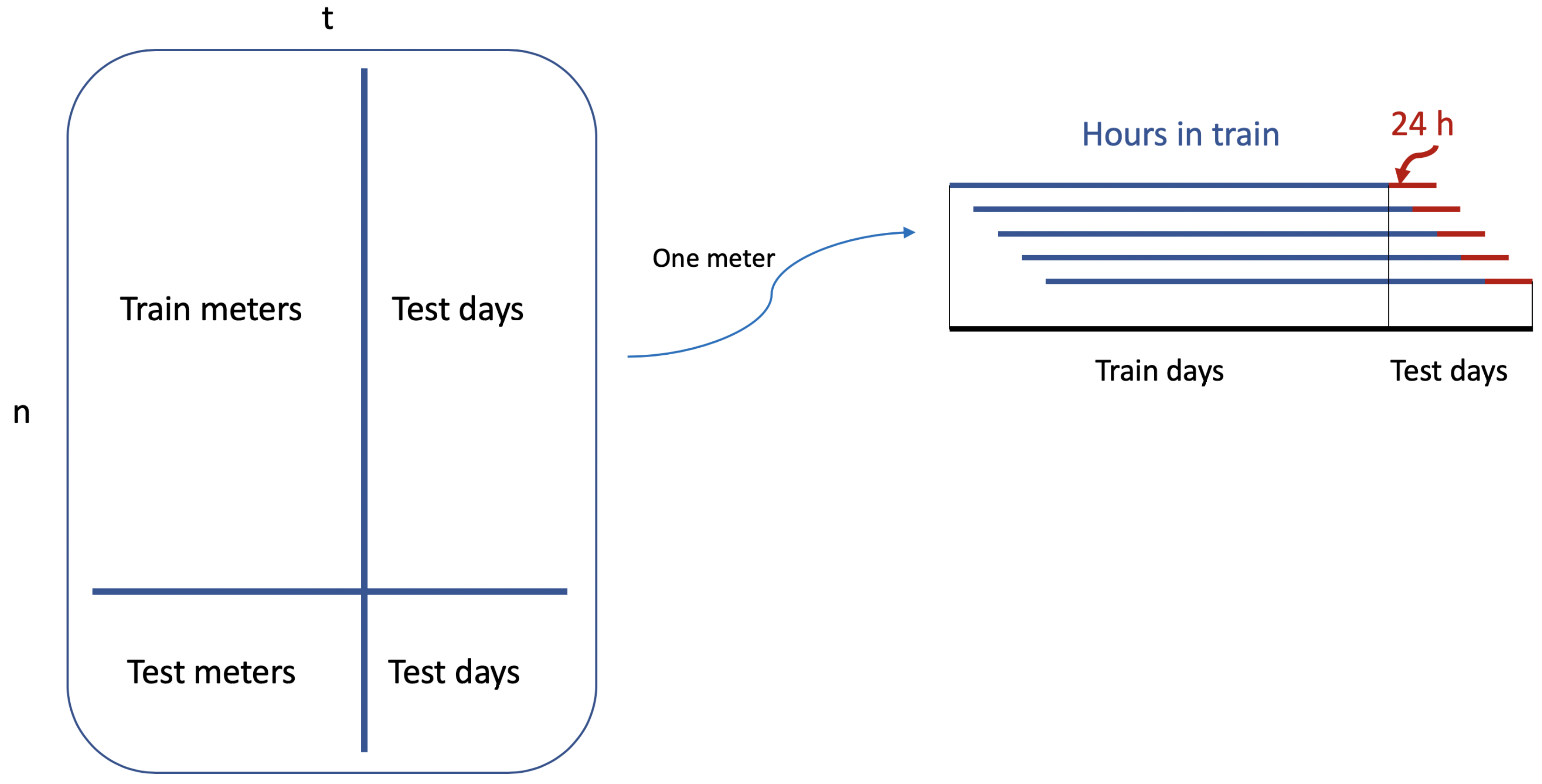
3.4. The Back-Testing
In this subsection, we explain how we have developed the back-testing scheme to evaluate the performance of the proposed methodology. First, we have information about 3891 household consumptions for all hours in 2013, i.e., 8760 h. We have organized these 3891 smart meters in 18 groups according to the ACORN classification, as summarized in
Table 1, plus the Global Group with 200 smart meters selected by chance out of the previous 18 groups. For each group, we train a LSTM (as explained in the previous section) using the number of periods indicated in the fourth column in
Table 1, leaving the last days in the sample (fifth column in
Table 1) to test the 24-h ahead forecasts for each of these days. Moreover, for each group, we have selected around 80% of the smart meters to train the models (as indicated in the second column of
Table 1), leaving the other 20% (third column in
Table 1) to test the forecasts. That means, for the out-of-sample evaluation of the models, we consider two dimensions: a time direction with out-of-sample periods, and a smart-meter direction for out-of-sample households (as they were new customers).
Besides the proposed LSTM model, we have used two well-known benchmarks: (i) a seasonal
naive approach, and (ii) an
auto.arima approach, as described in [
39]. We have also tried a
tbats method, as described in [
40], but this method becomes very unstable for some of the time series providing bad results in practice. For the seasonal
naive approach, we forecast the next 24-h ahead consumptions, with the last 24-h ones. This is one of the most successful approaches in practice, because it can be implemented and executed with little computational effort, it is stable and scalable, and provides reasonable performance for massive time series.
For the auto.arima approach, note this is an automatic framework for univariate time series. Its performance is reasonable in general, but it does not deal well with possible non-stationarity in the data and nonlinearities. Moreover, this approach is unable to implement in practice for a big energy utility because it requires the training of maybe millions of models, one for each available customer. In any case, we have implemented this approach for all the 3891 smart meters to analyze and compare better the results.
Finally, we have obtained results from our proposed LSTM model. This model requires in practice training only once or twice a year and then, individual forecasts can be obtained with little computational costs. Because we train only one model for all the time series in a group at once, our proposal has a great potential for large-scale applications.
In the next subsection, the numerical results obtained by implementing previous approaches are shown and discussed. To do that, we have computed the mean squared error (MSE) for each approach, and for each out-of-sample period and smart meter. In particular, if
denotes the real consumption of smart meter
n, for period
, and for horizon
, then the MSE for the
i-th approach,
is defined as:
for each of the out-of-sample periods
, and each of the smart meters
.
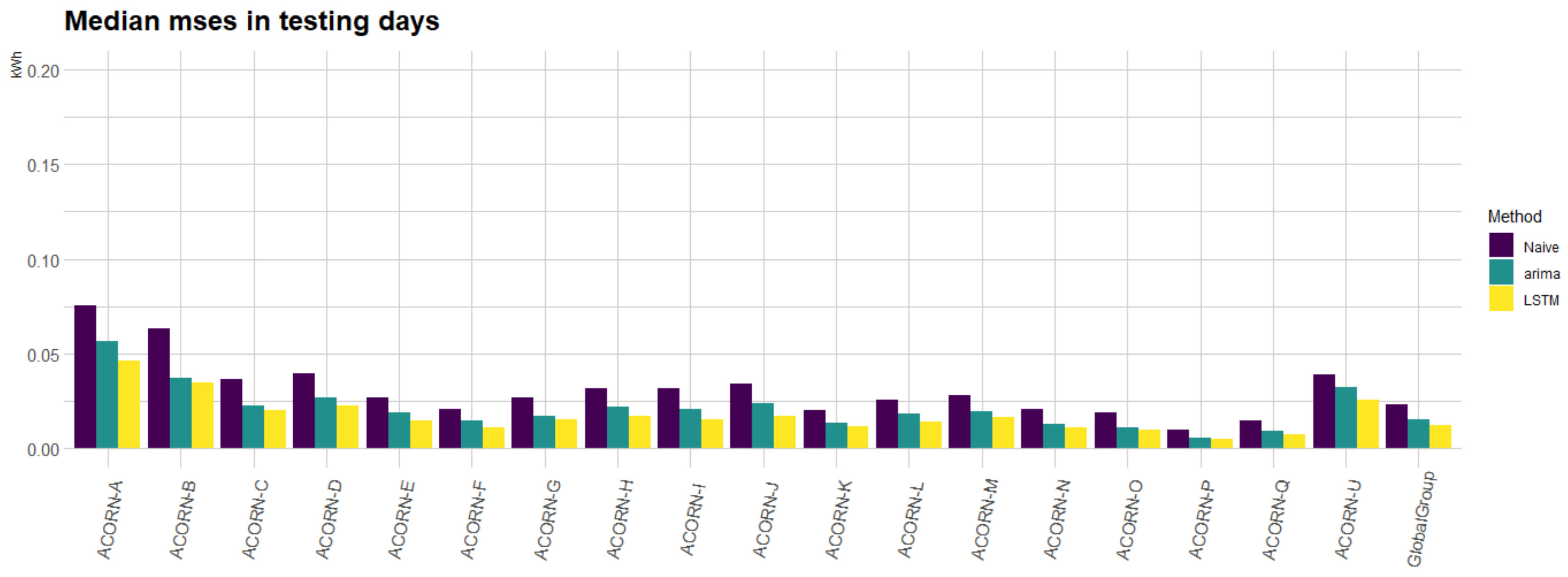
Finally, in next Subsection median MSEs are computed for each group and method: the median MSE in testing meters corresponds to the median of MSE along the out-of-sample periods
t and then the median along the testing meters
n, whereas the median MSE in testing days corresponds to the median of MSE along the meters
n and then the median along the out-of-sample periods
t.
Figure 12 illustrates the performance scheme.
3.5. Results
In this section, we summarize the main numerical results obtained when applying the three approaches (
naive,
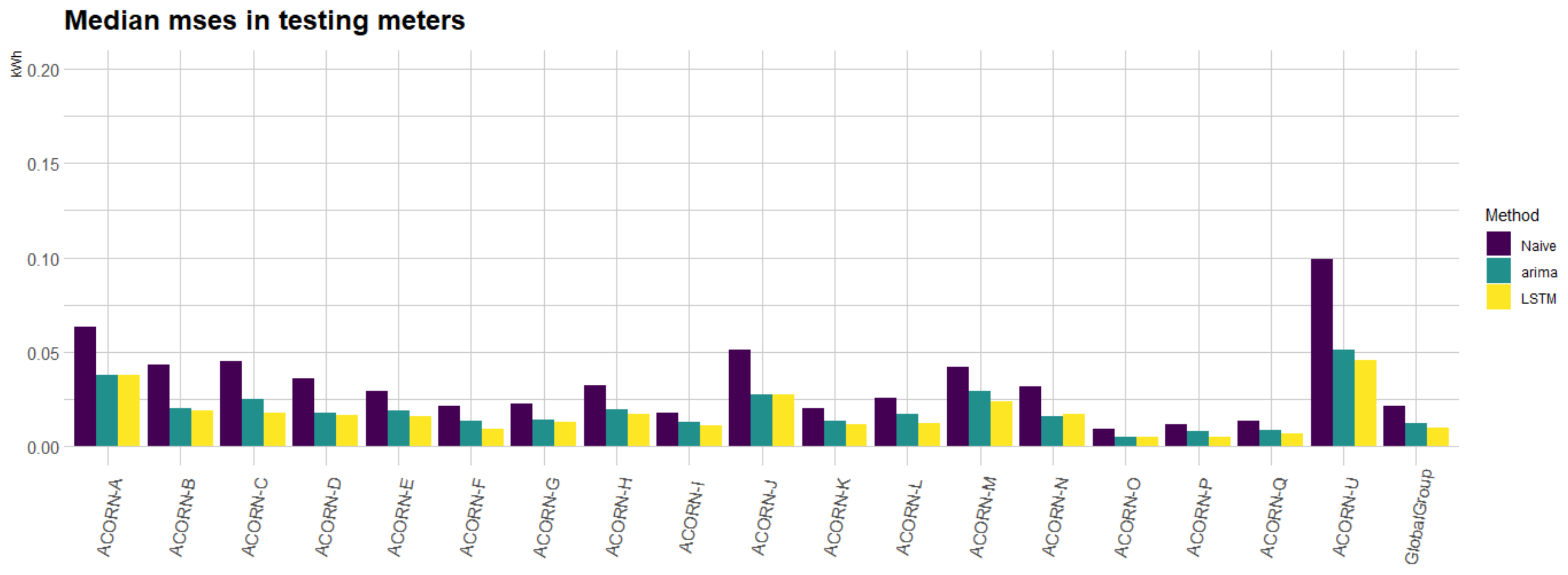
auto.arima, and the proposed LSTM model) for each of the 19 groups considered. In
Figure 13, we can observe the median MSEs for the three implemented approaches along the testing meters. In particular, for each of the smart meters in the testing set for each group, we have computed the median error for all the MSEs obtained in the out-of-sample days in the back-testing. It can be noted how the
auto.arima approach is on average a 5% better than the
naive approach but sometimes is a bit worse. On the other hand, the LSTM approach attains the best performance. In particular, the performance of the LSTM approach is around 19% better than that of the
auto.arima and around 24% better than that of the
naive approach. That implies a good performance of the proposed methodology even for new customers in the database.
On the other hand,
Figure 14 shows the median MSEs for all smart meters along the out-of-sample days. Note the errors of
auto.arima and
naive approaches behave similarly along time (
auto.arima performs around 3% than the
naive), while the proposed LSTM outperforms the
naive approach by 24% on average and the
auto.arima one by 21% on average over
all the out-of-sample periods.
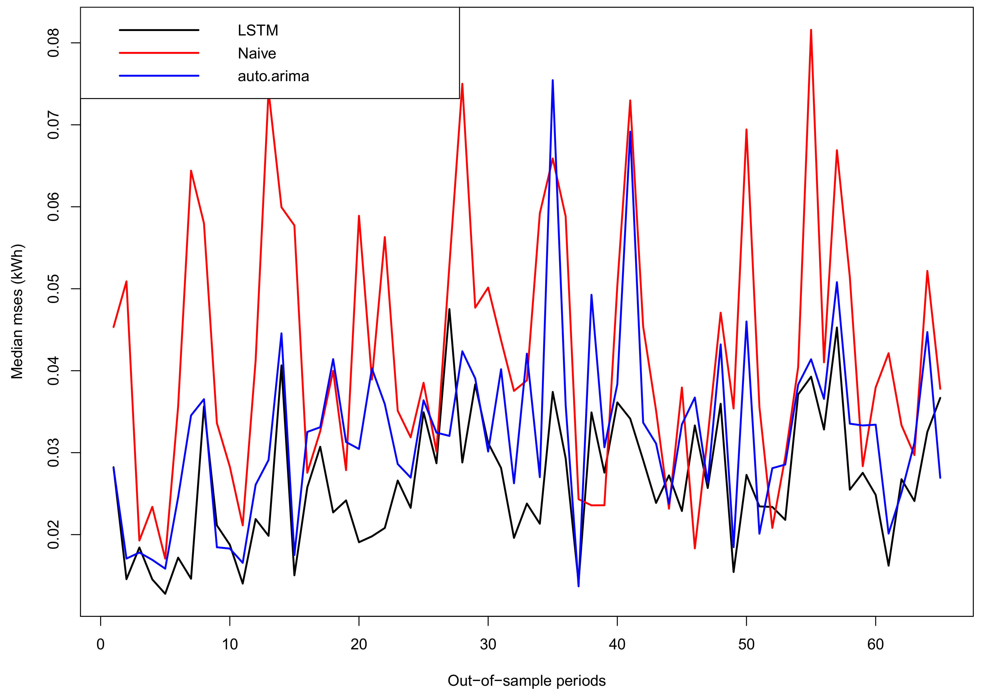
To have a better idea about the forecasted load profiles by the three considered methods, we have selected the ACORN-U group because it has the largest error in
Figure 13. In particular,
Figure 15 shows the evolution of the median MSEs along the 65 out-of-sample days for all the meters in the ACORN-U group. Please note that although forecasting performance depends on time, the proposed LSTM procedure has consistently better out-of-sample errors than the benchmarks.
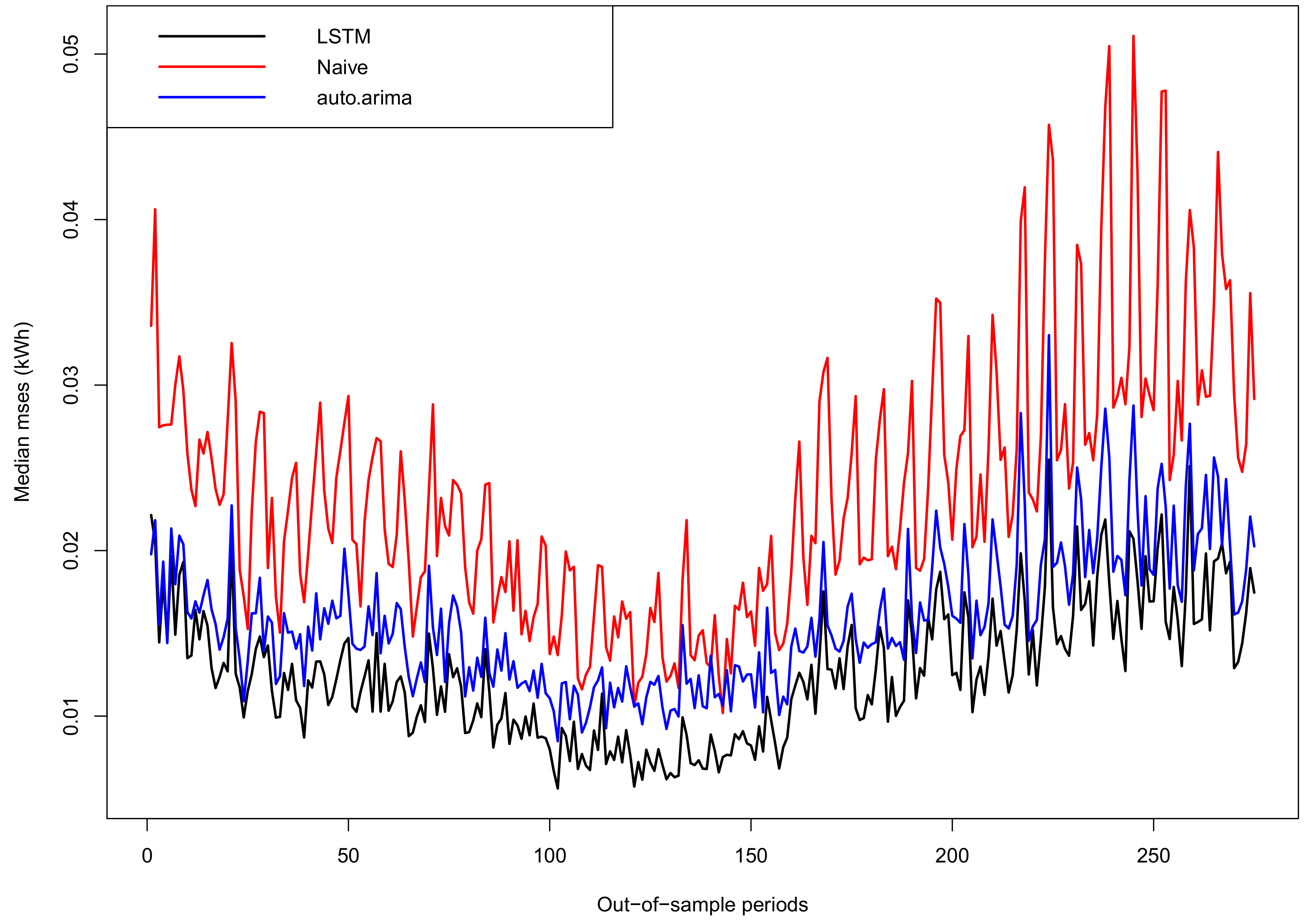
Finally, it is worth analyzing the behavior of our proposal for the Global Group. This group contains 200 time series selected by chance from the other 18 groups. We have chosen 160 of those series to train the unique LSTM and used it to forecast the other 40 series in the testing set.
Figure 16 shows the evolution of the median MSEs along the 275 days in the out-of-sample period for those 40 meters. Again, our method outperforms consistently the two benchmarks by more than 20%, implying the effectiveness of the proposal even when a classification of groups is not available a priori. Of course, if a previous classification of the time series into homogeneous groups is available, our methodology can exploit better this classification to forecast better each group.
The evaluation of these models indicates our proposal have achieved promising and competitive results for all the geo-demographic groups considered in our dataset, implying a good potential for its implementation in large-scale smart-meter load forecasting. Similar conclusions were derived when the mean absolute error (MAE) was used, but for the sake of conciseness they are not presented in the paper.
Although it is difficult to undertake a direct comparison, we can state that the forecasting accuracy of the proposed tool is highly competitive with respect to other state-of-the-art approaches. For instance, [
12] provides forecasts for individual household consumptions of a similar size that ours, but further extend the model input with household activity patterns. Their best reported MSE on the testing days is around 0.2, which is above ours. Similarly, [
32] compares four forecasting models with a subset of households from the same London dataset [
33] that we use, but without considering external regressors. The reported root-mean-square error (RMSE) of the best models is around 0.35 (equivalent to MSE ≈ 0.12) which is also above our average error.
4. Conclusions
We have proposed a general methodology, based on recurrent neural networks and specifically a LSTM model, that is able to forecast consumptions from electricity smart meters in an efficient way for a utility. These forecasts could be used in the implementation of demand response policies, to anticipate and prevent systems peaks or congested lines, to adapt load consumption to renewable generation availability, to identify consumption anomalies that may originate from equipment failure or from electricity theft, etc.
Instead of using traditional and univariate approaches for each smart meter, we propose a single but complex LSTM model that captures the main features of individual consumptions and information from different household consumptions. Consequently, the model attains promising results respect to competitive benchmarks, more than 20% better performance on average along all the testing periods and all the testing meters in our back-testing experiment.
We would like to mention some disadvantages of the proposed approach. As any other complex neural network, there are some difficulties in the design of the network. In particular, there is not a clear way to design the network topology about the configuration of the layers and the corresponding units or neurons. In addition, there are many hyper-parameters to be considered, like the number of layers, the number of units, the activation functions, the type of regularization or dropout, optimization parameters, etc. That implies a great effort and time before the network starts working properly. In addition, neural networks in general are difficult to understand and interpret.
Moreover, the competitive good results depend on the degree of homogeneity of the considered smart meters. In this work, we have used 19 groups of households, the smallest one with 18 smart meters and the biggest one 1001 ones. We have obtained promising results for the near 4000 smart meters, even when the groups have some degree of heterogeneity. However, we do not expect good results for smart meters with very unusual profiles (outliers) in its group. On the other hand, the success of the proposed model is partially explained by the large amount of data used to train the model. Because we are jointly treating and combining the information of all the available time series in a group, the network is able to capture non-linear relations, seasonalities and other hidden patterns that other traditional approaches cannot capture because lack of enough data.
As a summary, our methodology can outperform competitive univariate forecasting tools for electricity consumption, providing an implementable and scalable approach for massive time series forecasting. In particular, it may provide near real-time forecast for hundreds of thousands of smart meters. The model training would need to be done only once every few months, and by using just a representative subset of the smart meters time series. Once the network is trained, and its input properly defined, it can provide short-term smart meters’ forecast at almost no computational costs.
There are several interesting lines of future research to extend and improve the proposed forecasting tool. First, to further increase the forecasting horizon up to one-week ahead (168 h). Second, to try other architectures for the LSTM network and optimize their configuration. Third, to try other datasets (different countries, meteorology, consumption patterns, etc.) and to explore if the proposed architecture is still valid. Finally, to assess the level of uncertainty of each household consumption, to incorporate probabilistic forecasts, in the form of prediction intervals.


